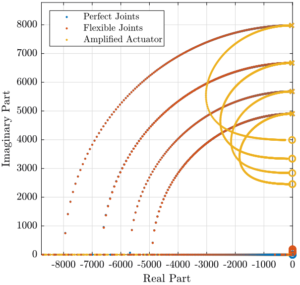
47 KiB
47 KiB
Glossary and Acronyms - Tables
| label | name | description |
|---|---|---|
| ka | \ensuremath{k_a} | Actuator Stiffness in |
| phi | \ensuremath{ɸ} | A woody bush |
| key | abbreviation | full form |
|---|---|---|
| mimo | MIMO | Multiple-Inputs Multiple-Outputs |
| siso | SISO | Single-Input Single-Output |
| nass | NASS | Nano Active Stabilization System |
| lti | LTI | Linear Time Invariant |
| esrf | ESRF | European Synchrotron Radiation Facility |
Title Page
Abstract
\gls{phi}
Résumé
Acknowledgments
Table of Contents
Introduction
Context of this thesis / Background and Motivation
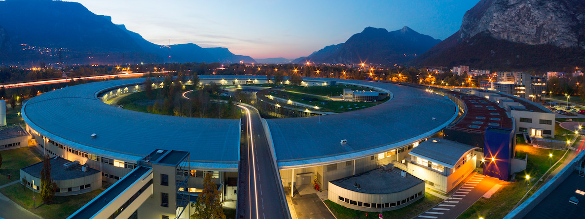
- \gls{esrf} (Figure fig:esrf_picture)
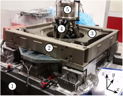
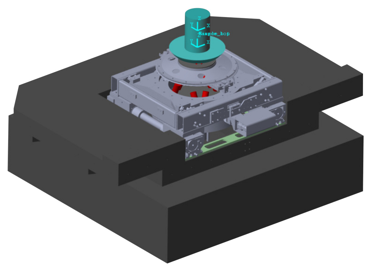
- ID31 and Micro Station (Figure fig:id31_microstation_picture)
\begin{tikzpicture}
  \node[inner sep=0pt, anchor=south west] (photo) at (0,0)
  {\includegraphics[width=0.39\textwidth]{/home/thomas/Cloud/documents/reports/phd-thesis/figs/exp_setup_photo.png}};

  \coordinate[] (aheight) at (photo.north west);
  \coordinate[] (awidth)  at (photo.south east);

  \coordinate[] (granite) at ($0.1*(aheight)+0.1*(awidth)$);
  \coordinate[] (trans)   at ($0.5*(aheight)+0.4*(awidth)$);
  \coordinate[] (tilt)    at ($0.65*(aheight)+0.75*(awidth)$);
  \coordinate[] (hexapod) at ($0.7*(aheight)+0.5*(awidth)$);
  \coordinate[] (sample)  at ($0.9*(aheight)+0.55*(awidth)$);

  % Granite
  \node[labelc] at (granite) {1};
  % Translation stage
  \node[labelc] at (trans) {2};
  % Tilt Stage
  \node[labelc] at (tilt) {3};
  % Micro-Hexapod
  \node[labelc] at (hexapod) {4};
  % Sample
  \node[labelc] at (sample) {5};

  % Axis
  \begin{scope}[shift={($0.07*(aheight)+0.87*(awidth)$)}]
    \draw[->] (0, 0) -- ++(55:0.7) node[above] {$y$};
    \draw[->] (0, 0) -- ++(90:0.9) node[left] {$z$};
    \draw[->] (0, 0) -- ++(-20:0.7) node[above] {$x$};
  \end{scope}
\end{tikzpicture}
Alternative: id31_microstation_cad_view.png (CAD view)
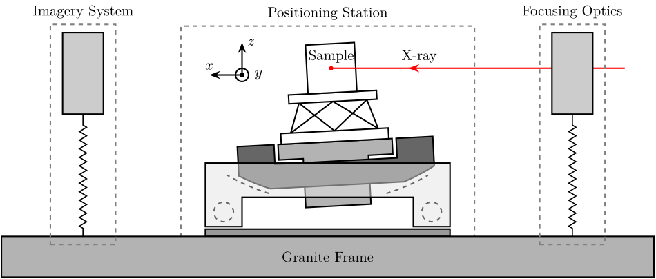
- X-ray beam + detectors + sample stage (Figure fig:id31_beamline_schematic)
  \begin{tikzpicture}
    % Parameters
    \def\blockw{6.0cm}
    \def\blockh{1.2cm}

    \def\tiltdeg{3}
    \coordinate[] (rotationpoint) at (0, 4.5*\blockh);

    \begin{scope}[rotate around={\tiltdeg:(rotationpoint)}]
      % Tilt
      \path[] ([shift=(-120:4*\blockh)]rotationpoint) coordinate(beginarc) arc (-120:-110:4*\blockh) %
      -- ([shift=(-70:4*\blockh)]rotationpoint) arc (-70:-60:4*\blockh)%
      |- ++(-0.15*\blockw, 0.6*\blockh) coordinate (spindlene)%
      |- ($(beginarc) + (0.15*\blockw, 0.2*\blockh)$) coordinate (spindlesw) -- ++(0, 0.4*\blockh) coordinate(tiltte) -| cycle;

      % Spindle
      \coordinate[] (spindlese) at (spindlesw-|spindlene);
      \draw[fill=black!30] ($(spindlese)+(-0.1,0.1)+(-0.1*\blockw, 0)$) -| ($(spindlene)+(-0.1, 0)$) -| coordinate[pos=0.25](spindletop) ($(spindlesw)+(0.1,0.1)$) -| ++(0.1*\blockw, -\blockh) -| coordinate[pos=0.25](spindlebot) cycle;

      % \draw[dashed, color=black!60] ($(spindletop)+(0, 0.2)$) -- ($(spindlebot)+(0,-0.2)$);

      % Tilt
      \draw[fill=black!60] ([shift=(-120:4*\blockh)]rotationpoint) coordinate(beginarc) arc (-120:-110:4*\blockh) %
      -- ([shift=(-70:4*\blockh)]rotationpoint) arc (-70:-60:4*\blockh)%
      |- coordinate (tiltne) ++(-0.15*\blockw, 0.6*\blockh) coordinate (spindlene)%
      |- ($(beginarc) + (0.15*\blockw, 0.2*\blockh)$) coordinate (spindlesw) -- ++(0, 0.4*\blockh) -| cycle;

      % Micro-Hexapod
      \begin{scope}[shift={(spindletop)}]
        % Parameters definitions
        \def\baseh{0.22*\blockh} % Height of the base
        \def\naceh{0.18*\blockh} % Height of the nacelle
        \def\baser{0.22*\blockw} % Radius of the base
        \def\nacer{0.18*\blockw} % Radius of the nacelle

        \def\armr{0.2*\blockh} % Radius of the arms
        \def\basearmborder{0.2}
        \def\nacearmborder{0.2}

        \def\xnace{0} \def\ynace{\blockh-\naceh} \def\anace{0}
        \def\xbase{0} \def\ybase{0} \def\abase{0}

        % Hexapod1
        \begin{scope}[shift={(\xbase, \ybase)}, rotate=\abase]
          % Base
          \draw[fill=white] (-\baser, 0) coordinate[](uhexabot) rectangle (\baser, \baseh);

          \coordinate[] (armbasel) at (-\baser+\basearmborder+\armr, \baseh);
          \coordinate[] (armbasec) at (0, \baseh);
          \coordinate[] (armbaser) at (\baser-\basearmborder-\armr, \baseh);

          \begin{scope}[shift={(\xnace, \ynace)}, rotate=\anace]
            \draw[fill=white] (-\nacer, 0) rectangle (\nacer, \naceh);
            \coordinate[] (uhexatop) at (0, \naceh);
            \coordinate[] (armnacel) at (-\nacer+\nacearmborder+\armr, 0);
            \coordinate[] (armnacec) at (0, 0);
            \coordinate[] (armnacer) at (\nacer-\nacearmborder-\armr, 0);
          \end{scope}

          \draw[] (armbasec) -- (armnacer);
          \draw[] (armbasec) -- (armnacel);
          \draw[] (armbasel) -- coordinate(mhexaw) (armnacel);
          \draw[] (armbasel) -- (armnacec);
          \draw[] (armbaser) -- (armnacec);
          \draw[] (armbaser) -- coordinate(mhexae) (armnacer);
        \end{scope}
      \end{scope}

      % Sample
      \begin{scope}[shift={(uhexatop)}]
        \draw[fill=white] (-0.1*\blockw, 0) coordinate[](samplebot) rectangle coordinate[pos=0.5](samplecenter) node[pos=0.5, above]{Sample} (0.1*\blockw, \blockh) coordinate[](samplene);
        \coordinate[](samplenw) at (-0.1*\blockw, \blockh);
      \end{scope}
    \end{scope}

    \begin{scope}[shift={(0, -0.3*\blockh)}]
      % Translation Stage - fixed part
      \draw[fill=black!40] (-0.5*\blockw, 0) coordinate[](tyb) rectangle (0.5*\blockw, 0.15*\blockh);
      \coordinate[] (measposbot) at (0.5*\blockw, 0);

      % Translation Stage - mobile part
      \draw[fill=black!10, fill opacity=0.5] (-0.5*\blockw, 0.2*\blockh) -- (-0.5*\blockw, 1.5*\blockh) coordinate[](tyt) -- (0.5*\blockw, 1.5*\blockh) -- (0.5*\blockw, 0.2*\blockh) -- (0.35*\blockw, 0.2*\blockh) -- (0.35*\blockw, 0.8*\blockh) -- (-0.35*\blockw, 0.8*\blockh) -- (-0.35*\blockw, 0.2*\blockh) -- cycle;

      % Translation Guidance
      \draw[dashed, color=black!60] ($(-0.5*\blockw, 0)+( 0.075*\blockw,0.5*\blockh)$) circle (0.2*\blockh);
      \draw[dashed, color=black!60] ($( 0.5*\blockw, 0)+(-0.075*\blockw,0.5*\blockh)$) circle (0.2*\blockh);

      % Tilt Guidance
      \draw[dashed, color=black!60] ([shift=(-107:4.1*\blockh)]rotationpoint) arc (-107:-120:4.1*\blockh);
      \draw[dashed, color=black!60] ([shift=( -73:4.1*\blockh)]rotationpoint) arc (-73:-60:4.1*\blockh);
    \end{scope}

    % % Vertical line
    % \draw[dashed, color=black] (samplecenter) -- ++(0, -4*\blockh);
    % \begin{scope}[rotate around={\tiltdeg:(samplecenter)}]
    %   \draw[dashed, color=black] (samplecenter) -- ++(0, -4*\blockh);
    %   \node[] at ($(samplecenter)+(0, -2.3*\blockh)$) {\AxisRotator[rotate=-90]};
    %   \node[right, shift={(0.3,0)}] at ($(samplecenter)+(0, -2.3*\blockh)$) {$\theta_z$};
    % \end{scope}
    % \draw[->] ([shift=(-90:3.6*\blockh)]samplecenter) arc (-90:-87:3.6*\blockh) node[right]{$\theta_y$};

    % Laser
    \begin{scope}[shift={(samplecenter)}]
      \draw[color=red, -<-=0.3] (samplecenter) node[circle, fill=red, inner sep=0pt, minimum size=3pt]{} -- node[pos=0.3, above, color=black]{X-ray} ($(samplecenter)+(1.2*\blockw,0)$);
    \end{scope}

    % Axis
    \begin{scope}[shift={(-0.35*\blockw, 3*\blockh)}]
      \def\axissize{0.8cm}
      \draw[->] (0, 0) -- ++(0, \axissize) node[right]{$z$};
      \draw[->] (0, 0) -- ++(-\axissize, 0) node[above]{$x$};
      \draw[fill, color=black] (0, 0) circle (0.05*\axissize);
      \node[draw, circle, inner sep=0pt, minimum size=0.4*\axissize, label=right:$y$] (yaxis) at (0, 0){};
      % \node[draw, circle, inner sep=0pt, cross, minimum size=0.4*\axissize, label=left:$y$] (yaxis) at (0, 0){};
    \end{scope}

    \node[fit={($(-0.6*\blockw, -0.5*\blockh)$) ($(0.6*\blockw, 4*\blockh)$)}, inner sep=0pt, draw, dashed, color=gray, label={Positioning Station}] (possystem) {};

    \draw[fill=black!30] ($(tyb)+(-5, -1)$) coordinate[](granitesw) rectangle node[pos=0.5]{Granite Frame} ($(measposbot)+(5, 0)$) coordinate[](granitene);

    % Focusing Optics
    \draw[fill=black!20] ($(granitene)+(-1.5, 3)$) rectangle ++(-1, 2);
    \draw[spring] ($(granitene)+(-2, 0)$) -- ++(0, 3);

    \node[fit={($(granitene)+(-2.8, -0.2)$) ($(granitene)+(-1.2, 5.2)$)}, inner sep=0pt, draw, dashed, color=gray, label={Focusing Optics}] () {};

    % Measurement Optics
    \draw[fill=black!20] ($(granitesw)+(1.5, 4)$) rectangle ++(1, 2);
    \draw[spring] ($(granitesw)+(2, 1)$) -- ++(0, 3);

    \node[fit={($(granitesw)+(2.8, 0.8)$) ($(granitesw)+(1.2, 6.2)$)}, inner sep=0pt, draw, dashed, color=gray, label={Imagery System}] () {};
\end{tikzpicture}- Few words about science made on ID31 and why nano-meter accuracy is required
- Typical experiments (tomography, …), various samples (up to 50kg)
- Where to explain the goal of each stage? (e.g. micro-hexapod: static positioning, Ty and Rz: scans, …)
- Example of picture obtained (Figure fig:id31_tomography_result)
- Explain wanted positioning accuracy and why micro-station cannot have this accuracy (backlash, play, thermal expansion, …)
- Speak about the metrology concept, and why it is not included in this thesis
Challenge definition
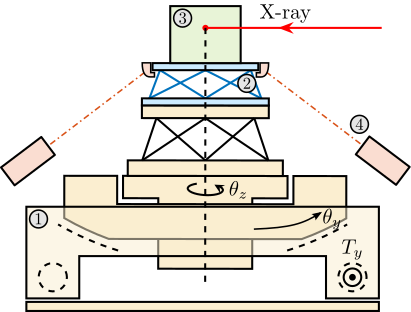
- 6DoF vibration control platform on top of a complex positioning platform
- Goal: Improve accuracy of 6DoF long stroke position platform
- Approach: Mechatronic approach / model based / predictive
- Control: Robust control approach / various payloads. First hexapod with control bandwidth higher than the suspension modes that accepts various payloads?
- Rotation aspect
- Compactness? (more related to mechanical design)
Literature Review
- Hexapods cite:li01_simul_fault_vibrat_isolat_point cite:bishop02_devel_precis_point_contr_vibrat cite:hanieh03_activ_stewar cite:afzali-far16_vibrat_dynam_isotr_hexap_analy_studies cite:naves20_desig ~/Cloud/work-projects/ID31-NASS/matlab/stewart-simscape/org/bibliography.org
- Positioning stations
- Mechatronic approach? cite:rankers98_machin cite:monkhorst04_dynam_error_budget cite:jabben07_mechat
Outline of thesis / Thesis Summary / Thesis Contributions
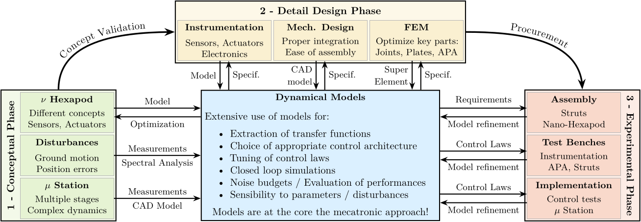
Mechatronic Design Approach / Model Based Design:
- cite:&monkhorst04_dynam_error_budget high costs of the design process: the designed system must be first time right. When the system is finally build, its performance level should satisfy the specifications. No significant changes are allowed in the post design phase. Because of this, the designer wants to be able to predict the performance of the system a-priori and gain insight in the performance limiting factors of the system.
% \graphicspath{ {/home/thomas/Cloud/thesis/papers/dehaeze21_mechatronics_approach_nass/tikz/figs-tikz} }

\begin{tikzpicture}
  % Styles
  \tikzset{myblock/.style= {draw, thin, color=white!70!black, fill=white, text width=3cm, align=center, minimum height=1.4cm}};
  \tikzset{mylabel/.style= {anchor=north, below, font=\bfseries\small, color=black, text width=3cm, align=center}};
  \tikzset{mymodel/.style= {anchor=south, above, font=\small, color=black, text width=3cm, align=center}};
  \tikzset{mystep/.style=  {->, ultra thick}};

  % Blocks
  \node[draw, fill=lightblue, align=center, label={[mylabel, text width=8.0cm] Dynamical Models}, minimum height = 4.5cm, text width = 8.0cm] (model) at (0, 0) {};

  \node[myblock, fill=lightgreen, label={[mylabel] Disturbances},  left = 3 of model.west]                          (dist) {};
  \node[myblock, fill=lightgreen, label={[mylabel] $\mu$ Station}, below = 2pt of dist] (mustation) {};
  \node[myblock, fill=lightgreen, label={[mylabel] $\nu$ Hexapod}, above = 2pt of dist] (nanohexapod) {};

  \node[myblock, fill=lightyellow, label={[mylabel] Mech. Design},    above = 1 of model.north] (mechanical) {};
  \node[myblock, fill=lightyellow, label={[mylabel] Instrumentation}, left  = 2pt of mechanical]  (instrumentation) {};
  \node[myblock, fill=lightyellow, label={[mylabel] FEM},             right = 2pt of mechanical]  (fem) {};

  \node[myblock, fill=lightred, label={[mylabel] Test Benches},   right = 3 of model.east]                          (testbenches) {};
  \node[myblock, fill=lightred, label={[mylabel] Assembly},       above = 2pt of testbenches] (mounting) {};
  \node[myblock, fill=lightred, label={[mylabel] Implementation}, below = 2pt of testbenches] (implementation) {};

  % Text
  \node[anchor=south, above, text width=8cm, align=left] at (model.south) {Extensive use of models for:\begin{itemize}[noitemsep,topsep=5pt]\item Extraction of transfer functions \\ \item Choice of appropriate control architecture \\ \item Tuning of control laws \\ \item Closed loop simulations \\ \item Noise budgets / Evaluation of performances \\ \item Sensibility to parameters / disturbances\end{itemize}\centerline{Models are at the core the mecatronic approach!}};

  \node[mymodel] at (mustation.south)       {Multiple stages     \\ Complex dynamics};
  \node[mymodel] at (dist.south)            {Ground motion       \\ Position errors};
  \node[mymodel] at (nanohexapod.south)     {Different concepts  \\ Sensors, Actuators};

  \node[mymodel] at (instrumentation.south) {Sensors, Actuators  \\ Electronics};
  \node[mymodel] at (mechanical.south)      {Proper integration  \\ Ease of assembly};
  \node[mymodel] at (fem.south)             {Optimize key parts: \\ Joints, Plates, APA};

  \node[mymodel] at (mounting.south)        {Struts              \\ Nano-Hexapod};
  \node[mymodel] at (testbenches.south)     {Instrumentation     \\ APA, Struts};
  \node[mymodel] at (implementation.south)  {Control tests       \\ $\mu$ Station};

  % Links
  \draw[->] (dist.east)      -- node[above, midway]{{\small Measurements}} node[below,midway]{{\small Spectral Analysis}} (dist.east-|model.west);
  \draw[->] (mustation.east) -- node[above, midway]{{\small Measurements}} node[below, midway]{{\small CAD Model}} (mustation.east-|model.west);

  \draw[->] ($(nanohexapod.east-|model.west)-(0, 0.15)$) -- node[below, midway]{{\small Optimization}} ($(nanohexapod.east)-(0, 0.15)$);
  \draw[<-] ($(nanohexapod.east-|model.west)+(0, 0.15)$) -- node[above, midway]{{\small Model}} ($(nanohexapod.east)+(0, 0.15)$);

  \draw[->] ($(fem.south|-model.north)+(0.15, 0)$) -- node[right, midway]{{\small Specif.}} ($(fem.south)+(0.15,0)$);
  \draw[<-] ($(fem.south|-model.north)-(0.15, 0)$) -- node[left, midway,align=right]{{\small Super}\\{\small Element}}  ($(fem.south)-(0.15,0)$);

  \draw[->] ($(mechanical.south|-model.north)+(0.15, 0)$) -- node[right, midway]{{\small Specif.}} ($(mechanical.south)+(0.15,0)$);
  \draw[<-] ($(mechanical.south|-model.north)-(0.15, 0)$) -- node[left, midway,align=right]{{\small CAD}\\{\small model}}        ($(mechanical.south)-(0.15,0)$);

  \draw[->] ($(instrumentation.south|-model.north)+(0.15, 0)$) -- node[right, midway]{{\small Specif.}} ($(instrumentation.south)+(0.15,0)$);
  \draw[<-] ($(instrumentation.south|-model.north)-(0.15, 0)$) -- node[left, midway]{{\small Model}}         ($(instrumentation.south)-(0.15,0)$);

  \draw[->] ($(mounting.west-|model.east)+(0, 0.15)$) -- node[above, midway]{{\small Requirements}} ($(mounting.west)+(0, 0.15)$);
  \draw[<-] ($(mounting.west-|model.east)-(0, 0.15)$) -- node[below, midway]{{\small Model refinement}}   ($(mounting.west)-(0, 0.15)$);

  \draw[->] ($(testbenches.west-|model.east)+(0, 0.15)$) -- node[above, midway]{{\small Control Laws}} ($(testbenches.west)+(0, 0.15)$);
  \draw[<-] ($(testbenches.west-|model.east)-(0, 0.15)$) -- node[below, midway]{{\small Model refinement}}   ($(testbenches.west)-(0, 0.15)$);

  \draw[->] ($(implementation.west-|model.east)+(0, 0.15)$) -- node[above, midway]{{\small Control Laws}} ($(implementation.west)+(0, 0.15)$);
  \draw[<-] ($(implementation.west-|model.east)-(0, 0.15)$) -- node[below, midway]{{\small Model refinement}}   ($(implementation.west)-(0, 0.15)$);

  % Main steps
  \node[font=\bfseries, rotate=90, anchor=south, above] (conceptual_phase_node) at (dist.west) {1 - Conceptual Phase};
  \node[font=\bfseries, above] (detailed_phase_node) at (mechanical.north) {2 - Detail Design Phase};
  \node[font=\bfseries, rotate=-90, anchor=south, above] (implementation_phase_node) at (testbenches.east) {3 - Experimental Phase};
    \begin{scope}[on background layer]
      \node[fit={(conceptual_phase_node.north|-nanohexapod.north) (mustation.south east)}, fill=lightgreen!50!white, draw, inner sep=2pt] (conceptual_phase) {};
      \node[fit={(detailed_phase_node.north-|instrumentation.west) (fem.south east)}, fill=lightyellow!50!white, draw, inner sep=2pt] (detailed_phase) {};
      \node[fit={(implementation_phase_node.north|-mounting.north) (implementation.south west)}, fill=lightred!50!white, draw, inner sep=2pt] (implementation_phase) {};
      % \node[above left] at (dob.south east) {DOB};
    \end{scope}

  % Between main steps
  \draw[mystep, postaction={decorate,decoration={raise=1ex,text along path,text align=center,text={Concept Validation}}}] (conceptual_phase.north) to[out=90, in=180] (detailed_phase.west);
  \draw[mystep, postaction={decorate,decoration={raise=1ex,text along path,text align=center,text={Procurement}}}] (detailed_phase.east) to[out=0, in=90] (implementation_phase.north);

  % % Inside Model
  % \node[inner sep=1pt, outer sep=6pt, anchor=north west, draw, fill=white, thin] (multibodymodel) at ($(model.north west) - (0, 0.5)$)
  %   {\includegraphics[width=5.6cm]{simscape_nano_hexapod.png}};

  % \node[inner sep=1pt, outer sep=6pt, anchor=south west, draw, fill=white, thin] (simscape) at (model.south west)
  %   {\includegraphics[width=5.6cm]{simscape_picture.jpg}};

  % % Feedback Model
  % \node[inner sep=3pt, outer sep=6pt, anchor=north east, draw, fill=white, thin] (simscape_sim) at ($(model.north east) - (0, 0.5)$)
  %   {\includegraphics[width=3.6cm]{simscape_simulations.pdf}};

  % % FeedBack
  % \node[inner sep=3pt, outer sep=6pt, anchor=south east, draw, fill=white, thin] (feedback) at (model.south east)
  %   {\includegraphics[width=3.6cm]{classical_feedback_small.pdf}};
\end{tikzpicture}Goals:
- Design \gls{nass} such that it is easy to control (and maintain). Have good performances by design and not by complex control strategies.
Models:
-
Uniaxial Model:
- Effect of limited support compliance
- Effect of change of payload
-
Rotating Model
- Gyroscopic effects
- Multi Body Model
- Finite Element Models
Conceptual Design Development
minitoc
Uni-axial Model
Introduction
- Explain what we want to capture with this model
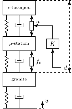
- Schematic of the uniaxial model (with X-ray)
- Identification of disturbances (ground motion, stage vibrations)
- Optimal nano-hexapod stiffness/actuator: Voice coil VS Piezo (conclusion?)
- Control architecture (IFF, DVF, …)?
- Conclusion
\begin{tikzpicture}
  % ====================
  % Parameters
  % ====================
  \def\bracs{0.05} % Brace spacing vertically
  \def\brach{-12pt} % Brace shift horizontaly
  % ====================

  % ====================
  % Ground
  % ====================
  \draw (-0.9, 0) -- (0.9, 0);
  \draw[dashed] (0.9, 0) -- ++(0.5, 0);
  \draw[->] (1.3, 0) -- ++(0, 0.4) node[right]{$w$};
  % ====================

  % ====================
  % Granite
  \begin{scope}[shift={(0, 0)}]
    \draw[fill=white] (-0.9, 1.2) rectangle (0.9, 2.0) node[pos=0.5]{$\scriptstyle\text{granite}$};
    \draw[spring] (-0.7, 0)   -- ++(0, 1.2);
    \draw[damper] ( 0,   0)   -- ++(0, 1.2);

    \draw[dashed] ( 0.9, 2.0) -- ++(2.0, 0) coordinate(xg);

    % \draw[decorate, decoration={brace, amplitude=8pt}, xshift=\brach] %
    % (-0.9, \bracs) -- ++(0, 2.0) node[midway,rotate=90,anchor=south,yshift=10pt]{Granite};
  \end{scope}
  % ====================

  % ====================
  % Stages
  \begin{scope}[shift={(0, 2.0)}]
    \draw[fill=white] (-0.9, 1.2) rectangle (0.9, 2.0) node[pos=0.5]{$\scriptstyle\mu\text{-station}$};

    \coordinate (mustation) at (0.9, 1.6);

    \draw[spring]   (-0.7, 0) -- ++(0, 1.2);
    \draw[damper]   ( 0,   0) -- ++(0, 1.2);
    \draw[actuator] ( 0.7, 0) -- ++(0, 1.2) node[midway, right=0.1](ft){$f_t$};

    % \draw[decorate, decoration={brace, amplitude=8pt}, xshift=\brach] %
    % (-0.9, \bracs) -- ++(0, 2.0) node[midway,rotate=90,anchor=south,yshift=10pt]{$\mu\text{-station}$};
  \end{scope}
  % ====================


  % ====================
  % NASS
  \begin{scope}[shift={(0, 4.0)}]
    \draw[fill=white] (-0.9, 1.2) rectangle (0.9, 2.0) node[pos=0.5]{$\scriptstyle\nu\text{-hexapod}$};
    \draw[dashed] (0.9, 2.0) -- ++(2.0, 0) coordinate(xnpos);

    \draw[spring]   (-0.7, 0) -- ++(0, 1.2) node[midway, left=0.1]{};
    \draw[damper]   ( 0,   0) -- ++(0, 1.2) node[midway, left=0.2]{};
    \draw[actuator] ( 0.7, 0) -- ++(0, 1.2) coordinate[midway, right=0.1](f);

    % \draw[decorate, decoration={brace, amplitude=8pt}, xshift=\brach] %
    % (-0.9, \bracs) -- ++(0, 2.2) node[midway,rotate=90,anchor=south,yshift=10pt]{$\nu\text{-hexapod}$};
  \end{scope}
  % ====================

  % ====================
  % Measured Displacement
  \draw[<->, dashed] ($(xg)+(-0.1, 0)$) node[above left](d){$d$} -- ($(xnpos)+(-0.1, 0)$);
  % ====================

  % ====================
  % IFF Control
  % \node[block={2em}{1.5em}, right=0.6 of fsensn] (iff) {$K_{\scriptscriptstyle IFF}$};
  % \node[addb] (ctrladd) at (f-|iff) {};
  \node[block={2em}{1.5em}, right=0.6 of mustation] (ctrl) {$K$};

  % \draw[->] (fsensn.east)  -- node[midway, above]{$\tau_m$} (iff.west);
  % \draw[->] (iff.south)    -- (ctrladd.north);
  % \draw[->] (ctrladd.west) -- (f.east) node[above right]{$u$};
  \draw[->] (d.west)       -| (ctrl.south);
  \draw[->] (ctrl.north)   |- (f) node[above right]{$u$};
  % ====================
\end{tikzpicture}Micro Station Model
Nano Hexapod Model
Disturbance Identification
Open Loop Dynamic Noise Budgeting
Active Damping
Conclusion: IFF is better for this application
Integral Force Feedback
- Mass spring damper model
- Root Locus
- Sensitivity to disturbances
Direct Velocity Feedback
- Mass spring damper model
- Root Locus
- Sensitivity to disturbances
Position Feedback Controller
Effect of support compliance
- goal: make the nano-hexapod independent of the support compliance
- Simple 2DoF model
- Generalized to any support compliance
- conclusion: frequency of nano-hexapod resonances should be lower than first suspension mode of the support
Effect of payload dynamics
- goal: be robust to a change of payload
- Simple 2DoF model
- Generalized to any payload dynamics
Conclusion
Effect of rotation
Introduction
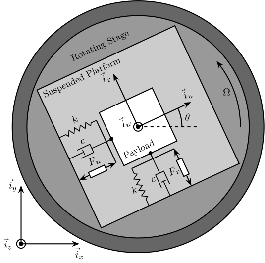
System Description and Analysis
- x-y-Rz model
- explain why this is representing the NASS
- Equation of motion
- Centrifugal forces, Coriolis
  \begin{tikzpicture}
    % Angle
    \def\thetau{25}

    % Rotational Stage
    \draw[fill=black!60!white] (0, 0) circle (4.3);
    \draw[fill=black!40!white] (0, 0) circle (3.8);

    % Label
    \node[anchor=north west, rotate=\thetau] at (-2.5, 2.5) {\small Rotating Stage};

    % Rotating Scope
    \begin{scope}[rotate=\thetau]
      % Rotating Frame
      \draw[fill=black!20!white] (-2.6, -2.6) rectangle (2.6, 2.6);
      % Label
      \node[anchor=north west, rotate=\thetau] at (-2.6, 2.6) {\small Suspended Platform};

      % Mass
      \draw[fill=white] (-1, -1) rectangle (1, 1);
      % Label
      \node[anchor=south west, rotate=\thetau] at (-1, -1) {\small Payload};

      % Attached Points
      \node[] at (-1, 0){$\bullet$};
      \draw[] (-1, 0) -- ++(-0.2, 0) coordinate(cu);
      \draw[] ($(cu) + (0, -0.8)$) coordinate(actu) -- ($(cu) + (0, 0.8)$) coordinate(ku);
      \node[] at (0, -1){$\bullet$};
      \draw[] (0, -1) -- ++(0, -0.2) coordinate(cv);
      \draw[] ($(cv) + (-0.8, 0)$)coordinate(kv) -- ($(cv) + (0.8, 0)$) coordinate(actv);

      % Spring and Actuator for U
      \draw[actuator={0.6}{0.2}] (actu) -- node[above=0.1, rotate=\thetau]{$F_u$} (actu-|-2.6,0);
      \draw[spring=0.2] (ku) -- node[above=0.1, rotate=\thetau]{$k$} (ku-|-2.6,0);
      \draw[damper={8}{8}] (cu) -- node[above left=0.2 and -0.1, rotate=\thetau]{$c$} (cu-|-2.6,0);

      \draw[actuator={0.6}{0.2}] (actv) -- node[left, rotate=\thetau]{$F_v$} (actv|-0,-2.6);
      \draw[spring=0.2] (kv) -- node[left, rotate=\thetau]{$k$} (kv|-0,-2.6);
      \draw[damper={8}{8}] (cv) -- node[left=0.1, rotate=\thetau]{$c$} (cv|-0,-2.6);
    \end{scope}

    % Inertial Frame
    \draw[->] (-4, -4) -- ++(2, 0) node[below]{$\vec{i}_x$};
    \draw[->] (-4, -4) -- ++(0, 2) node[left]{$\vec{i}_y$};
    \draw[fill, color=black] (-4, -4) circle (0.06);
    \node[draw, circle, inner sep=0pt, minimum size=0.3cm, label=left:$\vec{i}_z$] at (-4, -4){};

    \draw[->] (0, 0) node[above left, rotate=\thetau]{$\vec{i}_w$} -- ++(\thetau:2) node[above, rotate=\thetau]{$\vec{i}_u$};
    \draw[->] (0, 0) -- ++(\thetau+90:2) node[left, rotate=\thetau]{$\vec{i}_v$};
    \draw[fill, color=black] (0,0) circle (0.06);
    \node[draw, circle, inner sep=0pt, minimum size=0.3cm] at (0, 0){};
    \draw[dashed] (0, 0) -- ++(2, 0);
    \draw[] (1.5, 0) arc (0:\thetau:1.5) node[midway, right]{$\theta$};

    \draw[->] (3.5, 0) arc (0:40:3.5) node[midway, left]{$\Omega$};
\end{tikzpicture}Integral Force Feedback
- Control diagram
- Root Locus: unstable with pure IFF
IFF with an High Pass Filter
IFF with a stiffness in parallel with the force sensor
Relative Damping Control
Comparison of Active Damping Techniques
Rotating Nano-Hexapod
Nano Active Stabilization System with rotation
Conclusion
- problem with voice coil actuator
- Two solutions: add parallel stiffness, or change controller
- Conclusion: minimum stiffness is required
- APA is a nice architecture for parallel stiffness + integrated force sensor (have to speak about IFF before that)
Micro Station - Modal Analysis
Introduction
Conclusion:
- complex dynamics: need multi-body model of the micro-station to represent the limited compliance…
Measurement Setup
Frequency Analysis
Modal Analysis
Micro Station - Multi Body Model
Kinematics
- Small overview of each stage and associated stiffnesses / inertia
- schematic that shows to considered DoF
- import from CAD
Modal Analysis and Dynamic Modeling
- Picture of the experimental setup
- Location of accelerometers
- Show obtained modes
- Validation of rigid body assumption
- Explain how this helps tuning the multi-body model
Disturbances and Positioning errors
Validation of the Model
- Most important metric: support compliance
- Compare model and measurement
Nano Hexapod - Multi Body Model
Introduction
- What we want to capture with this model
- Explain what is a multi body model (rigid body, springs, etc…)
- Key elements (plates, joints, struts): for now simplistic model (rigid body elements, perfect joints, …), but in next section, FEM will be used
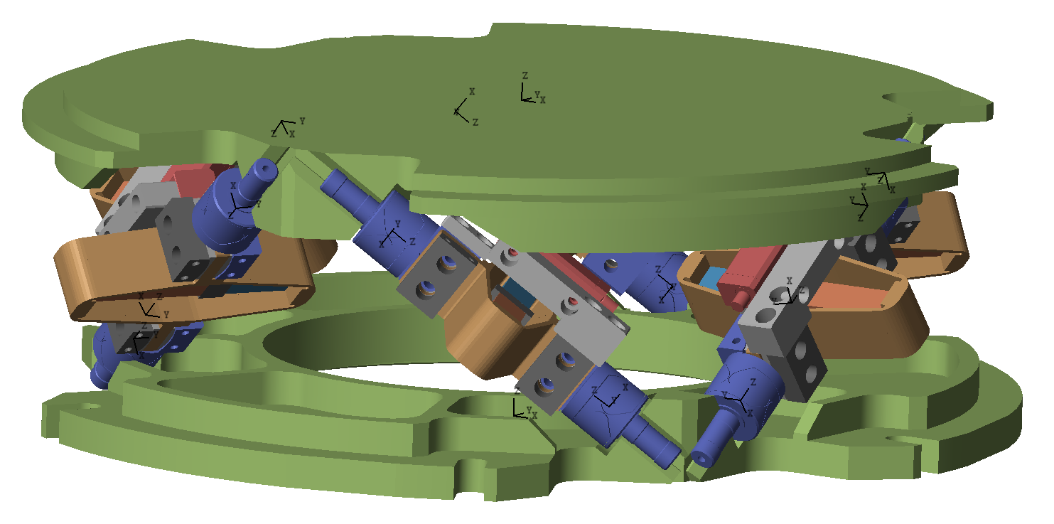
- Matlab/Simulink developed toolbox for the study of Stewart platforms
Stewart Platform Architecture
Configurable Simscape Model: ~/Cloud/work-projects/ID31-NASS/matlab/stewart-simscape/org
- Explain the different frames, etc…
- Little review
-
explain key elements:
- two plates
- joints
- actuators
- explain advantages compared to serial architecture
Kinematics
- Well define elements, frames, …
- Derivation of jacobian matrices: for forces and for displacement
- Explain this is true for small displacements (show how small)
Model of an Amplified Piezoelectric Actuator
- APA test bench
- Piezoelectric effects
- mass spring damper representation (2dof)
- Compare the model and the experiment
- Here, just a basic 2DoF model of the APA is used
Control Architecture - Concept Validation
Introduction
Discussion of:
- Transformation matrices / control architecture (computation of the position error in the frame of the nano-hexapod)
- Control of parallel architectures
- Control in the frame of struts or cartesian?
- Effect of rotation on IFF? => APA
- HAC-LAC
- New noise budgeting?
Control Kinematics
- Explain how the position error can be expressed in the frame of the nano-hexapod
- block diagram
- Explain how to go from external metrology to the frame of the nano-hexapod
High Authority Control - Low Authority Control (HAC-LAC)
- general idea
- case for parallel manipulator: decentralized LAC + centralized HAC
Decoupling Strategies for parallel manipulators
- Jacobian matrices, CoK, CoM, …
- Discussion of cubic architecture
- SVD, Modal, …
Decentralized Integral Force Feedback (LAC)
- Root Locus
- Damping optimization
Decoupled Dynamics
- Centralized HAC
- Control in the frame of the struts
- Effect of IFF
Centralized Position Controller (HAC)
- Decoupled plant
- Controller design
Conceptual Design - Conclusion
Detailed Design
minitoc
Nano-Hexapod Kinematics - Optimal Geometry?
- Maybe this can be just merged with the last section in this chapter?
Introduction
Optimal strut orientation
Cubic Architecture: a Special Case?
Nano-Hexapod Dynamics - Including Flexible elements in the Multi-body model
- Should this be an appendix?
Introduction
Reduced order flexible bodies cite:brumund21_multib_simul_reduc_order_flexib_bodies_fea
- Used with APA, Flexible joints, Plates
Reduced order flexible bodies
- Quick explanation of the theory
- Implementation with Ansys (or Comsol) and Simscape
Numerical Validation
- Numerical Validation Ansys VS Simscape (APA)
- Figure with 0 and 1kg mass
Experimental Validation
- Test bench
- Obtained transfer functions and comparison with Simscape model with reduced order flexible body
Actuator Choice
Introduction
- From previous study: APA seems a nice choice
- First tests with the APA95ML: validation of a basic model (maybe already presented)
- Optimal stiffness?
- Talk about piezoelectric actuator? bandwidth? noise?
- Specifications: stiffness, stroke, … => choice of the APA
- FEM of the APA
- Validation with flexible APA in the simscape model
Model
Experimental System Identification
- Experimental validation (granite test bench)
- Electrical parameters
- Required instrumentation to read force sensor?
- Add resistor to include high pass filtering: no risk of saturating the ADC
- Estimation of piezoelectric parameters
Validation with Simscape model
- Tuned Simscape model
- IFF results: OK
Design of Nano-Hexapod Flexible Joints
Introduction
- Perfect flexible joint
- Imperfection of the flexible joint: Model
- Study of the effect of limited stiffness in constrain directions and non-null stiffness in other directions
- Obtained Specification
- Design optimisation (FEM)
- Implementation of flexible elements in the Simscape model: close to simplified model
Effect of flexible joint characteristics on obtained dynamics
- Based on Simscape model
- Effect of axial stiffness, bending stiffness, …
- Obtained specifications (trade-off)
Flexible joint geometry optimization
- Chosen geometry
- Show different existing geometry for flexible joints used on hexapods
- Optimisation with Ansys
- Validation with Simscape model
Experimental identification
- Experimental validation, characterisation (study)
- Visual inspection
- Test bench
- Obtained results
Choice of Instrumentation
Introduction
-
Discussion of the choice of other elements:
- Encoder
- DAC
- ADC (reading of the force sensors)
- real time controller
- Voltage amplifiers
- Give some requirements + chosen elements + measurements / validation
DAC and ADC
- Force sensor
Voltage amplifier (link)
- Test Bench: capacitive load, ADC, DAC, Instrumentation amplifier
- Noise measurement
- Transfer function measurement
Encoder (link)
- Noise measurement
Obtained Design
- Explain again the different specifications in terms of space, payload, etc..
- CAD view of the nano-hexapod
- Chosen geometry, materials, ease of mounting, cabling, …
- Validation on Simscape with accurate model?
Detailed Design - Conclusion
Experimental Validation
minitoc
Abstract
Amplified Piezoelectric Actuator
Flexible Joints
Struts
SCHEDULED:
Nano-Hexapod
Rotating Nano-Hexapod
ID31 Micro Station
Experimental Validation - Conclusion
Conclusion and Future Work
Alternative Architecture
Appendix
Mathematical Tools for Mechatronics
Feedback Control
Dynamical Noise Budgeting
Power Spectral Density
Cumulative Amplitude Spectrum
Stewart Platform - Kinematics
Bibliography
List of Publications
Glossary
Footnotes
1this is a footnote with citation cite:&dehaeze21_mechat_approac_devel_nano_activ_stabil_system.
