spectral-analysis/index.org

Compute Spectral Densities of signals with Matlab

• Sensitivity of the instrumentation
• Convert the time domain from volts to velocity
• Power Spectral Density and Amplitude Spectral Density
• Modification of a signal's Power Spectral Density when going through an LTI system
• From PSD of the velocity to the PSD of the displacement
• Bibliography

This document presents the mathematics as well as the matlab scripts to do the spectral analysis of a measured signal.

Typically this signal is coming from an inertial sensor, a force sensor or any other sensor.

We here take the example of a signal coming from a Geophone measurement the vertical velocity of the floor at the ESRF.

Sensitivity of the instrumentation

The measured signal $x$ by the ADC is in Volts. The corresponding real velocity $v$ in m/s.

To obtain the real quantity as measured by the sensor, one have to know the sensitivity of the sensors and electronics used.

Schematic of the instrumentation used for the measurement

Convert the time domain from volts to velocity

Let's say, we know that the sensitivity of the geophone used is \[ G_g(s) = G_0 \frac{\frac{s}{2\pi f_0}}{1 + \frac{s}{2\pi f_0}} \quad \left[\frac{V}{m/s}\right] \]

  G0 = 88; % Sensitivity [V/(m/s)]
  f0 = 2; % Cut-off frequency [Hz]

  Gg = G0*(s/2/pi/f0)/(1+s/2/pi/f0);

And the gain of the amplifier is 1000: $G_m(s) = 1000$.

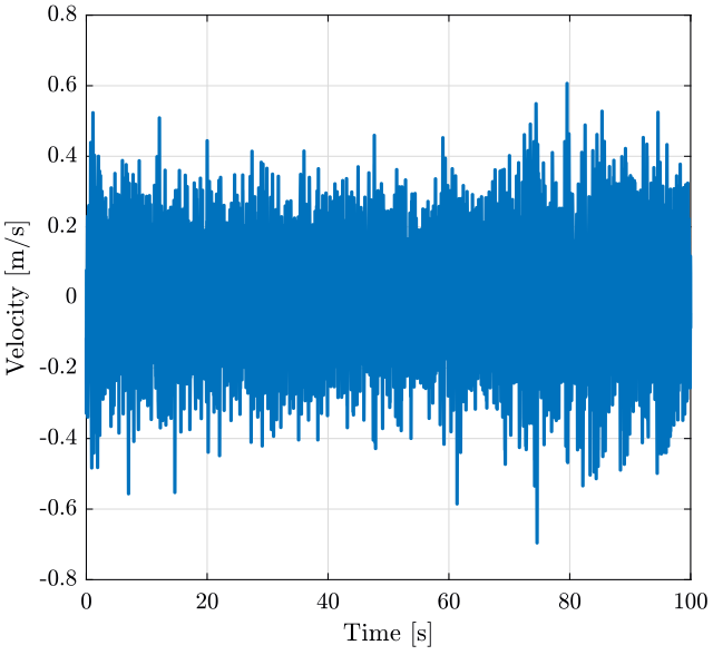
  Gm = 1000;

If ${G_m(s)}^{-1} {G_g(s)}^{-1}$ is proper, we can simulate this dynamical system to go from the voltage to the velocity units (figure fig:voltage_to_velocity).

  data = load('mat/data_028.mat', 'data'); data = data.data;

  t = data(:, 3); % [s]
  x = data(:, 1)-mean(data(:, 1)); % The offset if removed (coming from the voltage amplifier) [v]

  dt = t(2)-t(1); Fs = 1/dt;

Schematic of the instrumentation used for the measurement

We simulate this system with matlab:

  v = lsim(inv(Gg*Gm), v, t);

And we plot the obtained velocity

  figure;
  plot(t, v);
  xlabel("Time [s]"); ylabel("Velocity [m/s]");

  <<plt-matlab>>

Measured Velocity

Power Spectral Density and Amplitude Spectral Density

We now have the velocity in the time domain: \[ v(t)\ [m/s] \]

To compute the Power Spectral Density (PSD): \[ S_v(f)\ \left[\frac{(m/s)^2}{Hz}\right] \]

To compute that with matlab, we use the pwelch function.

We first have to defined a window:

  win = hanning(ceil(10*Fs)); % 10s window

  [Sv, f] = pwelch(v, win, [], [], Fs);

  figure;
  loglog(f, Sv);
  xlabel('Frequency [Hz]');
  ylabel('Power Spectral Density $\left[\frac{(m/s)^2}{Hz}\right]$')

  <<plt-matlab>>

The Amplitude Spectral Density (ASD) is the square root of the Power Spectral Density:

Power Spectral Density of the measured velocity

\begin{equation} \Gamma_{vv}(f) = \sqrt{S_{vv}(f)} \quad \left[ \frac{m/s}{\sqrt{Hz}} \right] \end{equation}

  figure;
  loglog(f, sqrt(Sv));
  xlabel('Frequency [Hz]');
  ylabel('Amplitude Spectral Density $\left[\frac{m/s}{\sqrt{Hz}}\right]$')

  <<plt-matlab>>

Power Spectral Density of the measured velocity

Modification of a signal's Power Spectral Density when going through an LTI system

Schematic of the instrumentation used for the measurement

We can show that:

\begin{equation} S_{yy}(\omega) = \left|G(j\omega)\right|^2 S_{xx}(\omega) \end{equation}

And we also have:

\begin{equation} \Gamma_{yy}(\omega) = \left|G(j\omega)\right| \Gamma_{xx}(\omega) \end{equation}

From PSD of the velocity to the PSD of the displacement

Schematic of the instrumentation used for the measurement

The displacement is the integral of the velocity.

We then have that

\begin{equation} S_{xx}(\omega) = \left|\frac{1}{j \omega}\right|^2 S_{vv}(\omega) \end{equation}

Using a frequency variable in Hz:

\begin{equation} S_{xx}(f) = \left| \frac{1}{j 2\pi f} \right|^2 S_{vv}(f) \end{equation}

For the Amplitude Spectral Density:

\begin{equation} \Gamma_{xx}(f) = \frac{1}{2\pi f} \Gamma_{vv}(f) \end{equation}

\begin{equation} S_{xx}(\omega = 1) = S_{vv}(\omega = 1) \end{equation}

Now if we want to obtain the Power Spectral Density of the Position or Acceleration: For each frequency: \[ \left| \frac{d sin(2 \pi f t)}{dt} \right| = | 2 \pi f | \times | \cos(2\pi f t) | \]

\[ \left| \int_0^t sin(2 \pi f \tau) d\tau \right| = \left| \frac{1}{2 \pi f} \right| \times | \cos(2\pi f t) | \]

\[ ASD_x(f) = \frac{1}{2\pi f} ASD_v(f) \ \left[\frac{m}{\sqrt{Hz}}\right] \]

\[ ASD_a(f) = 2\pi f ASD_v(f) \ \left[\frac{m/s^2}{\sqrt{Hz}}\right] \] And we have \[ PSD_x(f) = {ASD_x(f)}^2 = \frac{1}{(2 \pi f)^2} {ASD_v(f)}^2 = \frac{1}{(2 \pi f)^2} PSD_v(f) \]

Note here that we always have \[ PSD_x \left(f = \frac{1}{2\pi}\right) = PSD_v \left(f = \frac{1}{2\pi}\right) = PSD_a \left(f = \frac{1}{2\pi}\right), \quad \frac{1}{2\pi} \approx 0.16 [Hz] \]

If we want to compute the Cumulative Power Spectrum: \[ CPS_v(f) = \int_0^f PSD_v(\nu) d\nu \quad [(m/s)^2] \]

We can also want to integrate from high frequency to low frequency: \[ CPS_v(f) = \int_f^\infty PSD_v(\nu) d\nu \quad [(m/s)^2] \]

The Cumulative Amplitude Spectrum is then the square root of the Cumulative Power Spectrum: \[ CAS_v(f) = \sqrt{CPS_v(f)} = \sqrt{\int_f^\infty PSD_v(\nu) d\nu} \quad [m/s] \]

Then, we can obtain the Root Mean Square value of the velocity: \[ v_{\text{rms}} = CAS_v(0) \quad [m/s \ \text{rms}] \]

Bibliography   ignore

bibliographystyle:unsrt bibliography:ref.bib