phd-test-bench-struts/test-bench-struts.org

Test Bench - Nano-Hexapod Struts

• Introduction
• Mounting Procedure
  • Introduction
  • Mounting Bench
  • Mounting Procedure
  • Mounted Struts
• Spurious resonances
  • Introduction
  • Measurement Setup
  • Without Encoder
  • With Encoder
  • Conclusion
• Dynamical measurements
  • Introduction
  • Measurement on Strut 1
    • Introduction
    • Without Encoder
      • FRF Identification - Setup
      • FRF Identification - Interferometer
      • FRF Identification - IFF
    • With Encoder
      • Introduction
      • Measurement Data
      • FRF Identification - Interferometer
      • FRF Identification - Encoder
      • APA Resonances Frequency
      • FRF Identification - Force Sensor
      • Non-Minimum phase zero?
  • Comparison of all the Struts
    • Introduction
    • FRF Identification - Setup
    • FRF Identification - Encoder
    • FRF Identification - Interferometer
    • FRF Identification - Force Sensor
    • Misalignment of the APA and flexible joints
    • Conclusion
  • Comparison of all the (re-aligned) Struts
    • Introduction
    • Measured misalignment of the APA and flexible joints
    • FRF Identification - Setup
    • FRF Identification - Encoder
    • FRF Identification - Force Sensor
    • Conclusion
• Simscape Model
  • Introduction
  • Comparison with the 2-DoF Model
    • First Identification
    • Comparison with the experimental Data
  • Comparison with the Flexible Model
    • First Identification
    • Comparison with the experimental Data
  • Effect of a misalignment of the APA and flexible joints on the transfer function from actuator to encoder
    • Introduction
    • Perfectly aligned APA
    • Effect of a misalignment in y
    • Effect of a misalignment in x
    • Find the misalignment of each strut
  • Effect of flexible joint's characteristics
    • Introduction
    • Effect of bending stiffness of the flexible joints
    • Effect of axial stiffness of the flexible joints
    • Effect of bending damping
  • Comparison with identified misalignment
• Conclusion
• Bibliography

---

This report is also available as a pdf.

---

Introduction   ignore

In this document, a test-bench is used to characterize the struts of the nano-hexapod.

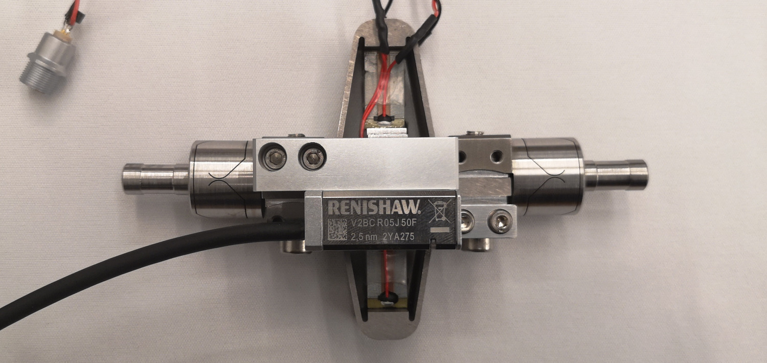
Each strut includes (Figure ref:fig:test_struts_picture_strut):

• 2 flexible joints at each ends. These flexible joints have been characterized in a separate test bench (see …).
• 1 Amplified Piezoelectric Actuator (APA300ML) (described in Section …). Two stacks are used as an actuator and one stack as a (force) sensor.
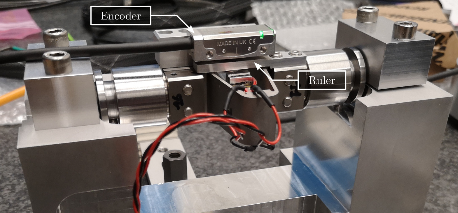
• 1 encoder (Renishaw Vionic) that has been characterized in a separate test bench (see …).

Then the struts are mounted (procedure described in Section ref:sec:test_struts_mounting), and are fixed to the same measurement bench. The goals are to:

• Section ref:sec:test_struts_dynamical_meas: Identify the dynamics from the generated DAC voltage to:

  • the sensors stack generated voltage
  • the measured displacement by the encoder
  • the measured displacement by the interferometer (representing encoders that would be fixed to the nano-hexapod's plates instead of the struts)
• Section ref:sec:test_struts_simscape: Compare the measurements with the Simscape model of the struts and tune the models

The final goal of the work presented in this document is to have an accurate Simscape model of the struts that can then be included in the Simscape model of the nano-hexapod.

Sections	Matlab File
Section ref:sec:test_struts_flexible_modes	test_struts_1_flexible_modes.m
Section ref:sec:test_struts_dynamical_meas	test_struts_2_dynamical_meas.m
Section ref:sec:test_struts_mounting	test_struts_3_simscape_model.m

Mounting Procedure

<<sec:test_struts_mounting>>

Introduction   ignore

Mounting Bench

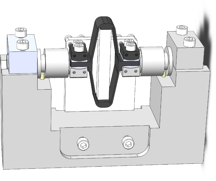
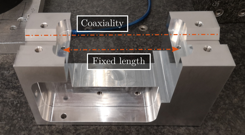
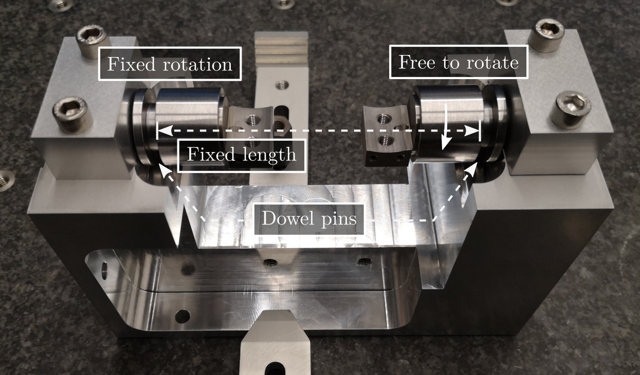
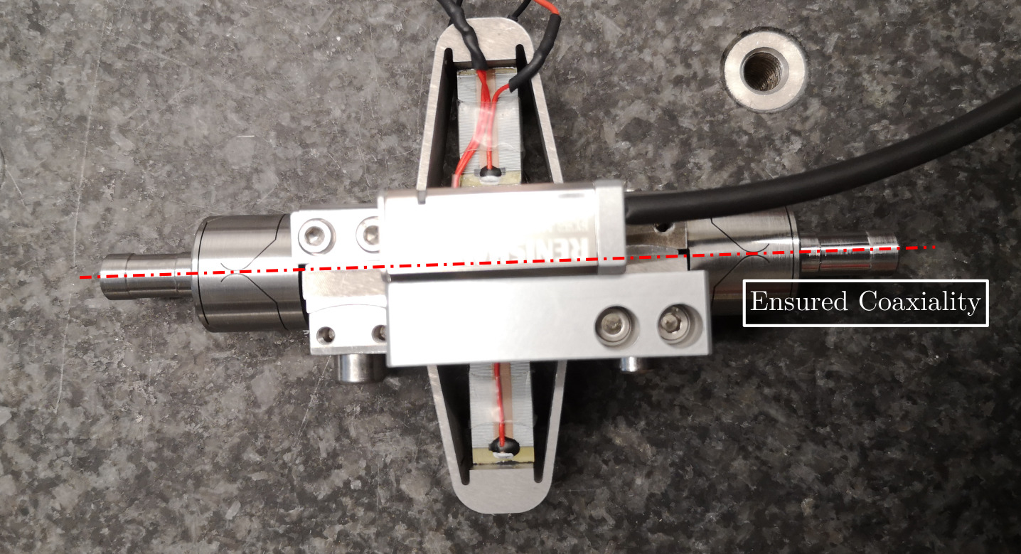
A mounting bench is used to greatly simply the mounting of the struts as well as ensuring the correct strut length and coaxiality of the flexible joint's interfaces. This is very important in order to not loose any stroke when the struts will be mounted on the nano-hexapod.

A CAD view of the mounting bench is shown in Figure ref:fig:test_struts_mounting_bench_first_concept.

The main part of the bench is here to ensure both the correct strut length and strut coaxiality as shown in Figure ref:fig:test_struts_mounting_step_0.

The tight tolerances of this element has been verified as shown in Figure ref:fig:test_struts_mounting_bench_first_concept and were found to comply with the requirements.

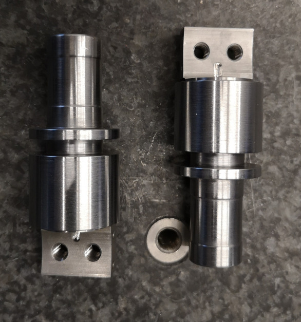
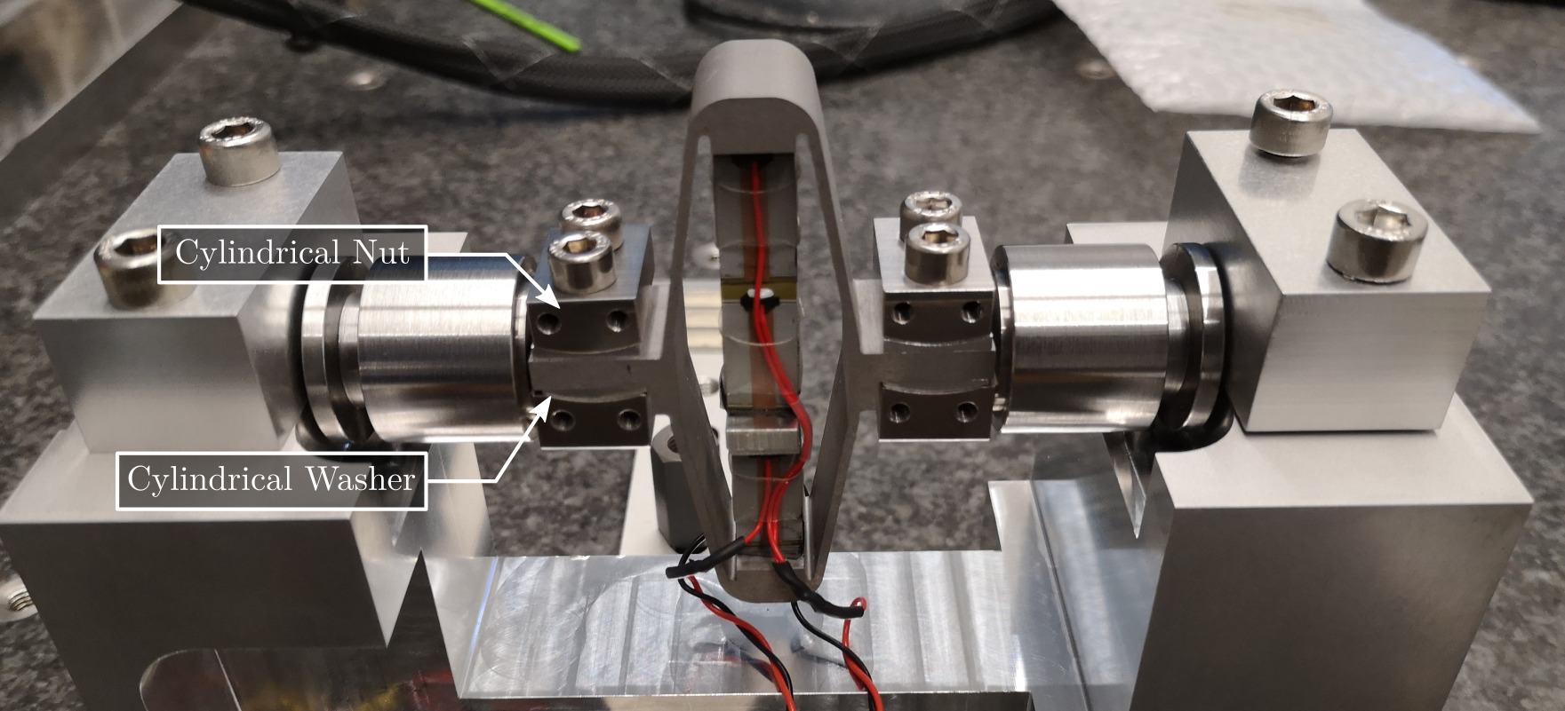
The flexible joints are rigidly fixed to cylindrical tools shown in Figure ref:fig:cylindrical_mounting_part which are then mounted on the mounting tool shown in Figure ref:fig:test_struts_mounting_step_0. This cylindrical tool is here to protect the flexible joints when tightening the screws and therefore applying large torque.

Mounting Procedure

The mounting procedure is as follows:

1. Screw flexible joints inside the cylindrical interface element shown in Figure ref:fig:cylindrical_mounting_part (Figure ref:fig:test_struts_mounting_step_1)
2. Fix the two interface elements. One of the two should be clamped, the other one should have its axial rotation free. Visually align the clamped one horizontally. (Figure ref:fig:test_struts_mounting_step_2)
3. Put cylindrical washers, APA and interface pieces on top of the flexible joints (Figure ref:fig:test_struts_mounting_step_3)
4. Put the 4 screws just in contact such that everything is correctly positioned and such that the "free" flexible joint is correctly oriented
5. Put the 8 lateral screws in contact
6. Tighten the 4 screws to fix the APA on the two flexible joints (using a torque screwdriver)
7. Remove the 4 laterals screws
8. (optional) Put the APA horizontally and fix the encoder and align it to maximize the contrast (Figure ref:fig:test_struts_mounting_step_4)

Mounted Struts

After removing the strut from the mounting bench, we obtain a strut with ensured coaxiality between the two flexible joint's interfaces (Figure ref:fig:test_struts_mounted_strut).

Spurious resonances

<<sec:test_struts_flexible_modes>>

Introduction

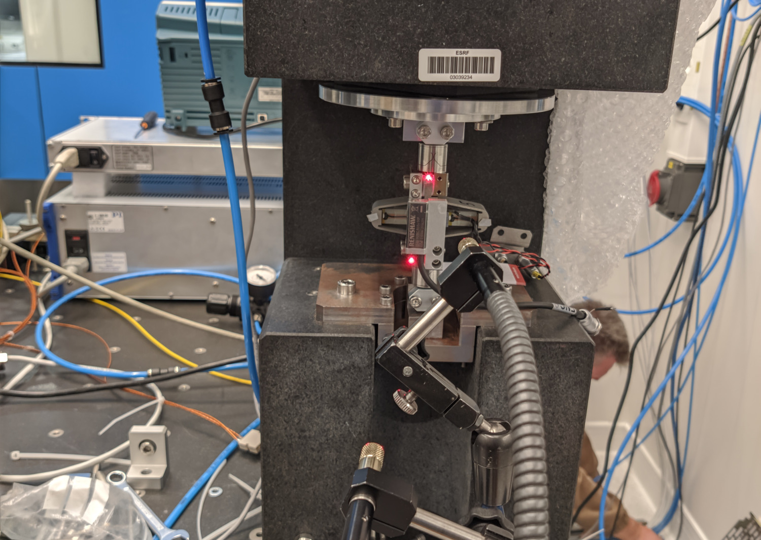
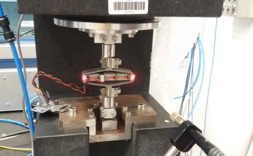
These modes are present when flexible joints are fixed to the ends of the APA300ML. To experimentally measure the frequency of these modes, the struts are mounted (both with and without the encoder). Then, each end of the strut is fixed to a vertically guided stage as shown in Figure ref:fig:test_struts_meas_spur_res_struts_1_enc.

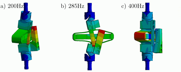
From a Finite Element Model of the struts, it have been found that three main resonances are foreseen to be problematic for the control of the APA300ML (Figure ref:fig:test_struts_mode_shapes):

• Mode in X-bending at 189Hz
• Mode in Y-bending at 285Hz
• Mode in Z-torsion at 400Hz

Measurement Setup

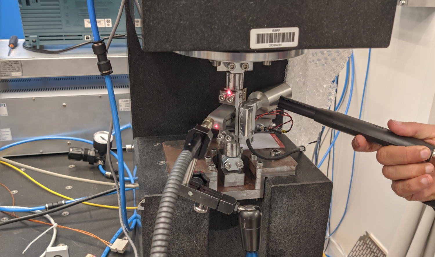
A Laser vibrometer is measuring the difference of motion between two points (Figure ref:fig:test_struts_meas_spur_res_struts_1_enc). The APA is excited with an instrumented hammer and the transfer function from the hammer to the measured rotation is computed.

The instrumentation used are:

• Laser Doppler Vibrometer Polytec OFV512
• Instrumented hammer

The "X-bending" mode is measured as shown in Figure ref:fig:test_struts_meas_spur_res_struts_1_enc. The "Y-bending" mode is measured as shown in Figure ref:fig:test_struts_meas_spur_res_struts_2 with the encoder and in Figure ref:fig:test_struts_meas_spur_res_struts_2_encoder with the encoder. Finally, the "Z-torsion" is measured as shown in Figure ref:fig:test_struts_meas_spur_res_struts_3.

Without Encoder

When the encoder is not fixed to the strut, the obtained FRF are shown in Figure ref:fig:test_struts_spur_res_frf.

Obtained FRF for the struts without the encoder

With Encoder

Then, one encoder is fixed to the strut and the FRF are measured again and shown in Figure ref:fig:test_struts_spur_res_frf_enc.

Obtained FRF for the struts with encoder

Conclusion

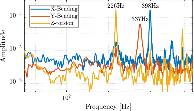
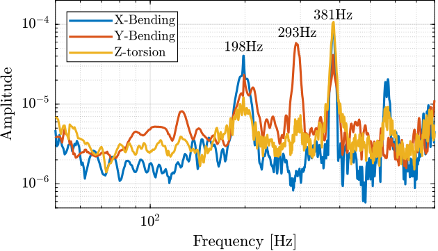
Table ref:tab:test_struts_spur_mode_freqs summarizes the measured resonance frequencies as well as the computed ones using the Finite Element Model.

From the values in Table ref:tab:test_struts_spur_mode_freqs, it is shown that:

• the resonance frequencies of the 3 modes are only slightly increasing when the encoder is removed
• the computed resonance frequencies from the FEM are very close to the measured one when the encoder is fixed to the strut

Mode	Struts (FEM)	Struts (exp)	Plates (exp)
X-Bending	189Hz	198Hz	226Hz
Y-Bending	285Hz	293Hz	337Hz
Z-Torsion	400Hz	381Hz	398Hz

Dynamical measurements

<<sec:test_struts_dynamical_meas>>

Introduction   ignore

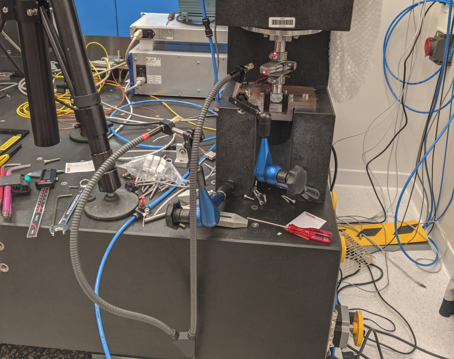
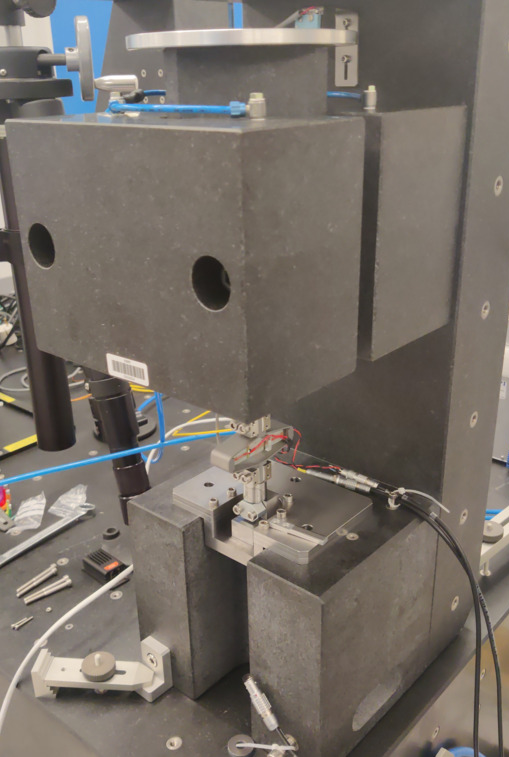
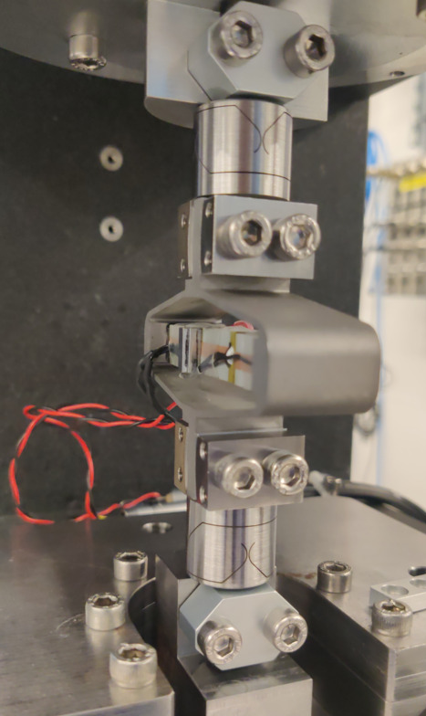
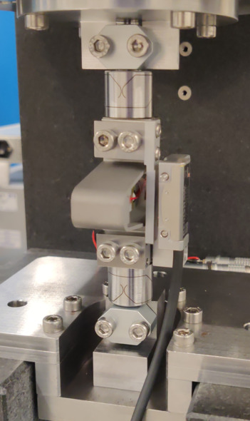
The bench is shown in Figure ref:fig:test_struts_bench_leg_overview. Measurements are performed either when no encoder is fixed to the strut (Figure ref:fig:test_struts_bench_leg_front) or when one encoder is fixed to the strut (Figure ref:fig:test_struts_bench_leg_coder).

Experimental setup to measured the dynamics of the struts.

First, only one strut is measured in details (Section ref:ssec:test_struts_meas_strut_1), and then all the struts are measured and compared (Section ref:ssec:test_struts_meas_all_struts).

Measurement on Strut 1

<<ssec:test_struts_meas_strut_1>>

Introduction   ignore

Measurements are first performed on one of the strut that contains:

• the Amplified Piezoelectric Actuator (APA) number 1
• flexible joints 1 and 2

In Section ref:sec:meas_strut_1_no_encoder, the dynamics of the strut is measured without the encoder attached to it. Then in Section ref:sec:meas_strut_1_encoder, the encoder is attached to the struts, and the dynamic is identified.

Without Encoder

<<sec:meas_strut_1_no_encoder>>

FRF Identification - Setup

Similarly to what was done for the identification of the APA, the identification is performed in three steps:

1. White noise excitation with small amplitude. This is used to determine the main resonance of the system.
2. Sweep sine excitation with the amplitude lowered around the resonance. The sweep sine is from 10Hz to 400Hz.
3. High frequency noise. The noise is band-passed between 300Hz and 2kHz.

Then, the result of the second identification is used between 10Hz and 350Hz and the result of the third identification if used between 350Hz and 2kHz.

%% Load Data
leg_sweep    = load('frf_data_leg_1_sweep.mat', 't', 'Va', 'Vs', 'de', 'da');
leg_noise_hf = load('frf_data_leg_1_noise_hf.mat', 't', 'Va', 'Vs', 'de', 'da');

The time is the same for all measurements.

%% Time vector
t = leg_sweep.t - leg_sweep.t(1) ; % Time vector [s]

%% Sampling frequency/time
Ts = 1e-4; % Sampling Time [s]
Fs = 1/Ts; % Sampling Frequency [Hz]
Nfft = floor(1/Ts);
win = hanning(Nfft);
Noverlap = floor(Nfft/2);

We get the frequency vector that will be the same for all the frequency domain analysis.

% Only used to have the frequency vector "f"
[~, f] = tfestimate(leg_sweep.Va, leg_sweep.de, win, Noverlap, Nfft, 1/Ts);
i_lf = f <= 350; % Indices used for the low frequency
i_hf = f >  350; % Indices used for the low frequency

FRF Identification - Interferometer

In this section, the dynamics from the excitation voltage $V_a$ to the interferometer $d_a$ is identified.

We compute the coherence for 2nd and 3rd identification and combine them.

%% Compute the coherence for both excitation signals
[int_coh_sweep, ~]    = mscohere(leg_sweep.Va,    leg_sweep.da,    win, Noverlap, Nfft, 1/Ts);
[int_coh_noise_hf, ~] = mscohere(leg_noise_hf.Va, leg_noise_hf.da, win, Noverlap, Nfft, 1/Ts);

%% Combine the coherence
int_coh = [int_coh_sweep(i_lf); int_coh_noise_hf(i_hf)];

The combined coherence is shown in Figure ref:fig:strut_1_frf_dvf_plant_coh, and is found to be very good up to at least 1kHz.

Obtained coherence for the plant from $V_a$ to $d_a$

The transfer function from $V_a$ to the interferometer measured displacement $d_a$ is estimated and shown in Figure ref:fig:strut_1_frf_dvf_plant_tf.

%% Compute FRF function from Va to da
[frf_sweep, ~]    = tfestimate(leg_sweep.Va,    leg_sweep.da,    win, Noverlap, Nfft, 1/Ts);
[frf_noise_hf, ~] = tfestimate(leg_noise_hf.Va, leg_noise_hf.da, win, Noverlap, Nfft, 1/Ts);

%% Combine the FRF
int_frf = [frf_sweep(i_lf); frf_noise_hf(i_hf)];

Estimated FRF for the DVF plant (transfer function from $V_a$ to the interferometer $d_a$)

FRF Identification - IFF

In this section, the dynamics from $V_a$ to $V_s$ is identified.

First the coherence is computed and shown in Figure ref:fig:strut_1_frf_iff_plant_coh. The coherence is very nice from 10Hz to 2kHz. It is only dropping near a zeros at 40Hz, and near the resonance at 95Hz (the excitation amplitude being lowered).

%% Compute the coherence for both excitation signals
[iff_coh_sweep, ~]    = mscohere(leg_sweep.Va,    leg_sweep.Vs,    win, Noverlap, Nfft, 1/Ts);
[iff_coh_noise_hf, ~] = mscohere(leg_noise_hf.Va, leg_noise_hf.Vs, win, Noverlap, Nfft, 1/Ts);

%% Combine the coherence
iff_coh = [iff_coh_sweep(i_lf); iff_coh_noise_hf(i_hf)];

Obtained coherence for the IFF plant

Then the FRF are estimated and shown in Figure ref:fig:strut_1_frf_iff_plant_tf

%% Compute the FRF
[frf_sweep,    ~] = tfestimate(leg_sweep.Va,    leg_sweep.Vs,    win, Noverlap, Nfft, 1/Ts);
[frf_noise_hf, ~] = tfestimate(leg_noise_hf.Va, leg_noise_hf.Vs, win, Noverlap, Nfft, 1/Ts);

%% Combine the FRF
iff_frf = [frf_sweep(i_lf); frf_noise_hf(i_hf)];

#+caption:Identified IFF Plant for the Strut 1

With Encoder

<<sec:meas_strut_1_encoder>>

Introduction   ignore

Now the encoder is fixed to the strut and the identification is performed.

Measurement Data

The measurements are loaded.

%% Load data
leg_enc_sweep    = load(sprintf('frf_data_leg_coder_badly_align_%i_noise.mat',    1), 't', 'Va', 'Vs', 'de', 'da');
leg_enc_noise_hf = load(sprintf('frf_data_leg_coder_badly_align_%i_noise_hf.mat', 1), 't', 'Va', 'Vs', 'de', 'da');

FRF Identification - Interferometer

In this section, the dynamics from $V_a$ to $d_a$ is identified.

First, the coherence is computed and shown in Figure ref:fig:strut_1_int_with_enc_frf_dvf_plant_coh.

%% Compute the coherence for both excitation signals
[int_coh_sweep, ~]    = mscohere(leg_enc_sweep.Va,    leg_enc_sweep.da,    win, Noverlap, Nfft, 1/Ts);
[int_coh_noise_hf, ~] = mscohere(leg_enc_noise_hf.Va, leg_enc_noise_hf.da, win, Noverlap, Nfft, 1/Ts);

%% Combine the coherinte
int_coh = [int_coh_sweep(i_lf); int_coh_noise_hf(i_hf)];

Obtained coherence for the plant from $V_a$ to $d_a$

Then the FRF are computed and shown in Figure ref:fig:strut_1_int_with_enc_frf_dvf_plant_tf.

%% Compute FRF function from Va to da
[frf_sweep, ~]    = tfestimate(leg_enc_sweep.Va,    leg_enc_sweep.da,    win, Noverlap, Nfft, 1/Ts);
[frf_noise_hf, ~] = tfestimate(leg_enc_noise_hf.Va, leg_enc_noise_hf.da, win, Noverlap, Nfft, 1/Ts);

%% Combine the FRF
int_with_enc_frf = [frf_sweep(i_lf); frf_noise_hf(i_hf)];

Estimated FRF for the DVF plant (transfer function from $V_a$ to the encoder $d_e$)

The obtained FRF is very close to the one that was obtained when no encoder was fixed to the struts as shown in Figure ref:fig:strut_leg_compare_int_frf.

Comparison of the measured FRF from $V_a$ to $d_a$ with and without the encoders fixed to the struts

FRF Identification - Encoder

In this section, the dynamics from $V_a$ to $d_e$ (encoder) is identified.

The coherence is computed and shown in Figure ref:fig:strut_1_enc_frf_dvf_plant_coh.

%% Compute the coherence for both excitation signals
[enc_coh_sweep, ~]    = mscohere(leg_enc_sweep.Va,    leg_enc_sweep.de,    win, Noverlap, Nfft, 1/Ts);
[enc_coh_noise_hf, ~] = mscohere(leg_enc_noise_hf.Va, leg_enc_noise_hf.de, win, Noverlap, Nfft, 1/Ts);

%% Combine the coherence
enc_coh = [enc_coh_sweep(i_lf); enc_coh_noise_hf(i_hf)];

Obtained coherence for the plant from $V_a$ to $d_e$ and from $V_a$ to $d_a$

The FRF from $V_a$ to the encoder measured displacement $d_e$ is computed and shown in Figure ref:fig:strut_1_enc_frf_dvf_plant_tf.

%% Compute FRF function from Va to da
[frf_sweep, ~]    = tfestimate(leg_enc_sweep.Va,    leg_enc_sweep.de,    win, Noverlap, Nfft, 1/Ts);
[frf_noise_hf, ~] = tfestimate(leg_enc_noise_hf.Va, leg_enc_noise_hf.de, win, Noverlap, Nfft, 1/Ts);

%% Combine the FRF
enc_frf = [frf_sweep(i_lf); frf_noise_hf(i_hf)];

Estimated FRF for the DVF plant (transfer function from $V_a$ to the encoder $d_e$)

The transfer functions from $V_a$ to $d_e$ (encoder) and to $d_a$ (interferometer) are compared in Figure ref:fig:strut_1_comp_enc_int.

Comparison of the transfer functions from excitation voltage $V_a$ to either the encoder $d_e$ or the interferometer $d_a$

The dynamics from the excitation voltage $V_a$ to the measured displacement by the encoder $d_e$ presents much more complicated behavior than the transfer function to the displacement as measured by the Interferometer (compared in Figure ref:fig:strut_1_comp_enc_int). It will be further investigated why the two dynamics as so different and what are causing all these resonances.

APA Resonances Frequency

As shown in Figure ref:fig:strut_1_spurious_resonances, we can clearly see three spurious resonances at 197Hz, 290Hz and 376Hz.

Magnitude of the transfer function from excitation voltage $V_a$ to encoder measurement $d_e$. The frequency of the resonances are noted.

These resonances correspond to parasitic resonances of the strut itself.

They are very close to what was estimated using a finite element model of the strut (Figure ref:fig:test_struts_mode_shapes):

• Mode in X-bending at 189Hz
• Mode in Y-bending at 285Hz
• Mode in Z-torsion at 400Hz

The resonances seen by the encoder in Figure ref:fig:strut_1_spurious_resonances are indeed corresponding to the modes of the strut as shown in Figure ref:fig:test_struts_mode_shapes.

FRF Identification - Force Sensor

In this section, the dynamics from $V_a$ to $V_s$ is identified.

First the coherence is computed and shown in Figure ref:fig:strut_1_frf_iff_with_enc_plant_coh. The coherence is very nice from 10Hz to 2kHz. It is only dropping near a zeros at 40Hz, and near the resonance at 95Hz (the excitation amplitude being lowered).

%% Compute the coherence for both excitation signals
[iff_coh_sweep, ~]    = mscohere(leg_enc_sweep.Va,    leg_enc_sweep.Vs,    win, Noverlap, Nfft, 1/Ts);
[iff_coh_noise_hf, ~] = mscohere(leg_enc_noise_hf.Va, leg_enc_noise_hf.Vs, win, Noverlap, Nfft, 1/Ts);

%% Combine the coherence
iff_coh = [iff_coh_sweep(i_lf); iff_coh_noise_hf(i_hf)];

Obtained coherence for the IFF plant

Then the FRF are estimated and shown in Figure ref:fig:strut_1_enc_frf_iff_plant_tf

%% Compute FRF function from Va to da
[frf_sweep, ~]    = tfestimate(leg_enc_sweep.Va,    leg_enc_sweep.Vs,    win, Noverlap, Nfft, 1/Ts);
[frf_noise_hf, ~] = tfestimate(leg_enc_noise_hf.Va, leg_enc_noise_hf.Vs, win, Noverlap, Nfft, 1/Ts);

%% Combine the FRF
iff_with_enc_frf = [frf_sweep(i_lf); frf_noise_hf(i_hf)];

#+caption:Identified IFF Plant

Let's now compare the IFF plants whether the encoders are fixed to the APA or not (Figure ref:fig:strut_1_frf_iff_comp_enc).

Effect of the encoder on the IFF plant

The transfer function from the excitation voltage $V_a$ to the generated voltage $V_s$ by the sensor stack is not influence by the fixation of the encoder. This means that the IFF control strategy should be as effective whether or not the encoders are fixed to the struts.

TODO Non-Minimum phase zero?

In order to determine if the complex conjugate zero of Figure ref:fig:strut_1_enc_frf_iff_plant_tf is minimum phase or non-minimum phase, longer measurements are performed.

long_sweep = load('frf_struts_align_3_sweep_long.mat', 't', 'Va', 'Vs');
long_noise = load('frf_struts_align_3_noise_long.mat', 't', 'Va', 'Vs');

Ts = (long_sweep.t(end) - long_sweep.t(1))/(length(long_sweep.t)-1); % Sampling Time [s]
Fs = 1/Ts;

win = hanning(ceil(50*Fs)); % Hannning Windows

%% Transfer function estimation
[coh_sweep, f] = mscohere(long_sweep.Va, long_sweep.Vs, win, Noverlap, Nfft, 1/Ts);
[coh_noise, ~] = mscohere(long_noise.Va, long_noise.Vs, win, Noverlap, Nfft, 1/Ts);

Remove time delay

long_sweep.Va(end) = [];
long_noise.Va(end) = [];

long_sweep.Vs(1) = [];
long_noise.Vs(1) = [];

%% Transfer function estimation
[frf_sweep, f] = tfestimate(long_sweep.Va, long_sweep.Vs, win, Noverlap, Nfft, 1/Ts);
[frf_noise, ~] = tfestimate(long_noise.Va, long_noise.Vs, win, Noverlap, Nfft, 1/Ts);

Comparison of all the Struts

<<ssec:test_struts_meas_all_struts>>

Introduction   ignore

Now all struts are measured using the same procedure and test bench as in Section ref:sec:meas_strut_1.

FRF Identification - Setup

The identification of the struts dynamics is performed in two steps:

1. The excitation signal is a white noise with small amplitude. This is used to estimate the low frequency dynamics.
2. Then a high frequency noise band-passed between 300Hz and 2kHz is used to estimate the high frequency dynamics.

Then, the result of the first identification is used between 10Hz and 350Hz and the result of the second identification if used between 350Hz and 2kHz.

Here are the leg numbers that have been measured.

%% Numnbers of the measured legs
leg_nums = [1 2 3 4 5];

The data are loaded for both the first and second identification:

%% First identification (low frequency noise)
leg_noise = {};
for i = 1:length(leg_nums)
    leg_noise(i) = {load(sprintf('frf_data_leg_coder_%i_noise.mat', leg_nums(i)), 't', 'Va', 'Vs', 'de', 'da')};
end

%% Second identification (high frequency noise)
leg_noise_hf = {};
for i = 1:length(leg_nums)
    leg_noise_hf(i) = {load(sprintf('frf_data_leg_coder_%i_noise_hf.mat', leg_nums(i)), 't', 'Va', 'Vs', 'de', 'da')};
end

The time is the same for all measurements.

%% Time vector
t = leg_noise{1}.t - leg_noise{1}.t(1) ; % Time vector [s]

%% Sampling
Ts = (t(end) - t(1))/(length(t)-1); % Sampling Time [s]
Fs = 1/Ts; % Sampling Frequency [Hz]

Then we defined a "Hanning" windows that will be used for the spectral analysis:

win = hanning(ceil(0.5*Fs)); % Hannning Windows

We get the frequency vector that will be the same for all the frequency domain analysis.

% Only used to have the frequency vector "f"
[~, f] = tfestimate(leg_noise{1}.Va, leg_noise{1}.de, win, Noverlap, Nfft, 1/Ts);
i_lf = f <= 350;
i_hf = f >  350;

FRF Identification - Encoder

In this section, the dynamics from $V_a$ to $d_e$ (encoder) is identified.

The coherence is computed and shown in Figure ref:fig:struts_frf_dvf_plant_coh for all the measured struts.

%% Coherence computation
coh_enc = zeros(length(f), length(leg_nums));
for i = 1:length(leg_nums)
    [coh_lf, ~] = mscohere(leg_noise{i}.Va,    leg_noise{i}.de,    win, Noverlap, Nfft, 1/Ts);
    [coh_hf, ~] = mscohere(leg_noise_hf{i}.Va, leg_noise_hf{i}.de, win, Noverlap, Nfft, 1/Ts);
    coh_enc(:, i) = [coh_lf(i_lf); coh_hf(i_hf)];
end

Obtained coherence for the plant from $V_a$ to $d_e$

Then, the transfer function from the DAC output voltage $V_a$ to the measured displacement by the encoder $d_e$ is computed:

%% Transfer function estimation
enc_frf = zeros(length(f), length(leg_nums));

for i = 1:length(leg_nums)
    [frf_lf, ~] = tfestimate(leg_noise{i}.Va,    leg_noise{i}.de,    win, Noverlap, Nfft, 1/Ts);
    [frf_hf, ~] = tfestimate(leg_noise_hf{i}.Va, leg_noise_hf{i}.de, win, Noverlap, Nfft, 1/Ts);
    enc_frf(:, i) = [frf_lf(i_lf); frf_hf(i_hf)];
end

The obtained transfer functions are shown in Figure ref:fig:struts_frf_dvf_plant_tf.

Estimated FRF for the DVF plant (transfer function from $V_a$ to the encoder $d_e$)

There is a very large variability of the dynamics as measured by the encoder as shown in Figure ref:fig:struts_frf_dvf_plant_tf. Even-though the same peaks are seen for all of the struts (95Hz, 200Hz, 300Hz, 400Hz), the amplitude of the peaks are not the same. Moreover, the location or even the presence of complex conjugate zeros is changing from one strut to the other.

All of this will be explained in Section ref:sec:simscape_bench_struts thanks to the Simscape model.

FRF Identification - Interferometer

In this section, the dynamics from $V_a$ to $d_a$ (interferometer) is identified.

The coherence is computed and shown in Figure ref:fig:struts_frf_int_plant_coh.

%% Coherence computation
coh_int = zeros(length(f), length(leg_nums));
for i = 1:length(leg_nums)
    [coh_lf, ~] = mscohere(leg_noise{i}.Va,    leg_noise{i}.da,    win, Noverlap, Nfft, 1/Ts);
    [coh_hf, ~] = mscohere(leg_noise_hf{i}.Va, leg_noise_hf{i}.da, win, Noverlap, Nfft, 1/Ts);
    coh_int(:, i) = [coh_lf(i_lf); coh_hf(i_hf)];
end

Obtained coherence for the plant from $V_a$ to $d_e$

Then, the transfer function from the DAC output voltage $V_a$ to the measured displacement by the Attocube is computed for all the struts and shown in Figure ref:fig:struts_frf_int_plant_tf. All the struts are giving very similar FRF.

%% Transfer function estimation
int_frf = zeros(length(f), length(leg_nums));
for i = 1:length(leg_nums)
    [frf_lf, ~] = tfestimate(leg_noise{i}.Va,    leg_noise{i}.da,    win, Noverlap, Nfft, 1/Ts);
    [frf_hf, ~] = tfestimate(leg_noise_hf{i}.Va, leg_noise_hf{i}.da, win, Noverlap, Nfft, 1/Ts);
    int_frf(:, i) = [frf_lf(i_lf); frf_hf(i_hf)];
end

Estimated FRF for the DVF plant (transfer function from $V_a$ to the encoder $d_e$)

FRF Identification - Force Sensor

In this section, the dynamics from $V_a$ to $V_s$ is identified.

First the coherence is computed and shown in Figure ref:fig:struts_frf_iff_plant_coh.

%% Coherence
coh_iff = zeros(length(f), length(leg_nums));
for i = 1:length(leg_nums)
    [coh_lf, ~] = mscohere(leg_noise{i}.Va,    leg_noise{i}.Vs,    win, Noverlap, Nfft, 1/Ts);
    [coh_hf, ~] = mscohere(leg_noise_hf{i}.Va, leg_noise_hf{i}.Vs, win, Noverlap, Nfft, 1/Ts);
    coh_iff(:, i) = [coh_lf(i_lf); coh_hf(i_hf)];
end

Obtained coherence for the IFF plant

Then the FRF are estimated and shown in Figure ref:fig:struts_frf_iff_plant_tf. They are also shown all to be very similar.

%% FRF estimation of the transfer function from Va to Vs
iff_frf = zeros(length(f), length(leg_nums));
for i = 1:length(leg_nums)
    [frf_lf, ~] = tfestimate(leg_noise{i}.Va,    leg_noise{i}.Vs,    win, Noverlap, Nfft, 1/Ts);
    [frf_hf, ~] = tfestimate(leg_noise_hf{i}.Va, leg_noise_hf{i}.Vs, win, Noverlap, Nfft, 1/Ts);
    iff_frf(:, i) = [frf_lf(i_lf); frf_hf(i_hf)];
end

#+caption:Identified IFF Plant

Misalignment of the APA and flexible joints

The misalignment between the two flexible joints and the APA has been measured for all the struts:

• the strut is fixed to the mounting bench
• using an indicator, the height difference from the flexible joints and the APA is measured both for the top and bottom joints and on both sides
• then it is possible to obtain the misalignment for both flexible joints

The raw measurements are shown in Table ref:tab:meas_misalignment_struts_raw.

As the flexible joint's "thickness" is 1mm larger than the APA "thickness", ideally (i.e. if it were perfectly centered) we would measure -0.50mm each time.

strut_nums = [1, 2, 3, 4, 5];

%             R Top  B Top  R Bot  B Bot
strut_align = [[-0.40, -0.60, -0.16, -0.82]   % Strut 1
               [-0.67, -0.30, -0.34, -0.63]   % Strut 2
               [-0.07, -0.88, -0.16, -0.79]   % Strut 3
               [-0.48, -0.46,  0.07, -1.00]   % Strut 4
               [-0.33, -0.64, -0.48, -0.52]]; % Strut 5

Strut	R Top	B Top	R Bot	B Bot
1	-0.4	-0.6	-0.16	-0.82
2	-0.67	-0.3	-0.34	-0.63
3	-0.07	-0.88	-0.16	-0.79
4	-0.48	-0.46	0.07	-1.0
5	-0.33	-0.64	-0.48	-0.52

Also, the sum of the measured distances on each side should be 1mm (equal to the thickness difference between the flexible joint and the APA). This is verified in Table ref:tab:meas_misalignment_struts_thickness.

Strut	Top	Bot
1	-1.0	-0.98
2	-0.97	-0.97
3	-0.95	-0.95
4	-0.94	-0.93
5	-0.97	-1.0

The differences of the measured distances on each side corresponds to the misalignment on that same side (Table ref:tab:meas_misalignment_struts_results).

Strut	Top	Bot
1	0.1	0.33
2	-0.185	0.145
3	0.405	0.315
4	-0.01	0.535
5	0.155	0.02

The misalignment of the APA and flexible joints is quite large and variable from one strut to the other.

Conclusion

All the struts are giving very consistent behavior from the excitation voltage $V_a$ to the force sensor generated voltage $V_s$ and to the interferometer measured displacement $d_a$. However, the dynamics from $V_a$ to the encoder measurement $d_e$ is much more complex and variable from one strut to the other most likely due to poor alignment of the APA with respect to the flexible joints.

The measured FRF are now saved for further use.

%% Save the estimated FRF for further analysis
save('mat/meas_struts_frf.mat', 'f', 'Ts', 'enc_frf', 'int_frf', 'iff_frf', 'leg_nums', 'apa_align');

Comparison of all the (re-aligned) Struts

<<sec:test_struts_meas_all_aligned_struts>>

Introduction   ignore

The struts are re-aligned and measured using the same test bench.

Measured misalignment of the APA and flexible joints

The misalignment between the APA and the flexible joints are measured.

The results are defined below and summarized in Table ref:tab:meas_misalignment_struts_new_raw.

%               R Top  B Top  R Bot  B Bot
strut_align = [[-0.54, -0.50, -0.50, -0.52]   % strut 1
               [-0.44, -0.55, -0.49, -0.49]   % strut 2
               [-0.48, -0.50, -0.50, -0.46]   % strut 3
               [-0.45, -0.51, -0.51, -0.45]   % strut 4
               [-0.50, -0.50, -0.50, -0.50]   % strut 5
               [-0.50, -0.49, -0.43, -0.54]]; % strut 6

Strut	R Top	B Top	R Bot	B Bot
1	-0.54	-0.5	-0.5	-0.52
2	-0.44	-0.55	-0.49	-0.49
3	-0.48	-0.5	-0.5	-0.46
4	-0.45	-0.51	-0.51	-0.45
5	-0.5	-0.5	-0.5	-0.5
6	-0.5	-0.49	-0.43	-0.54

Also, the sum of the measured distances on each side should be 1mm (equal to the thickness difference between the flexible joint and the APA). This is verified in Table ref:tab:meas_misalignment_struts_new_thickness.

APA	Top	Bot
1	-1.04	-1.02
2	-0.99	-0.98
4	-0.98	-0.96
5	-0.96	-0.96
6	-1.0	-1.0
8	-0.99	-0.97

The differences of the measured distances on each side corresponds to the misalignment on that same side (Table ref:tab:meas_misalignment_struts_new_results).

APA	Top	Bot
1	-0.02	0.01
2	0.055	0.0
4	0.01	-0.02
5	0.03	-0.03
6	0.0	0.0
8	-0.005	0.055

After using the alignment pins, the misalignment of the APA and flexible joints are much smaller ($< 50\,\mu m$ for all the struts).

FRF Identification - Setup

The excitation signal is a low pass filtered white noise. Both the encoder and the force sensor voltage are measured.

Here are the leg numbers that have been measured.

%% Numnbers of the measured legs
leg_nums = [1 2 3 4 5 6];

%% First identification (low frequency noise)
leg_noise = {};
for i = 1:length(leg_nums)
    leg_noise(i) = {load(sprintf('frf_struts_align_%i_noise.mat', leg_nums(i)), 't', 'Va', 'Vs', 'de')};
end

The time is the same for all measurements.

%% Time vector
t = leg_noise{1}.t - leg_noise{1}.t(1) ; % Time vector [s]

%% Sampling
Ts = (t(end) - t(1))/(length(t)-1); % Sampling Time [s]
Fs = 1/Ts; % Sampling Frequency [Hz]

Then we defined a "Hanning" windows that will be used for the spectral analysis:

win = hanning(ceil(0.5*Fs)); % Hannning Windows

We get the frequency vector that will be the same for all the frequency domain analysis.

% Only used to have the frequency vector "f"
[~, f] = tfestimate(leg_noise{1}.Va, leg_noise{1}.de, win, Noverlap, Nfft, 1/Ts);

FRF Identification - Encoder

In this section, the dynamics from $V_a$ to $d_e$ (encoder) is identified.

The coherence is computed and shown in Figure ref:fig:struts_align_frf_dvf_plant_coh for all the measured struts.

%% Coherence computation
coh_enc = zeros(length(f), length(leg_nums));
for i = 1:length(leg_nums)
    coh_enc(:, i) = mscohere(leg_noise{i}.Va,    leg_noise{i}.de,    win, Noverlap, Nfft, 1/Ts);
end

Obtained coherence for the plant from $V_a$ to $d_e$

Then, the transfer function from the DAC output voltage $V_a$ to the measured displacement by the encoder $d_e$ is computed:

%% Transfer function estimation
enc_frf = zeros(length(f), length(leg_nums));

for i = 1:length(leg_nums)
    enc_frf(:, i) = tfestimate(leg_noise{i}.Va,    leg_noise{i}.de,    win, Noverlap, Nfft, 1/Ts);
end

The obtained transfer functions are shown in Figure ref:fig:struts_align_frf_dvf_plant_tf.

Estimated FRF for the DVF plant (transfer function from $V_a$ to the encoder $d_e$)

Even though the struts are much better aligned, we still observe high variability between the struts for the transfer function from $V_a$ to $d_e$.

FRF Identification - Force Sensor

In this section, the dynamics from $V_a$ to $V_s$ is identified.

First the coherence is computed and shown in Figure ref:fig:struts_frf_iff_plant_coh.

%% Coherence
coh_iff = zeros(length(f), length(leg_nums));
for i = 1:length(leg_nums)
    coh_iff(:, i) = mscohere(leg_noise{i}.Va,    leg_noise{i}.Vs,    win, Noverlap, Nfft, 1/Ts);
end

Obtained coherence for the IFF plant

Then the FRF are estimated and shown in Figure ref:fig:struts_frf_iff_plant_tf. They are also shown all to be very similar.

%% FRF estimation of the transfer function from Va to Vs
iff_frf = zeros(length(f), length(leg_nums));
for i = 1:length(leg_nums)
    iff_frf(:, i) = tfestimate(leg_noise{i}.Va,    leg_noise{i}.Vs,    win, Noverlap, Nfft, 1/Ts);
end

#+caption:Identified IFF Plant

Conclusion

Having the struts well aligned does not change significantly the obtained dynamics.

The measured FRF are now saved for further use.

%% Save the estimated FRF for further analysis
save('mat/meas_struts_frf.mat', 'f', 'Ts', 'enc_frf', 'iff_frf', 'leg_nums', 'strut_align');

Simscape Model

<<sec:test_struts_simscape>>

Introduction   ignore

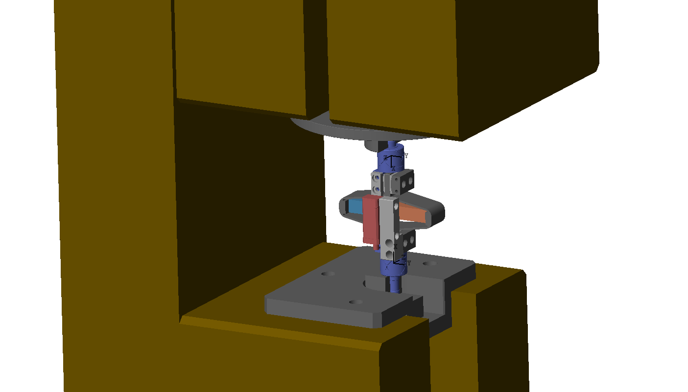
However, now the full strut is put instead of only the APA (see Figure ref:fig:test_struts_simscape_model).

This Simscape model is used to:

• compare the measured FRF with the modelled FRF
• help the correct understanding/interpretation of the results
• tune the model of the struts (APA, flexible joints, encoder)

This study is structured as follow:

• Section ref:sec:struts_comp_2dof: the measured FRF are compared with the 2DoF APA model.
• Section ref:sec:struts_effect_misalignment: the flexible APA model is used, and the effect of a misalignment of the APA and flexible joints is studied. It is found that the misalignment has a large impact on the dynamics from $V_a$ to $d_e$.
• Section ref:sec:struts_effect_joint_stiffness: the effect of the flexible joint's stiffness on the dynamics is studied. It is found that the axial stiffness of the joints has a large impact on the location of the zeros on the transfer function from $V_s$ to $d_e$.

Comparison with the 2-DoF Model

<<sec:struts_comp_2dof>>

First Identification

The strut is initialized with default parameters (optimized parameters identified from previous experiments).

%% Initialize structure containing data for the Simscape model
n_hexapod = struct();
n_hexapod.flex_bot = initializeBotFlexibleJoint('type', '4dof');
n_hexapod.flex_top = initializeTopFlexibleJoint('type', '4dof');
n_hexapod.actuator = initializeAPA('type', '2dof');

The inputs and outputs of the model are defined.

%% Input/Output definition
clear io; io_i = 1;
io(io_i) = linio([mdl, '/Va'], 1, 'openinput');  io_i = io_i + 1; % Actuator Voltage
io(io_i) = linio([mdl, '/Vs'], 1, 'openoutput'); io_i = io_i + 1; % Sensor Voltage
io(io_i) = linio([mdl, '/de'], 1, 'openoutput'); io_i = io_i + 1; % Encoder
io(io_i) = linio([mdl, '/da'], 1, 'openoutput'); io_i = io_i + 1; % Interferometer

The dynamics is identified and shown in Figure ref:fig:strut_bench_model_bode.

%% Run the linearization
Gs = linearize(mdl, io, 0.0, options);
Gs.InputName  = {'Va'};
Gs.OutputName = {'Vs', 'de', 'da'};

Identified transfer function from $V_a$ to $V_s$ and from $V_a$ to $d_e,d_a$ using the simple 2DoF model for the APA

Comparison with the experimental Data

The experimentally measured FRF are loaded.

%% Load measured FRF

%% Add time delay to the Simscape model
Gs = exp(-s*Ts)*Gs;

The FRF from $V_a$ to $d_a$ as well as from $V_a$ to $V_s$ are shown in Figure ref:fig:comp_strut_plant_after_opt and compared with the model. They are both found to match quite well with the model.

Comparison of the measured FRF and the optimized model

The measured FRF from $V_a$ to $d_e$ (encoder) is compared with the model in Figure ref:fig:comp_strut_plant_iff_after_opt.

Comparison of the measured FRF and the optimized model

The 2-DoF model is quite effective in modelling the transfer function from actuator to force sensor and from actuator to interferometer (Figure ref:fig:comp_strut_plant_after_opt). But it is not effective in modeling the transfer function from actuator to encoder (Figure ref:fig:comp_strut_plant_iff_after_opt). This is due to the fact that resonances greatly affecting the encoder reading are not modelled. In the next section, flexible model of the APA will be used to model such resonances.

Comparison with the Flexible Model

<<sec:struts_comp_flexible>>

First Identification

The strut is initialized with default parameters (optimized parameters identified from previous experiments).

%% Initialize structure containing data for the Simscape model
n_hexapod = struct();
n_hexapod.flex_bot = initializeBotFlexibleJoint('type', '4dof');
n_hexapod.flex_top = initializeTopFlexibleJoint('type', '4dof');
n_hexapod.actuator = initializeAPA('type', 'flexible');

The inputs and outputs of the model are defined.

%% Input/Output definition
clear io; io_i = 1;
io(io_i) = linio([mdl, '/Va'], 1, 'openinput');  io_i = io_i + 1; % Actuator Voltage
io(io_i) = linio([mdl, '/Vs'], 1, 'openoutput'); io_i = io_i + 1; % Sensor Voltage
io(io_i) = linio([mdl, '/de'], 1, 'openoutput'); io_i = io_i + 1; % Encoder
io(io_i) = linio([mdl, '/da'], 1, 'openoutput'); io_i = io_i + 1; % Interferometer

The dynamics is identified and shown in Figure ref:fig:strut_bench_model_bode.

%% Run the linearization
Gs = linearize(mdl, io, 0.0, options);
Gs.InputName  = {'Va'};
Gs.OutputName = {'Vs', 'de', 'da'};

Comparison with the experimental Data

The experimentally measured FRF are loaded.

%% Load measured FRF
load('meas_struts_frf.mat', 'f', 'Ts', 'enc_frf', 'int_frf', 'iff_frf', 'leg_nums');

%% Add time delay to the Simscape model
Gs = exp(-s*Ts)*Gs;

The FRF from $V_a$ to $d_a$ as well as from $V_a$ to $V_s$ are shown in Figure ref:fig:comp_strut_plant_after_opt and compared with the model. They are both found to match quite well with the model.

Effect of a misalignment of the APA and flexible joints on the transfer function from actuator to encoder

<<sec:struts_effect_misalignment>>

Introduction   ignore

As shown in Figure ref:fig:struts_frf_dvf_plant_tf, the dynamics from actuator to encoder for all the struts is very different.

This could be explained by a large variability in the alignment of the flexible joints and the APA (at the time, the alignment pins were not used).

Depending on the alignment, the spurious resonances of the struts (Figure ref:fig:test_struts_mode_shapes) can be excited differently.

For instance, consider Figure ref:fig:strut_misalign_schematic where there is a misalignment in the $y$ direction. In such case, the mode at 200Hz is foreseen to be more excited as the misalignment $d_y$ increases and therefore the dynamics from the actuator to the encoder should also change around 200Hz.

If the misalignment is in the $x$ direction, the mode at 285Hz should be more affected whereas a misalignment in the $z$ direction should not affect these resonances.

Such statement is studied in this section.

But first, the measured FRF of the struts are loaded.

%% Load measured FRF of the struts
load('meas_struts_frf.mat', 'f', 'Ts', 'enc_frf', 'int_frf', 'iff_frf', 'leg_nums');

Perfectly aligned APA

Let's first consider that the strut is perfectly mounted such that the two flexible joints and the APA are aligned.

%% Initialize Simscape data
n_hexapod.flex_bot = initializeBotFlexibleJoint('type', '4dof');
n_hexapod.flex_top = initializeTopFlexibleJoint('type', '4dof');
n_hexapod.actuator = initializeAPA('type', 'flexible');

And define the inputs and outputs of the models:

• Input: voltage generated by the DAC
• Output: measured displacement by the encoder

%% Input/Output definition
clear io; io_i = 1;
io(io_i) = linio([mdl, '/Va'],  1, 'openinput');  io_i = io_i + 1; % Actuator Voltage
io(io_i) = linio([mdl, '/de'],  1, 'openoutput'); io_i = io_i + 1; % Encoder
io(io_i) = linio([mdl, '/da'],  1, 'openoutput'); io_i = io_i + 1; % Encoder

The transfer function is identified and shown in Figure ref:fig:comp_enc_frf_align_perfect.

%% Identification
Gs = exp(-s*Ts)*linearize(mdl, io, 0.0, options);
Gs.InputName  = {'Va'};
Gs.OutputName = {'de', 'da'};

From Figure ref:fig:comp_enc_frf_align_perfect, it is clear that:

1. The model with perfect alignment is not matching the measured FRF
2. The mode at 200Hz is not present in the identified dynamics of the Simscape model
3. The measured FRF have different shapes

Comparison of the model with a perfectly aligned APA and flexible joints with the measured FRF from actuator to encoder

Why is the flexible mode of the strut at 200Hz is not seen in the model in Figure ref:fig:comp_enc_frf_align_perfect?

Probably because the presence of this mode is not due because of the "unbalanced" mass of the encoder, but rather because of the misalignment of the APA with respect to the two flexible joints. This will be verified in the next sections.

Effect of a misalignment in y

Let's compute the transfer function from output DAC voltage $V_s$ to the measured displacement by the encoder $d_e$ for several misalignment in the $y$ direction:

%% Considered misalignments
dy_aligns = [-0.5, -0.1, 0, 0.1, 0.5]*1e-3; % [m]

%% Transfer functions from u to de for all the misalignment in y direction
Gs_align = {zeros(length(dy_aligns), 1)};

for i = 1:length(dy_aligns)
    n_hexapod.actuator = initializeAPA('type', 'flexible', 'd_align', [0; dy_aligns(i); 0]);

    G = exp(-s*Ts)*linearize(mdl, io, 0.0, options);
    G.InputName  = {'Va'};
    G.OutputName = {'de'};

    Gs_align(i) = {G};
end

The obtained dynamics are shown in Figure ref:fig:effect_misalignment_y.

Effect of a misalignement in the $y$ direction

The alignment of the APA with the flexible joints as a huge influence on the dynamics from actuator voltage to measured displacement by the encoder. The misalignment in the $y$ direction mostly influences:

• the presence of the flexible mode at 200Hz

• the location of the complex conjugate zero between the first two resonances:

  • if $d_y < 0$: there is no zero between the two resonances and possibly not even between the second and third ones
  • if $d_y > 0$: there is a complex conjugate zero between the first two resonances
• the location of the high frequency complex conjugate zeros at 500Hz (secondary effect, as the axial stiffness of the joint also has large effect on the position of this zero)

Effect of a misalignment in x

Let's compute the transfer function from output DAC voltage to the measured displacement by the encoder for several misalignment in the $x$ direction:

%% Considered misalignments
dx_aligns = [-0.1, -0.05, 0, 0.05, 0.1]*1e-3; % [m]

%% Transfer functions from u to de for all the misalignment in x direction
Gs_align = {zeros(length(dx_aligns), 1)};

for i = 1:length(dx_aligns)
    n_hexapod.actuator = initializeAPA('type', 'flexible', 'd_align', [dx_aligns(i); 0; 0]);

    G = exp(-s*Ts)*linearize(mdl, io, 0.0, options);
    G.InputName  = {'Va'};
    G.OutputName = {'de'};

    Gs_align(i) = {G};
end

The obtained dynamics are shown in Figure ref:fig:effect_misalignment_x.

Effect of a misalignement in the $x$ direction

The misalignment in the $x$ direction mostly influences the presence of the flexible mode at 300Hz.

Find the misalignment of each strut

From the previous analysis on the effect of a $x$ and $y$ misalignment, it is possible to estimate the $x,y$ misalignment of the measured struts.

The misalignment that gives the best match for the FRF are defined below.

%% Tuned misalignment [m]
d_aligns = [[-0.05,  -0.3,  0];
            [ 0,      0.5,  0];
            [-0.1,   -0.3,  0];
            [ 0,      0.3,  0];
            [-0.05,   0.05, 0]]'*1e-3;

For each misalignment, the dynamics from the DAC voltage to the encoder measurement is identified.

%% Idenfity the transfer function from actuator to encoder for all cases
Gs_align = {zeros(size(d_aligns,2), 1)};

for i = 1:5
    n_hexapod.actuator = initializeAPA('type', 'flexible', 'd_align_top', d_aligns(:,i), 'd_align_bot', d_aligns(:,i));

    G = exp(-s*Ts)*linearize(mdl, io, 0.0, options);
    G.InputName  = {'Va'};
    G.OutputName = {'de', 'da'};

    Gs_align(i) = {G};
end

The results are shown in Figure ref:fig:comp_all_struts_corrected_misalign.

Comparison (model and measurements) of the FRF from DAC voltage u to measured displacement by the encoders for all the struts

By tuning the misalignment of the APA with respect to the flexible joints, it is possible to obtain a good fit between the model and the measurements (Figure ref:fig:comp_all_struts_corrected_misalign).

If encoders are to be used when fixed on the struts, it is therefore very important to properly align the APA and the flexible joints when mounting the struts.

In the future, a "pin" will be used to better align the APA with the flexible joints. We can expect the amplitude of the spurious resonances to decrease.

Effect of flexible joint's characteristics

<<sec:struts_effect_joint_stiffness>>

Introduction   ignore

As the struts are composed of one APA and two flexible joints, it is obvious that the flexible joint characteristics will change the dynamic behavior of the struts.

Using the Simscape model, the effect of the flexible joint's characteristics on the dynamics as measured on the test bench are studied:

• Section ref:sec:struts_effect_bending_stiff_joints: the effects of a change of bending stiffness is studied
• Section ref:sec:struts_effect_axial_stiff_joints: the effects of a change of axial stiffness is studied
• Section ref:sec:struts_effect_bending_damping_joints: the effects of a change of bending damping is studied

The studied dynamics is between $V_a$ and the encoder displacement $d_e$.

%% Input/Output definition
clear io; io_i = 1;
io(io_i) = linio([mdl, '/Va'],  1, 'openinput');  io_i = io_i + 1; % Actuator Voltage
io(io_i) = linio([mdl, '/de'],  1, 'openoutput'); io_i = io_i + 1; % Encoder

Effect of bending stiffness of the flexible joints

<<sec:struts_effect_bending_stiff_joints>>

Let's initialize an APA which is a little bit misaligned.

%% APA Initialization
n_hexapod.actuator = initializeAPA('type', 'flexible', 'd_align', [0.1e-3; 0.5e-3; 0]);

The bending stiffnesses for which the dynamics is identified are defined below.

%% Tested bending stiffnesses [Nm/rad]
kRs = [3, 4, 5, 6, 7];

Then the identification is performed for all the values of the bending stiffnesses.

%% Idenfity the transfer function from actuator to encoder for all bending stiffnesses
Gs = {zeros(length(kRs), 1)};

for i = 1:length(kRs)
    n_hexapod.flex_bot = initializeBotFlexibleJoint(...
        'type', '4dof', ...
        'kRx', kRs(i), ...
        'kRy', kRs(i));
    n_hexapod.flex_top = initializeTopFlexibleJoint(...
        'type', '4dof', ...
        'kRx', kRs(i), ...
        'kRy', kRs(i));

    G = exp(-s*Ts)*linearize(mdl, io, 0.0, options);
    G.InputName  = {'Va'};
    G.OutputName = {'de'};

    Gs(i) = {G};
end

The obtained dynamics from DAC voltage to encoder measurements are compared in Figure ref:fig:effect_enc_bending_stiff.

Dynamics from DAC output to encoder for several bending stiffnesses

The bending stiffness of the joints has little impact on the transfer function from $V_a$ to $d_e$.

Effect of axial stiffness of the flexible joints

<<sec:struts_effect_axial_stiff_joints>>

The axial stiffnesses for which the dynamics is identified are defined below.

%% Tested axial stiffnesses [N/m]
kzs = [5e7 7.5e7 1e8 2.5e8];

Then the identification is performed for all the values of the bending stiffnesses.

%% Idenfity the transfer function from actuator to encoder for all bending stiffnesses
Gs = {zeros(length(kzs), 1)};

for i = 1:length(kzs)
    n_hexapod.flex_bot = initializeBotFlexibleJoint(...
        'type', '4dof', ...
        'kz', kzs(i));
    n_hexapod.flex_top = initializeTopFlexibleJoint(...
        'type', '4dof', ...
        'kz', kzs(i));

    G = exp(-s*Ts)*linearize(mdl, io, 0.0, options);
    G.InputName  = {'Va'};
    G.OutputName = {'de'};

    Gs(i) = {G};
end

The obtained dynamics from DAC voltage to encoder measurements are compared in Figure ref:fig:effect_enc_axial_stiff.

Dynamics from DAC output to encoder for several axial stiffnesses

The axial stiffness of the flexible joint has a large impact on the frequency of the complex conjugate zero. Using the measured FRF on the test-bench, if is therefore possible to estimate the axial stiffness of the flexible joints from the location of the zero.

This method gives nice match between the measured FRF and the one extracted from the simscape model, however it could give not so accurate values of the joint's axial stiffness as other factors are also influencing the location of the zero.

Using this method, an axial stiffness of $70 N/\mu m$ is found to give good results (and is reasonable based on the finite element models).

Effect of bending damping

<<sec:struts_effect_bending_damping_joints>> Now let's study the effect of the bending damping of the flexible joints.

The tested bending damping are defined below:

%% Tested bending dampings [Nm/(rad/s)]
cRs = [1e-3, 5e-3, 1e-2, 5e-2, 1e-1];

Then the identification is performed for all the values of the bending damping.

%% Idenfity the transfer function from actuator to encoder for all bending dampins
Gs = {zeros(length(cRs), 1)};

for i = 1:length(cRs)
    n_hexapod.flex_bot = initializeBotFlexibleJoint(...
        'type', '4dof', ...
        'cRx', cRs(i), ...
        'cRy', cRs(i));
    n_hexapod.flex_top = initializeTopFlexibleJoint(...
        'type', '4dof', ...
        'cRx', cRs(i), ...
        'cRy', cRs(i));

    G = exp(-s*Ts)*linearize(mdl, io, 0.0, options);
    G.InputName  = {'Va'};
    G.OutputName = {'de'};

    Gs(i) = {G};
end

The results are shown in Figure ref:fig:effect_enc_bending_damp.

Dynamics from DAC output to encoder for several bending damping

Adding damping in bending for the flexible joints could be a nice way to reduce the effects of the spurious resonances of the struts.

How to effectively add damping to the flexible joints?

One idea would be to introduce a sheet of damping material inside the flexible joint. Not sure is would be effect though.

TODO Comparison with identified misalignment

strut_align = 1e-3*[[-0.60, -0.82, -0.40, -0.16]
                    [-0.30, -0.63, -0.67, -0.34]
                    [-0.88, -0.79, -0.07, -0.16]
                    [-0.48,  0.07, -0.46, -1.00]
                    [-0.33, -0.48, -0.64, -0.52]
                    [-0.34, -0.42, -0.63, -0.57]];

%% Input/Output definition
clear io; io_i = 1;
io(io_i) = linio([mdl, '/Va'],  1, 'openinput');  io_i = io_i + 1; % Actuator Voltage
io(io_i) = linio([mdl, '/de'],  1, 'openoutput'); io_i = io_i + 1; % Encoder

%% Idenfity the transfer function from actuator to encoder for all cases
Gs_align = {zeros(size(strut_align,1), 1)};

for i = 1:size(strut_align,1)
    n_hexapod.actuator = initializeAPA('type', 'flexible', ...
                                       'd_align_bot', [0; strut_align(i, 2) - strut_align(i, 4); 0], ...
                                       'd_align_top', [0; strut_align(i, 1) - strut_align(i, 3); 0]);

    G = exp(-s*Ts)*linearize(mdl, io, 0.0, options);
    G.InputName  = {'Va'};
    G.OutputName = {'de'};

    Gs_align(i) = {G};
end

Conclusion

<<sec:test_struts_conclusion>>

Bibliography   ignore