116 KiB
Simscape Model - Nano Active Stabilization System
- Introduction
- Control Kinematics
- Decentralized Active Damping
- Centralized Active Vibration Control
- Conclusion
- Bibliography
Introduction ignore
From last sections:
- Uniaxial: No stiff nano-hexapod (should also demonstrate that here)
- Rotating: No soft nano-hexapod, Decentralized IFF can be used robustly by adding parallel stiffness
In this section:
- Take the model of the nano-hexapod with stiffness 1um/N
- Apply decentralized IFF
- Apply HAC-LAC
- Check robustness to payload change
- Simulation of experiments
Control Kinematics
<<sec:nass_kinematics>>
Introduction ignore
- Explained during the last section: HAC-IFF Decentralized IFF Centralized HAC, control in the frame of the struts
-
To compute the positioning errors in the frame of the struts
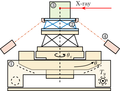
- Compute the wanted pose of the sample with respect to the granite using the micro-station kinematics (Section ref:ssec:nass_ustation_kinematics)
- Measure the sample pose with respect to the granite using the external metrology and internal metrology for Rz (Section ref:ssec:nass_sample_pose_error)
- Compute the sample pose error and map these errors in the frame of the struts (Section ref:ssec:nass_error_struts)
- The complete control architecture is shown in Section ref:ssec:nass_control_architecture
- positioning_error: Explain how the NASS control is made (computation of the wanted position, measurement of the sample position, computation of the errors)
- Schematic with micro-station + nass + metrology + control system => explain what is inside the control system
Micro Station Kinematics
<<ssec:nass_ustation_kinematics>>
- from ref:ssec:ustation_kinematics, computation of the wanted sample pose from the setpoint of each stage.
wanted pose = Tdy * Try * Trz * Tu
Computation of the sample's pose error
<<ssec:nass_sample_pose_error>>
From metrology (here supposed to be perfect 6-DoF), compute the sample's pose error. Has to invert the homogeneous transformation.
In reality, 5DoF metrology => have to estimate the Rz using spindle encoder + nano-hexapod internal metrology (micro-hexapod does not perform Rz rotation).
Position error in the frame of the struts
<<ssec:nass_error_struts>>
Explain how to compute the errors in the frame of the struts (rotating):
- Errors in the granite frame
- Errors in the frame of the nano-hexapod
- Errors in the frame of the struts => used for control
Control Architecture
<<ssec:nass_control_architecture>>
- Say that there are many control strategies. It will be the topic of chapter 2.3. Here, we start with something simple: control in the frame of the struts
\begin{tikzpicture}
  % Blocs
  \node[block={2.0cm}{1.0cm}, fill=colorblue!20!white] (metrology) {Metrology};
  \node[block={2.0cm}{2.0cm}, below=0.1 of metrology, align=center, fill=colorblue!20!white] (nhexa) {Nano\\Hexapod};
  \node[block={3.0cm}{1.5cm}, below=0.1 of nhexa, align=center, fill=colorblue!20!white] (ustation) {Micro\\Station};

  \coordinate[] (inputf)  at ($(nhexa.south west)!0.5!(nhexa.north west)$);
  \coordinate[] (outputfn) at ($(nhexa.south east)!0.3!(nhexa.north east)$);
  \coordinate[] (outputde) at ($(nhexa.south east)!0.7!(nhexa.north east)$);

  \coordinate[] (outputDy) at ($(ustation.south east)!0.1!(ustation.north east)$);
  \coordinate[] (outputRy) at ($(ustation.south east)!0.5!(ustation.north east)$);
  \coordinate[] (outputRz) at ($(ustation.south east)!0.9!(ustation.north east)$);

  \node[block={1.0cm}{1.0cm}, right=0.5 of outputde, fill=colorred!20!white] (Rz_kinematics) {$\bm{J}_{R_z}^{-1}$};
  \node[block={2.0cm}{2.0cm}, right=2.2 of ustation, align=center, fill=colorred!20!white] (ustation_kinematics) {Compute\\Reference\\Position};
  \node[block={2.0cm}{2.0cm}, right=0.8 of ustation_kinematics, align=center, fill=colorred!20!white] (compute_error) {Compute\\Error\\Position};
  \node[block={2.0cm}{2.0cm}, above=0.8 of compute_error, align=center, fill=colorred!20!white] (compute_pos) {Compute\\Sample\\Position};
  \node[block={1.0cm}{1.0cm}, right=0.8 of compute_error, fill=colorred!20!white] (hexa_jacobian) {$\bm{J}$};

  \coordinate[] (inputMetrology) at ($(compute_error.north east)!0.3!(compute_error.north west)$);
  \coordinate[] (inputRz) at ($(compute_error.north east)!0.7!(compute_error.north west)$);

  \node[addb={+}{}{}{}{}, right=0.4 of Rz_kinematics, fill=colorred!20!white] (addRz) {};
  \draw[->] (Rz_kinematics.east) -- (addRz.west);
  \draw[->] (outputRz-|addRz)node[branch]{} -- (addRz.south);

  \draw[->] (outputDy) node[above right]{$r_{D_y}$} -- (outputDy-|ustation_kinematics.west);
  \draw[->] (outputRy) node[above right]{$r_{R_y}$} -- (outputRy-|ustation_kinematics.west);
  \draw[->] (outputRz) node[above right]{$r_{R_z}$} -- (outputRz-|ustation_kinematics.west);

  \draw[->] (metrology.east)node[above right]{$[D_x,\,D_y,\,D_z,\,R_x,\,R_y]$} -- (compute_pos.west|-metrology);
  \draw[->] (addRz.east)node[above right]{$R_z$} -- (compute_pos.west|-addRz);
  \draw[->] (compute_pos.south)node -- (compute_error.north)node[above right]{$\bm{y}_{\mathcal{X}}$};

  \draw[->] (outputde) -- (Rz_kinematics.west) node[above left]{$\bm{\mathcal{L}}$};
  \draw[->] (ustation_kinematics.east) -- (compute_error.west) node[above left]{$\bm{r}_{\mathcal{X}}$};
  \draw[->] (compute_error.east) -- (hexa_jacobian.west) node[above left]{$\bm{\epsilon\mathcal{X}}$};
  \draw[->] (hexa_jacobian.east) -- ++(1.8, 0) node[above left]{$\bm{\epsilon\mathcal{L}}$};

  \draw[->] (outputfn) -- ($(outputfn-|hexa_jacobian.east) + (1.0, 0)$)coordinate(fn) node[above left]{$\bm{f}_n$};

  \begin{scope}[on background layer]
    \node[fit={(metrology.north-|ustation.west) (hexa_jacobian.east|-compute_error.south)}, fill=black!10!white, draw, dashed, inner sep=4pt] (plant) {};
    \node[anchor={north east}] at (plant.north east){$\text{Plant}$};
  \end{scope}

  \node[block, above=0.2 of plant, fill=coloryellow!20!white] (Kiff) {$\bm{K}_{\text{IFF}}$};
  \draw[->] ($(fn)-(0.6,0)$)node[branch]{} |- (Kiff.east);

  \node[addb={+}{}{}{}{}, left=0.8 of inputf] (addf) {};
  \draw[->] (Kiff.west) -| (addf.north);

  \begin{scope}[on background layer]
    \node[fit={(plant.south-|fn) (addf.west|-Kiff.north)}, fill=black!20!white, draw, dashed, inner sep=4pt] (damped_plant) {};
    \node[anchor={north east}] at (damped_plant.north east){$\text{Damped Plant}$};
  \end{scope}

  \begin{scope}[on background layer]
    \node[fit={(metrology.north-|ustation.west) (hexa_jacobian.east|-compute_error.south)}, fill=black!10!white, draw, dashed, inner sep=4pt] (plant) {};
    \node[anchor={north east}] at (plant.north east){$\text{Plant}$};
  \end{scope}

  \node[block, left=0.8 of addf, fill=colorgreen!20!white] (Khac) {$\bm{K}_{\text{HAC}}$};
  \draw[->] ($(hexa_jacobian.east)+(1.4,0)$)node[branch]{} |- ($(Khac.west)+(-0.4, -3.4)$) |- (Khac.west);
  \draw[->] (Khac.east) -- node[midway, above]{$\bm{f}^{\prime}$} (addf.west);
  \draw[->] (addf.east) -- (inputf) node[above left]{$\bm{f}$};
\end{tikzpicture}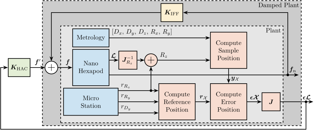
Decentralized Active Damping
<<sec:nass_active_damping>>
Introduction ignore
- How to apply/optimize IFF on an hexapod?
- Robustness to payload mass
- Root Locus
- Damping optimization
Explain which samples are tested:
- 1kg, 25kg, 50kg
- cylindrical, 200mm height?
- control_active_damping
- active damping for stewart platforms
- Vibration Control and Active Damping
IFF Plant
- Show how it changes with the payload mass (1, 25, 50)
- Effect of rotation (no rotation - 60rpm)
- Added parallel stiffness
%% Identify the plant dynamics using the Simscape model

% Initialize each Simscape model elements
initializeGround();
initializeGranite();
initializeTy();
initializeRy();
initializeRz();
initializeMicroHexapod();
initializeSimplifiedNanoHexapod();
initializeSample('type', 'cylindrical');

initializeSimscapeConfiguration('gravity', false);
initializeDisturbances('enable', false);
initializeLoggingConfiguration('log', 'none');
initializeController('type', 'open-loop');
initializeReferences();

% Input/Output definition
% clear io; io_i = 1;
% io(io_i) = linio([mdl, '/Controller'],     1, 'openinput');             io_i = io_i + 1; % Actuator Inputs [V]
% io(io_i) = linio([mdl, '/Micro-Station'],  3, 'openoutput', [], 'Vs');  io_i = io_i + 1; % Force Sensors voltages [V]
% io(io_i) = linio([mdl, '/Tracking Error'], 1, 'openoutput', [], 'EdL'); io_i = io_i + 1; % Position Errors [m]

% % With no payload
% Gm = exp(-1e-4*s)*linearize(mdl, io);
% Gm.InputName  = {'u1', 'u2', 'u3', 'u4', 'u5', 'u6'};
% Gm.OutputName = {'Vs1', 'Vs2', 'Vs3', 'Vs4', 'Vs5', 'Vs6', ...
%                  'eL1', 'eL2', 'eL3', 'eL4', 'eL5', 'eL6'};
Controller Design
- Use Integral controller (with parallel stiffness)
- Show Root Locus (show that without parallel stiffness => unstable?)
- Choose optimal gain. Here in MIMO, cannot have optimal damping for all modes. (there is a paper that tries to optimize that)
- Show robustness to change of payload (loci?) / Change of rotating velocity ?
- Reference to paper showing stability in MIMO for decentralized IFF
Sensitivity to disturbances
Disturbances:
- floor motion
- Spindle X and Z
- Direct forces?
- Compute sensitivity to disturbances with and without IFF (and compare without the NASS)
- Maybe noise budgeting, but may be complex in MIMO… ?
Centralized Active Vibration Control
<<sec:nass_hac>>
Introduction ignore
- uncertainty_experiment: Effect of experimental conditions on the plant (payload mass, Ry position, Rz position, Rz velocity, etc…)
- Effect of micro-station compliance
- Effect of IFF
- Effect of payload mass
- Decoupled plant
- Controller design
From control kinematics:
- Talk about issue of not estimating Rz from external metrology? (maybe could be nice to discuss that during the experiments!)
- Show what happens is Rz is not estimated (for instance supposed equaled to zero => increased coupling)
HAC Plant
- Compute transfer function from $\bm{f}$ to $\bm{\epsilon\mathcal{L}}$ (with IFF applied) for all masses
- Show effect of rotation
- Show effect of payload mass
- Compare with undamped plants
Controller design
- Show design HAC with formulas and parameters
- Show robustness with Loci for all masses
Sensitivity to disturbances
- Compute transfer functions from spindle vertical error to sample vertical error with HAC-IFF Compare without the NASS, and with just IFF
- Same for horizontal
Tomography experiment
- With HAC-IFF, perform tomography experiment, and compare with open-loop
- Take into account disturbances, metrology sensor noise. Maybe say here that we don't take in account other noise sources as they will be optimized latter (detail design phase)
- Tomography + lateral scans (same as what was done in open loop here)
- Validation of concept
Conclusion
<<sec:nass_conclusion>>