131 KiB
Nano Active Stabilization System - Introduction
- Context of this thesis
- Challenge definition
- Literature Review
- Original Contributions
- Introduction
- Active Damping of rotating mechanical systems using Integral Force Feedback
- Design of complementary filters using $\mathcal{H}_\infty$ Synthesis and sensor fusion
- Multi-body simulations with reduced order flexible bodies obtained by FEA
- Robustness by design
- Mechatronics design
- 6DoF vibration control of a rotating platform
- Experimental validation of the Nano Active Stabilization System
- Thesis Outline - Mechatronics Design Approach
- Bibliography
- Footnotes
Context of this thesis
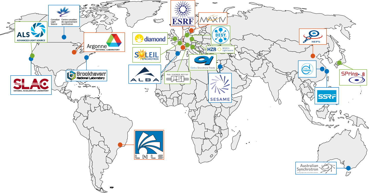
Synchrotron Radiation Facilities
Accelerating electrons to produce intense X-ray
- Explain what is a Synchrotron: light source
- Say how many there are in the world (~50). The main ones are shown in Figure ref:fig:introduction_synchrotrons.
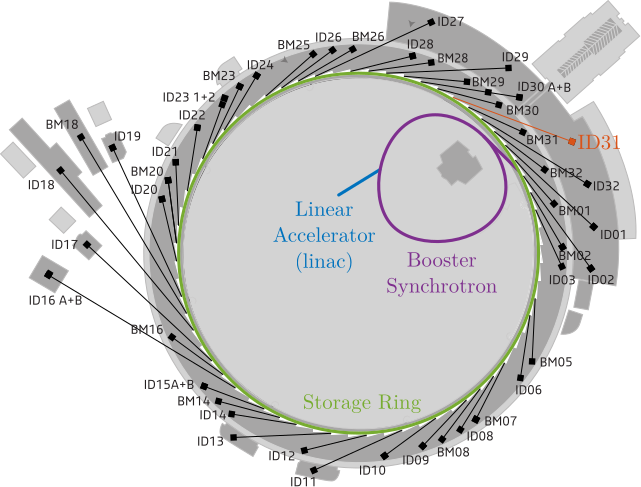
- Electron part: LINAC, Booster, Storage Ring ref:fig:introduction_esrf_schematic
- Synchrotron radiation: Insertion device / Bending magnet
- Many beamlines (large diversity in terms of instrumentation and science)
-
Science that can be performed:
- structural biology, structure of materials, matter at extreme, …
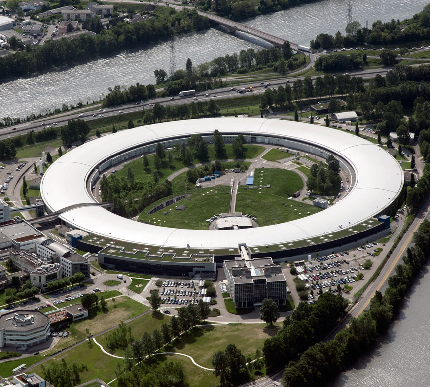
The European Synchrotron Radiation Facility
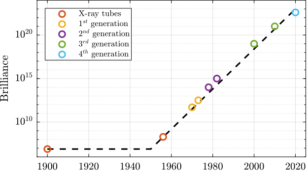
3rd and 4th generation Synchrotrons
Brilliance: figure of merit for synchrotron
- 4th generation light sources cite:&raimondi21_commis_hybrid_multib_achrom_lattic
The ID31 ESRF Beamline
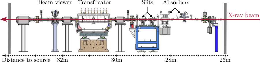
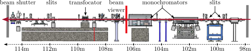
Beamline Layout
- General layout: source (insertion device), optical hutches (OH1, OH2), experimental hutch (EH)
- Beamline layout (OH Figure ref:fig:introduction_id31_oh, EH ref:fig:introduction_id31_cad) All these optical instruments are used to "shape" the x-ray beam as wanted (monochromatic, wanted size, focused, etc…)
- ID31 and Micro Station (Figure ref:fig:introduction_id31_cad) Check https://www.esrf.fr/UsersAndScience/Experiments/StructMaterials/ID31 https://www.wayforlight.eu/beamline/23244
- X-ray beam + detectors + sample stage
- Focusing optics
- Optical schematic with: source, lens, sample and detector. Explain that what is the most important is the relative position between the sample and the lens.
- Explain the XYZ frame for all the thesis (ESRF convention: X: x-ray, Z gravity up)
\bigskip
\begin{tikzpicture}
  \node[inner sep=0pt, anchor=south west] (photo) at (0,0)
  {\includegraphics[width=0.39\textwidth]{/home/thomas/Cloud/documents/reports/phd-thesis/figs/exp_setup_photo.png}};

  \coordinate[] (aheight) at (photo.north west);
  \coordinate[] (awidth)  at (photo.south east);

  \coordinate[] (granite) at ($0.1*(aheight)+0.1*(awidth)$);
  \coordinate[] (trans)   at ($0.5*(aheight)+0.4*(awidth)$);
  \coordinate[] (tilt)    at ($0.65*(aheight)+0.75*(awidth)$);
  \coordinate[] (hexapod) at ($0.7*(aheight)+0.5*(awidth)$);
  \coordinate[] (sample)  at ($0.9*(aheight)+0.55*(awidth)$);

  % Granite
  \node[labelc] at (granite) {1};
  % Translation stage
  \node[labelc] at (trans) {2};
  % Tilt Stage
  \node[labelc] at (tilt) {3};
  % Micro-Hexapod
  \node[labelc] at (hexapod) {4};
  % Sample
  \node[labelc] at (sample) {5};

  % Axis
  \begin{scope}[shift={($0.07*(aheight)+0.87*(awidth)$)}]
    \draw[->] (0, 0) -- ++(55:0.7) node[above] {$y$};
    \draw[->] (0, 0) -- ++(90:0.9) node[left] {$z$};
    \draw[->] (0, 0) -- ++(-20:0.7) node[above] {$x$};
  \end{scope}
\end{tikzpicture}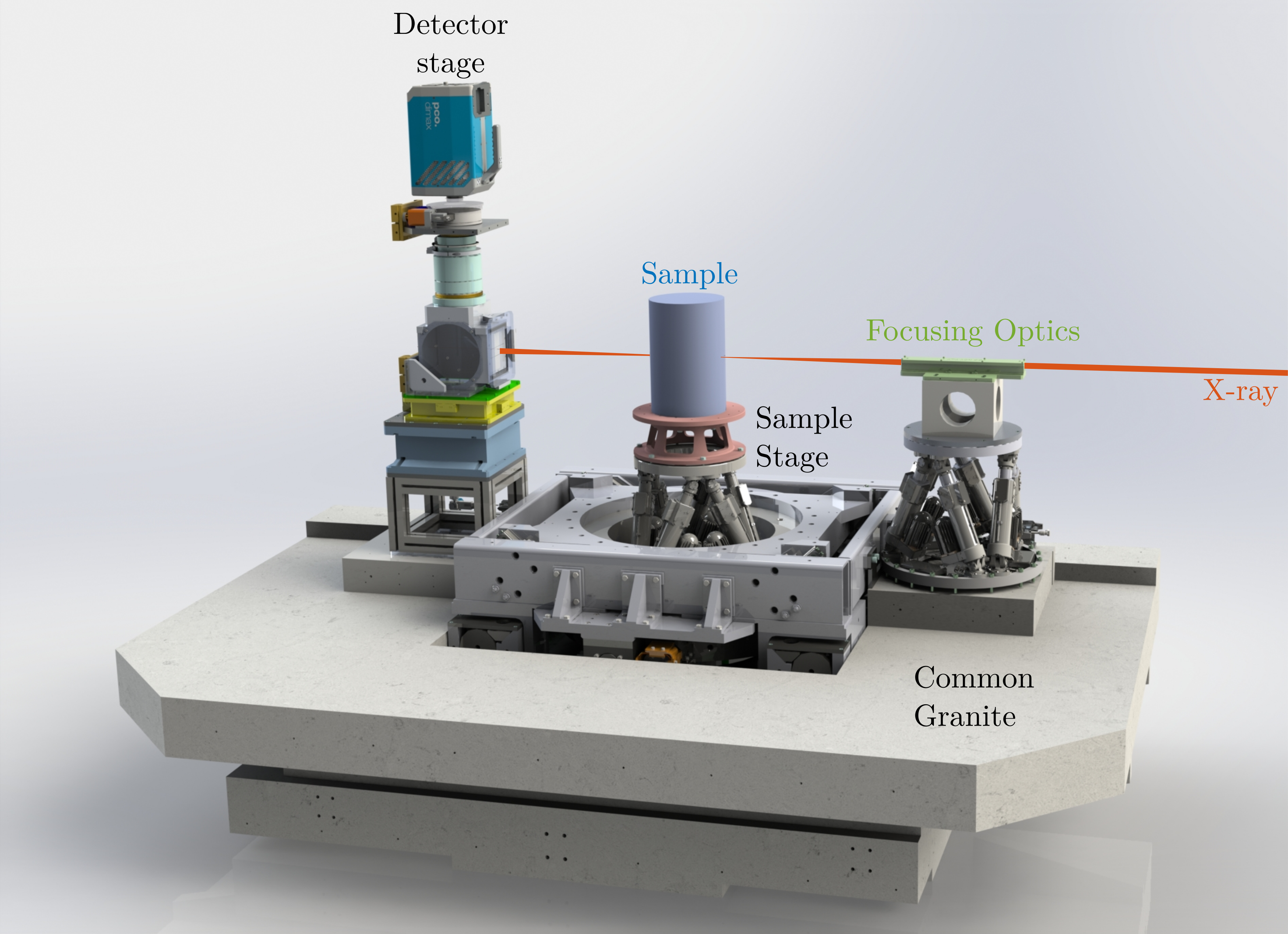
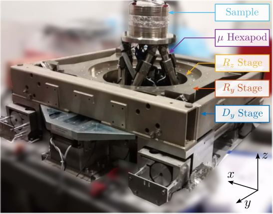
Positioning End Station: The Micro-Station
Micro-Station:
- DoF with strokes: Ty, Ry, Rz, Hexapod
- Experiments: tomography, reflectivity, truncation rod, … Make a table to explain the different "experiments"
- Explain how it is used (positioning, scans), what it does. But not about the performances
- Different sample environments
Scientific experiments performed on ID31
- Few words about science made on ID31 and why nano-meter accuracy is required
-
Typical experiments (tomography, …), various samples (up to 50kg), sample environments (high temp, cryo, etc..)
- Alignment of the sample, then
- Reflectivity
- Tomography
- Diffraction tomography: most critical
-
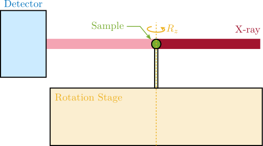
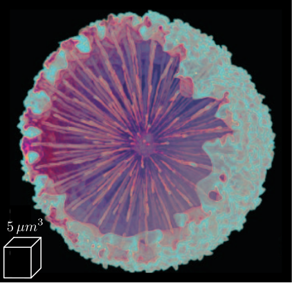
Two example:
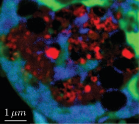
- Tomography: compute image as a function of the angle. To reconstruct 3D image, the position has to be known with good accuracy cite:&schoeppler17_shapin_highl_regul_glass_archit
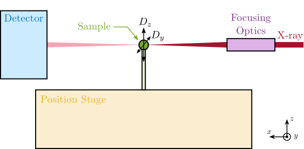
- Mapping: focused beam on the sample, 20nm step size, accuracy of the obtained image is directly linked to the beam size and the position accuracy/vibrations cite:&sanchez-cano17_synch_x_ray_fluor_nanop
Need of Accurate Positioning End-Stations with High Dynamics
A push towards brighter and smaller beams
Improvement of both the light source and the instrumentation:
- EBS: smaller source + higher flux ref:fig:introduction_beam_3rd_4th_gen
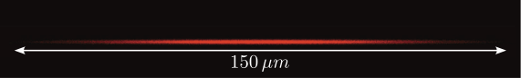
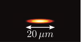
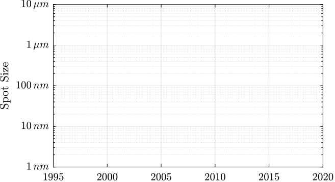
- ESRF Red Book (1987): very few beamline projects aiming even for 10 micron sized beams Now optics exist for 10nm beams
- Better focusing optic (add some links): beam size in the order of 10 to 20nm FWHM (reference) ref:fig:introduction_moore_law_focus crossed silicon compound refractive lenses, KB mirrors [17], zone plates [18], or multilayer Laue lenses [19] cite:&barrett16_reflec_optic_hard_x_ray
Higher flux density (+high energy of the ID31 beamline) => Radiation damage: needs to scan the sample quite fast with respect to the focused beam
- Allowed by better detectors: higher sampling rates and lower noise => possible to scan fast cite:&hatsui15_x_ray_imagin_detec_synch_xfel_sourc
New dynamical positioning needs
"from traditional step by step scans to fly-scan"
Fast scans + needs of high accuracy and stability => need mechatronics system with:
- accurate metrology
- multi degree of freedom positioning systems
- fast feedback loops
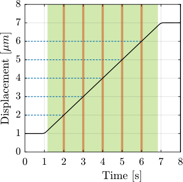
Shift from step by step scan to fly-scan cite:huang15_fly_scan_ptych
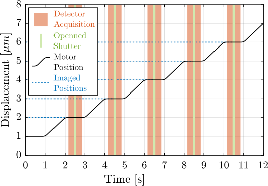
- Much lower pixel size + large image => takes of lot of time if captured step by step. Explain what is step by step scanning: move motors from point A to point B, stops, start detector acquisition, open shutter , close the shutter, move to point C, …
In traditional step scan mode, each exposure position requires the system to stop prior to data acquisition, which may become a limiting factor when fast data collection is required. Fly-scanning is chosen as a preferred solution that helps overcome such speed limitations [5, 6]. In fly-scan mode, the sample keeps moving and a triggering system generates trigger signals based on the position of the sample or the time elapsed. The trigger signals are used to control detector exposure.
Subject of this thesis: design of high performance positioning station with high dynamics and nanometer accuracy
Nano Positioning End-Stations
End-Station with Stacked Stages
Stacked stages:
- errors are combined
To have acceptable performances / stability:
- limited number of stages
- high performances stages (air bearing etc…)
Examples:
- ID01 cite:&leake19_nanod_beaml_id01
- ID11 cite:&wright20_new_oppor_at_mater_scien
- ID13 cite:&riekel10_progr_micro_nano_diffr_at
Explain limitations => Thermal drifts, run-out errors of spindles (improved by using air bearing), straightness of translation stages, …
Online Metrology
The idea of having an external metrology to correct for errors is not new.
Several strategies:
- only used for measurements (post processing)
- for calibration
- for triggering detectors
- for real time positioning control (Figure ref:fig:introduction_active_stations)
Sensors:
- Capacitive: cite:&schroer17_ptynam;&villar18_nanop_esrf_id16a_nano_imagin_beaml;&schropp20_ptynam
-
Fiber Interferometers Interferometers:
- Attocube FPS3010 Fabry-Pérot interferometers: cite:&nazaretski15_pushin_limit;&stankevic17_inter_charac_rotat_stages_x_ray_nanot;&engblom18_nanop_resul;&nazaretski22_new_kirkp_baez_based_scann
- Attocube IDS3010 Fabry-Pérot interferometers: cite:&holler17_omny_pin_versat_sampl_holder;&holler18_omny_tomog_nano_cryo_stage;&kelly22_delta_robot_long_travel_nano
- PicoScale SmarAct Michelson interferometers: cite:&schroer17_ptynam;&schropp20_ptynam;&xu23_high_nsls_ii;&geraldes23_sapot_carnaub_sirius_lnls


| Architecture | Metrology | Usage | Institute | References |
|---|---|---|---|---|
| Sample | 3 Capacitive | Post processing | NSLS | cite:&wang12_autom_marker_full_field_hard |
| XYZ Stage | $D_yD_zR_x$ | (X8C) | Figure ref:fig:introduction_stages_wang | |
| Metrology Ring | ||||
| Spindle | ||||
| Ball-lens retroreflector / Sample | 3 interferometers | Characterization | PETRA III | cite:&schroer17_ptynam;&schropp20_ptynam |
| XYZ piezo stage ($100\,\mu m$) | $D_yD_z$ | (P06) | Figure ref:fig:introduction_stages_schroer | |
| Spindle ($180\,\text{deg}$) | ||||
| Metrology Ring / Sample | 2 interferometers | Detector | NSLS | cite:&xu23_high_nsls_ii |
| Spindle | $D_yD_z$ | triggering | (HRX) | |
| XYZ piezo stage |
Active Control of Positioning Errors
For some applications (especially when using a nano-beam), the position has not only to be measured, but to be controlled.
Actuators:
- Piezoelectric: cite:&nazaretski15_pushin_limit;&holler17_omny_pin_versat_sampl_holder;&holler18_omny_tomog_nano_cryo_stage;&villar18_nanop_esrf_id16a_nano_imagin_beaml;&nazaretski22_new_kirkp_baez_based_scann
- 3-phase linear motor: cite:&stankevic17_inter_charac_rotat_stages_x_ray_nanot;&engblom18_nanop_resul
- Voice Coil: cite:&kelly22_delta_robot_long_travel_nano;&geraldes23_sapot_carnaub_sirius_lnls
Bandwidth: rarely specificity. Usually slow, so that only drifts are compensated. Only recently, high bandwidth (100Hz) have been reported with the use of voice coil actuators cite:&kelly22_delta_robot_long_travel_nano;&geraldes23_sapot_carnaub_sirius_lnls.
Full rotation for tomography:
- Spindle above XYZ stage: cite:&stankevic17_inter_charac_rotat_stages_x_ray_nanot;&holler17_omny_pin_versat_sampl_holder;&holler18_omny_tomog_nano_cryo_stage;&villar18_nanop_esrf_id16a_nano_imagin_beaml;&engblom18_nanop_resul;&nazaretski22_new_kirkp_baez_based_scann;&xu23_high_nsls_ii
- Spindle bellow XYZ stage: cite:&wang12_autom_marker_full_field_hard;&schroer17_ptynam;&schropp20_ptynam;&geraldes23_sapot_carnaub_sirius_lnls
Only for mapping: cite:&nazaretski15_pushin_limit;&kelly22_delta_robot_long_travel_nano


Payload capabilities:
- All are only supported calibrated, micron scale samples
- Higher sample masses to up to 500g have been reported in cite:&nazaretski22_new_kirkp_baez_based_scann;&kelly22_delta_robot_long_travel_nano
100 times heavier payload capabilities than previous stations with similar performances.
| Architecture | Metrology | Stroke | Bandwidth | Institute | References |
|---|---|---|---|---|---|
| Mirror / Sample | 3 Interferometers | n/a | APS | cite:&nazaretski15_pushin_limit | |
| XYZ piezo motors | $D_xD_yD_z$ | $D_xD_yD_z: 3\,\text{mm}$ | Figure ref:fig:introduction_stages_nazaretski | ||
| Metrology Ring / Sample | 12 Capacitive | light | 10 Hz | ESRF | cite:&villar18_nanop_esrf_id16a_nano_imagin_beaml |
| Spindle | $D_xD_yD_zR_xR_y$ | $R_z: 180\,\text{deg}$ | (ID16a) | Figure ref:fig:introduction_stages_villar | |
| Piezo Hexapod | $D_xD_yD_z: 50\,\mu m$ | ||||
| $R_x R_y: 500\,\mu \text{rad}$ | |||||
| Spherical Reference / Sample | 5 Interferometers | light | n/a | PSI | cite:&holler17_omny_pin_versat_sampl_holder;&holler18_omny_tomog_nano_cryo_stage |
| Spindle | $D_yD_zR_x$ | $R_z: 365\,\text{deg}$ | (OMNY) | ||
| Piezo Tripod | $D_xD_yD_z: 400\,\mu m$ | ||||
| Cylindrical Reference / Sample | 5 Interferometers | light | n/a | Soleil | cite:&stankevic17_inter_charac_rotat_stages_x_ray_nanot;&engblom18_nanop_resul |
| Spindle | $D_xD_yD_zR_xR_y$ | $R_z: 360\,\text{deg}$ | |||
| Stacked XYZ linear motors | $D_xD_yD_z: 400\,\mu m$ | ||||
| Metrology Ring / Sample | 3 Interferometers | up to 500g | n/a | NSLS | cite:&nazaretski22_new_kirkp_baez_based_scann |
| Spindle | $D_xD_yD_z$ | $R_z: 360\,\text{deg}$ | (SRX) | ||
| XYZ piezo | $D_xD_yD_z: 100\,\mu m$ | ||||
| Mirrors / Sample | 3 Interferometers | up to 350g | 100 Hz | Diamond | cite:&kelly22_delta_robot_long_travel_nano |
| Parallel XYZ voice coil | $D_xD_yD_z$ | $D_xD_yD_z: 3\,\text{mm}$ | (I14) | ||
| Retroreflectors / Samples | 3 Interferometers | light | 100 Hz | LNLS | cite:&geraldes23_sapot_carnaub_sirius_lnls |
| Parallel XYZ voice coil | $D_xD_yD_z$ | $D_yD_z: 3\,\text{mm}$ | (Carnauba) | ||
| Spindle | $R_z: \pm 110\,\text{deg}$ | ||||
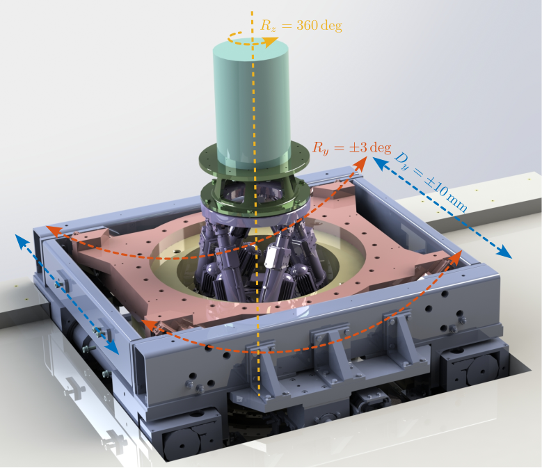
| Sample | 6 Interferometers | up to 50kg | ESRF | cite:&dehaeze18_sampl_stabil_for_tomog_exper;&dehaeze21_mechat_approac_devel_nano_activ_stabil_system | |
| Hexapod | $D_xD_yD_zR_xR_y$ | (ID31) | Figure ref:fig:introduction_nass_concept_schematic | ||
| Spindle | $R_z : 360\,\text{deg}$ | ||||
| Ry | $R_y : \pm 3\,\text{deg}$ | ||||
| Ty | $D_y : \pm 5\,\text{mm}$ |
Long Stroke - Short Stroke architecture
Speak about two stage control?
- Long stroke + short stroke
- Usually applied to 1dof, 3dof (show some examples: disk drive, wafer scanner)
- Any application in 6DoF? Maybe new!
- In the table, say which ones are long stroke / short stroke. Some new stages are just long stroke (voice coil)


Challenge definition
Multi degrees of freedom, long stroke and highly accurate positioning end station
Performance limitation of "stacked-stages" end-stations
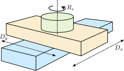
Typical positioning end station (Figure ref:fig:introduction_translation_stage):
- stacked stages
- Ball-screw, linear guides, rotary motor
Explain the limitation of performances:
- Backlash, play, thermal expansion, guiding imperfections, …
- Give some numbers: straightness of the Ty stage for instance, change of $0.1^oC$ with steel gives x nm of motion
- Vibrations
- Possibility to have linear/rotary encoders that correct the motion in the considered DoF, but does not change anything to the other 5DoF

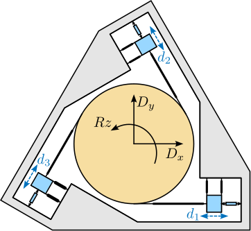
Flexure based positioning stations may give better positioning requirements, but are limited to short stroke. Advantages: no backlash, etc… But: limited to short stroke Picture of schematic of one positioning station based on flexure
Explain example of Figure ref:fig:introduction_flexure_stage.

Combining, long stroke and accuracy in multi-DoF is challenging.
Positioning accuracy of the ID31 Micro-Station
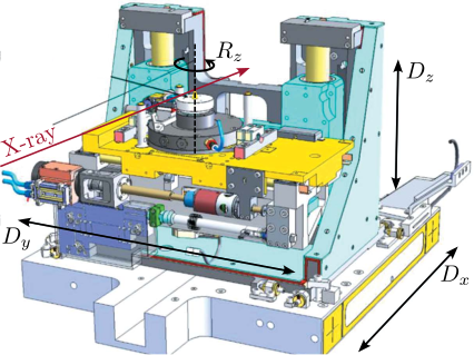
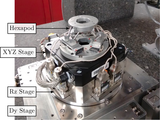
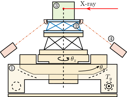
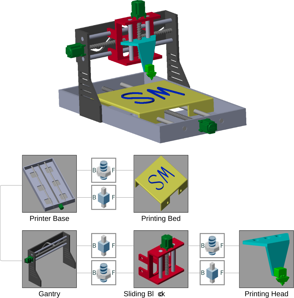
Presentation of the Micro-Station in details ref:fig:introduction_micro_station:
- Goal of each stage (e.g. micro-hexapod: static positioning, Ty and Rz: scans, …)
- Stroke
- Initial design objectives: as stiff as possible, smallest errors as possible
Explain that this micro-station can only have ~10um / 10urad of accuracy due to physical limitation.
New positioning requirements
- To benefits from nano-focusing optics, new source, etc… new positioning requirements
-
Positioning requirements on ID31:
- Maybe make a table with the requirements and the associated performances of the micro-station
- Make tables with the wanted motion, stroke, accuracy in different DoF, etc..
- Sample masses
The goal in this thesis is to increase the positioning accuracy of the micro-station to fulfil the initial positioning requirements.
Goal: Improve accuracy of 6DoF long stroke position platform
The Nano Active Stabilization System
NASS Concept
In order to address the new positioning requirements, the concept of…
Briefly describe the NASS concept. 6DoF vibration control platform on top of a complex positioning platform that correct positioning errors based on an external metrology
It is composed of mainly four elements:
- The micro station
- A 5 degrees of freedom metrology system
- A 5 or 6 degrees of freedom stabilization platform
- Control system and associated instrumentation
Online Metrology system
The accuracy of the NASS will only depend on the accuracy of the metrology system.
Requirements:
- 5 DoF
- long stroke
- nano-meter accurate
- high bandwidth
Concept:
- Fiber interferometers
- Spherical reflector with flat bottom
- Tracking system (tip-tilt mechanism) to keep the beam perpendicular to the mirror surface: Spherical mirror with center at the point of interest => No Abbe errors
- XYZ positions from at least 3 interferometers pointing at the spherical surface
- Rx/Ry angles from at least 3 interferometers pointing at the bottom flat surface
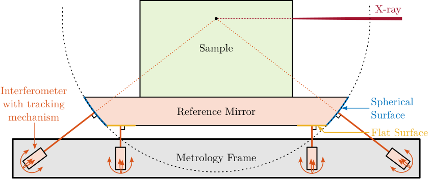
Complex mechatronics system on its own. This metrology system is not further discussed in this thesis as it is still under active development. In the following of this thesis, it is supposed that the metrology system is accurate, etc..
Active Stabilization Platform
- 5 DoF
- High dynamics
- Nano-meter capable (no backlash)
- Accept payloads up to 50kg
MIMO robust control strategies
Explain the robustness need?
- 24 7/7 …
- That is why most of end-stations are based on well-proven design (stepper motors, linear guides, ball bearing, …)
- Plant uncertainty: many different samples, use cases, rotating velocities, etc…
Trade-off between robustness and performance in the design of feedback system.
Predictive Design
-
The performances of the system will depend on many factors:
- sensors
- actuators
- mechanical design
- achievable bandwidth
- Need to evaluate the different concepts, and predict the performances to guide the design
- The goal is to design, built and test this system such that it work as expected the first time. Very costly system, so must be correct.
-
Challenge:
- proper design methodology
- accurate models
Control Challenge
High bandwidth, 6 DoF system for vibration control, fixed on top of a complex multi DoF positioning station, robust, …
- Many different configurations (tomography, Ty scans, slow fast, …)
- Complex MIMO system. Dynamics of the system could be coupled to the complex dynamics of the micro station
- Rotation aspect, gyroscopic effects, actuators are rotating with respect to the sensors
- Robustness to payload change: very critical. Say that high performance systems (lithography machines, etc…) works with calibrated payloads. Being robust to change of payload inertia means large stability margins and therefore less performance.
[A] Literature Review
Maybe remove this section has it seems it is discussed elsewhere?
Multi-DoF dynamical positioning stations
Serial and Parallel Kinematics
Example of several dynamical stations:
- XYZ piezo stages
- Delta robot? Octoglide?
- Stewart platform
Serial vs parallel kinematics (table?)
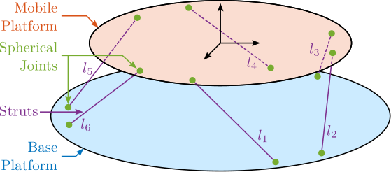
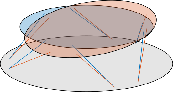
Stewart platforms
- Explain the normal stewart platform architecture
- Make a table that compares the different stewart platforms for vibration control. Geometry (cubic), Actuator (soft, stiff), Sensor, Flexible joints, etc.
Mechatronics approach
Predicting performances using models
cite:&monkhorst04_dynam_error_budget
Can use several models:
- Lumped mass-spring-damper models
- usually uniaxial, easily put into equations, 1dof per considered mass cite:rankers98_machin
- Multi-Body Models
- usually 6dof per considered solid body, some may be constrained using joints
- Finite element models
- Can include FEM into multi-body models: Sub structuring (cite:&brumund21_multib_simul_reduc_order_flexib_bodies_fea)
\begin{tikzpicture}
  % ====================
  % Parameters
  % ====================
  \def\massw{2.2}  % Width of the masses
  \def\massh{0.8}  % Height of the masses
  \def\spaceh{1.2} % Height of the springs/dampers
  \def\dispw{0.4}  % Width of the dashed line for the displacement
  \def\disph{0.4}  % Height of the arrow for the displacements
  \def\bracs{0.05} % Brace spacing vertically
  \def\brach{-12pt} % Brace shift horizontaly
  \def\fsensh{0.2} % Height of the force sensor
  \def\velsize{0.2} % Size of the velocity sensor
  % ====================


  % ====================
  % Floor
  % ====================
  \draw (-0.5*\massw, 0) -- (0.5*\massw, 0);
  % \draw[dashed] (0.5*\massw, 0) -- ++(\dispw, 0);
  % \draw[->, draw=colorred] (0.5*\massw+0.5*\dispw, 0) -- ++(0, \disph) node[right, color=colorred]{$x_{f}$};
  % ====================

  % ====================
  % Granite
  \begin{scope}[shift={(0, 0)}]
    % Mass
    \draw[fill=white] (-0.5*\massw, \spaceh) rectangle (0.5*\massw, \spaceh+\massh) node[pos=0.5]{$m_{1}$};

    % Spring, Damper, and Actuator
    \draw[spring] (-0.3*\massw, 0) -- (-0.3*\massw, \spaceh) node[midway, left=0.1]{$k_{1}$};
    \draw[damper] ( 0.3*\massw, 0) -- ( 0.3*\massw, \spaceh) node[midway, left=0.2]{$c_{1}$};

    % Displacement
    \draw[dashed] (0.5*\massw, \spaceh+\massh) -- ++(\dispw, 0);
    \draw[->] (0.5*\massw+0.5*\dispw, \spaceh+\massh) -- ++(0, \disph) node[right]{$x_{1}$};
  \end{scope}
  % ====================


  % ====================
  % Stages
  \begin{scope}[shift={(0, \spaceh+\massh)}]
    % Mass
    \draw[fill=white] (-0.5*\massw, \spaceh) rectangle (0.5*\massw, \spaceh+\massh) node[pos=0.5]{$m_{2}$};

    % Spring, Damper, and Actuator
    \draw[spring] (-0.4*\massw, 0) -- (-0.4*\massw, \spaceh) node[midway, left=0.1]{$k_{1}$};
    \draw[damper] (0,           0) -- ( 0,          \spaceh) node[midway, left=0.2]{$c_{2}$};
    \draw[actuator={0.45}{0.2}{black}] ( 0.4*\massw, 0) -- (0.4*\massw, \spaceh) node[midway, left=0.1]{$F$};

    % Displacement
    \draw[dashed] (0.5*\massw, \spaceh+\massh) -- ++(\dispw, 0);
    \draw[->] (0.5*\massw+0.5*\dispw, \spaceh+\massh) -- ++(0, \disph) node[right]{$x_{2}$};
  \end{scope}
  % ====================
\end{tikzpicture}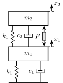
Closed-Loop Simulations
cite:&schmidt20_desig_high_perfor_mechat_third_revis_edition
Once a model of the system is obtained: develop controller based on linearized model.
\begin{tikzpicture}
  \node[block] (controller) {Controller};
  \node[block, right = 1 of controller] (driver) {Driver};
  \node[block, right = 1 of driver] (actuator) {Actuator};
  \node[block, right = 1 of actuator, align=center] (system) {Mechanical\\System};
  \node[block, right = 1 of system] (sensor) {Sensor};

  % Connections and labels
  \draw[->] (controller.east) node[above right]{$u$} -- (driver.west);
  \draw[->] (driver.east) -- (actuator.west);
  \draw[->] (actuator.east) -- (system.west);
  \draw[->] (system.east) --node[midway, above]{$y$} (sensor.west);
  \draw[->] (sensor.east) -- ++(1.2, 0);
  \draw[->] ($(sensor.east)+(0.6,0)$)node[branch]{}node[above]{$y_m$} -- ++(0, -2.0) -| (controller.south);

  \draw[<-] (controller.west) -- ++(-1.0, 0) node[above right]{$r$};
  \draw[<-] (driver.north)   -- ++(0, 1.2) node[below right, align=left]{$d_u$};
  \draw[<-] (system.north)   -- ++(0, 1.2) node[below right, align=left]{$d_y$};
  \draw[<-] (sensor.north)   -- ++(0, 1.2) node[below right, align=left](sensornoise){$n$};

  % Plant
  \begin{scope}[on background layer]
    \node[fit={(driver.south west) (sensornoise.north -| sensor.east)}, fill=black!20!white, draw, dashed, inner sep=8pt] (plant) {};
    \node[below] at (plant.north) {\textbf{Plant}};
  \end{scope}

  \draw[->, dashed] ($(plant.south) + (0, -0.3)$) arc (90:-90:0.3) -- ++(-2.5, 0) arc (-90:-270:0.3);
  \node[left] at ($(plant.south) + (0, -0.6)$) {Feedback Loop}
\end{tikzpicture}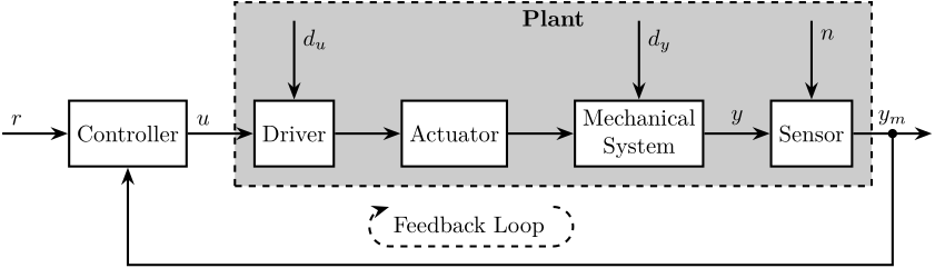
Say what can limit the performances for a complex mechatronics systems as this one:
- Disturbances affecting the plant output $d_y$
- Measurement noise $n$
- DAC / amplifier noise (actuator) $d_u$
- Feedback system / bandwidth
- $r$, $y_m$
Simulations can help evaluate the behavior of the system.
Dynamic Error Budgeting
cite:&monkhorst04_dynam_error_budget
cite:jabben07_mechat
cite:&okyay16_mechat_desig_dynam_contr_metrol
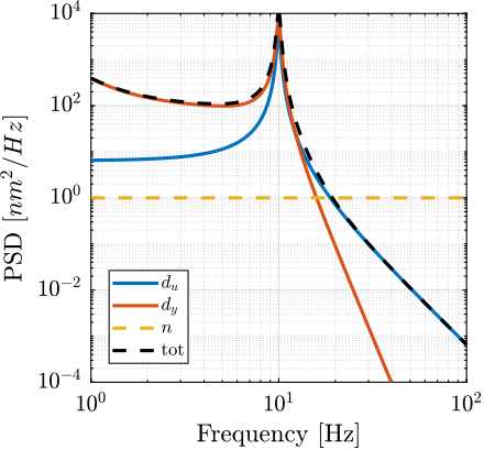
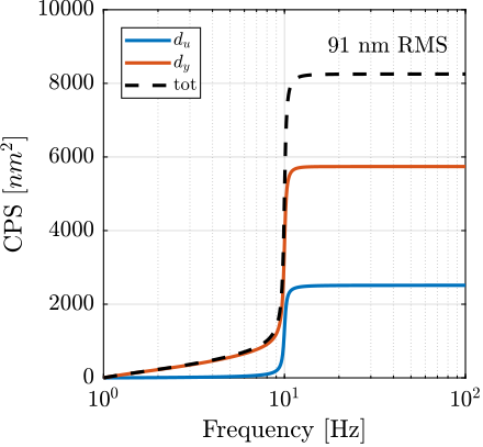
- "the disturbance signals are modeled with their power spectral density (PSD), assuming that they are stationary stochastic processes which are not correlated with each other"
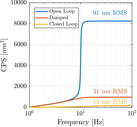
- Effects of $d_u$, $d_y$ and $n$ on $y$ can be estimated from their PSD and the closed-loop transfer functions This gives a first idea of the limiting factor as a function of frequency. In order to determine whether each disturbance/noise impact the performances, cumulative power spectrum can be used: this gives the RMS value Then, this help to know the different actions to improve the performances: reduce sensor noise or driver electrical noise, work on reducing disturbances like damping resonances, increase feedback bandwidth, …)
Stewart platforms: Control architecture
Introduction ignore
Different control goals:
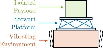
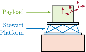
- Vibration Isolation ref:fig:introduction_stewart_isolation
- Position ref:fig:introduction_stewart_positioning
Depending on the goal, different sensors and different architectures.
For the NASS, both objectives.
Active Damping and Vibration Control
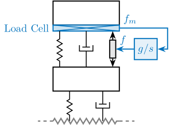
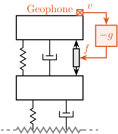
Two main active vibration isolation strategies cite:&collette11_review_activ_vibrat_isolat_strat:
- IFF using collocated force sensors / load cell cite:&chesne16_enhan_dampin_flexib_struc_using_force_feedb
- Skyhook damping using inertial sensors (accelerometers, geophones), usually in the frame of the struts
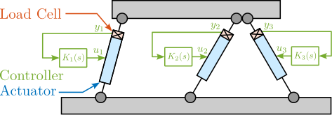
Usually, "decentralized", in the frame of the struts (Figure ref:fig:introduction_control_decentralized). Optimization based on one "strut", and then applied to all the struts simultaneously to obtained a 6-DoF active damping / vibration control system.
If narrow band disturbances: Adaptive feedforward control.
Position and Pointing Control
Control based on position sensors. Wanted position is generally expressed in the cartesian frame.
Sensors can be:
- In the frame of the struts (LVDT, Encoder, Strain gauges): usually decentralized control (Figure ref:fig:introduction_control_decentralized_diagram)
- External sensors: centralized
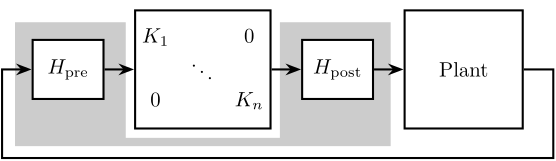
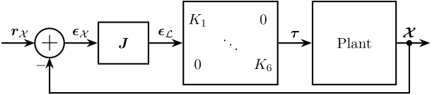
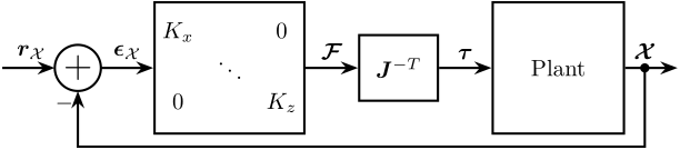
When using external sensors, a decoupling strategy is usually employed (Figure ref:fig:introduction_control_decoupling):
- Jacobian matrices: frame of the struts or cartesian frame
- Modal control
- Singular Value Decomposition
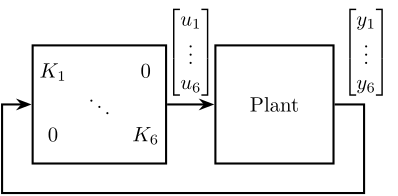
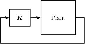
- Multivariable control: LQG, H-Infinity (Figure ref:fig:introduction_control_mimo)
From cite:&thayer02_six_axis_vibrat_isolat_system:
Experimental closed-loop control results using the hexapod have shown that controllers designed using a decentralized single-strut design work well when compared to full multivariable methodologies.
- Explain the Jacobian matrix
When decoupling using the Jacobian matrix, the control can be performed in the frame of the struts (Figure ref:fig:introduction_control_centralized_struts) or in the cartesian frame (Figure ref:fig:introduction_control_centralized_cartesian).
\bigskip
Use of Multiple Sensors
Often, both vibration control and position control is wanted. In that case, the use of multiple sensors can lead to improved performances.
Sensors:
- collocated force (load cell) sensors
- collocated accelerometer
- displacement (eddy current)
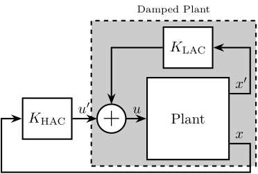
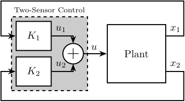
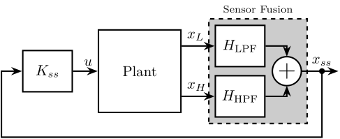
Several strategies can be employed:
- HAC-LAC cite:geng95_intel_contr_system_multip_degree,wang16_inves_activ_vibrat_isolat_stewar,li01_simul_vibrat_isolat_point_contr,pu11_six_degree_of_freed_activ,xie17_model_contr_hybrid_passiv_activ
- Sensor Fusion cite:tjepkema12_activ_ph,tjepkema12_sensor_fusion_activ_vibrat_isolat_precis_equip,hauge04_sensor_contr_space_based_six
- Two Sensor control: cite:hauge04_sensor_contr_space_based_six,tjepkema12_activ_ph
Comparison between "two sensor control" and "sensor fusion" is given in cite:&beijen14_two_sensor_contr_activ_vibrat.
\bigskip
Original Contributions
Introduction ignore
This thesis proposes several contributions in the fields of Control, Mechatronics Design and Experimental validation.
Active Damping of rotating mechanical systems using Integral Force Feedback
cite:&dehaeze20_activ_dampin_rotat_platf_integ_force_feedb;&dehaeze21_activ_dampin_rotat_platf_using
This paper investigates the use of Integral Force Feedback (IFF) for the active damping of rotating mechanical systems. Guaranteed stability, typical benefit of IFF, is lost as soon as the system is rotating due to gyroscopic effects. To overcome this issue, two modifications of the classical IFF control scheme are proposed. The first consists of slightly modifying the control law while the second consists of adding springs in parallel with the force sensors. Conditions for stability and optimal parameters are derived. The results reveal that, despite their different implementations, both modified IFF control scheme have almost identical damping authority on the suspension modes.
Design of complementary filters using $\mathcal{H}_\infty$ Synthesis and sensor fusion
cite:&dehaeze19_compl_filter_shapin_using_synth cite:&verma20_virtual_sensor_fusion_high_precis_contr cite:&tsang22_optim_sensor_fusion_method_activ
- Several uses (link to some papers).
- For the NASS, they could be use to further improve the robustness of the system.
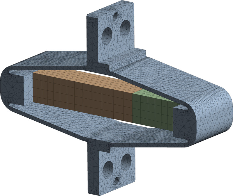
[A] Multi-body simulations with reduced order flexible bodies obtained by FEA
cite:&brumund21_multib_simul_reduc_order_flexib_bodies_fea
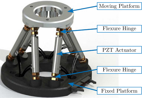
Combined multi-body / FEA techniques and experimental validation on a Stewart platform containing amplified piezoelectric actuators Super-element of amplified piezoelectric actuator / combined multibody-FEA technique, experimental validation on an amplified piezoelectric actuator and further validated on a complete stewart platform
We considered sub-components in the multi-body model as reduced order flexible bodies representing the component’s modal behaviour with reduced mass and stiffness matrices obtained from finite element analysis (FEA) models. These matrices were created from FEA models via modal reduction techniques, more specifically the component mode synthesis (CMS). This makes this design approach a combined multibody-FEA technique. We validated the technique with a test bench that confirmed the good modelling capabilities using reduced order flexible body models obtained from FEA for an amplified piezoelectric actuator (APA).
Robustness by design
- Design of a Stewart platform and associated control architecture that is robust to large plant uncertainties due to large variety of payload and experimental conditions.
- Instead of relying on complex controller synthesis (such as $\mathcal{H}_\infty$ synthesis or $\mu\text{-synthesis}$) to guarantee the robustness and performance.
- The approach here is to choose an adequate architecture (mechanics, sensors, actuators) such that controllers are robust by nature.
- Example: collocated actuator/sensor pair => controller can easily be made robust
- This is done by using models and using HAC-LAC architecture
[A] Mechatronics design
Conduct a rigorous mechatronics design approach for a nano active stabilization system cite:&dehaeze18_sampl_stabil_for_tomog_exper;&dehaeze21_mechat_approac_devel_nano_activ_stabil_system
Approach from start to finish:
- From first concepts using basic models, to concept validation
- Detailed design phase
- Experimental phase
Complete design with clear choices based on models. Such approach, while not new, is here applied This can be used for the design of future end-stations.
% \graphicspath{ {/home/thomas/Cloud/thesis/papers/dehaeze21_mechatronics_approach_nass/tikz/figs-tikz} }

\begin{tikzpicture}
  % Styles
  \tikzset{myblock/.style= {draw, thin, color=white!70!black, fill=white, text width=3cm, align=center, minimum height=1.4cm}};
  \tikzset{mylabel/.style= {anchor=north, below, font=\bfseries\small, color=black, text width=3cm, align=center}};
  \tikzset{mymodel/.style= {anchor=south, above, font=\small, color=black, text width=3cm, align=center}};
  \tikzset{mystep/.style=  {->, ultra thick}};

  % Blocks
  \node[draw, fill=lightblue, align=center, label={[mylabel, text width=8.0cm] Dynamical Models}, minimum height = 4.5cm, text width = 8.0cm] (model) at (0, 0) {};

  \node[myblock, fill=lightgreen, label={[mylabel] Disturbances},  left = 3 of model.west]                          (dist) {};
  \node[myblock, fill=lightgreen, label={[mylabel] Micro Station}, below = 2pt of dist] (mustation) {};
  \node[myblock, fill=lightgreen, label={[mylabel] Nano Hexapod}, above = 2pt of dist] (nanohexapod) {};

  \node[myblock, fill=lightyellow, label={[mylabel] Mech. Design},    above = 1 of model.north] (mechanical) {};
  \node[myblock, fill=lightyellow, label={[mylabel] Instrumentation}, left  = 2pt of mechanical]  (instrumentation) {};
  \node[myblock, fill=lightyellow, label={[mylabel] FEM},             right = 2pt of mechanical]  (fem) {};

  \node[myblock, fill=lightred, label={[mylabel] Test Benches},   right = 3 of model.east]                          (testbenches) {};
  \node[myblock, fill=lightred, label={[mylabel] Assembly},       above = 2pt of testbenches] (mounting) {};
  \node[myblock, fill=lightred, label={[mylabel] Implementation}, below = 2pt of testbenches] (implementation) {};

  % Text
  \node[anchor=south, above, text width=8cm, align=left] at (model.south) {Extensive use of models for:\begin{itemize}[noitemsep,topsep=5pt]\item Extraction of transfer functions \\ \item Choice of appropriate control architecture \\ \item Tuning of control laws \\ \item Closed loop simulations \\ \item Noise budgets / Evaluation of performances \\ \item Sensibility to parameters / disturbances\end{itemize}\centerline{Models are at the core the mecatronic approach!}};

  \node[mymodel] at (mustation.south)       {Multiple stages     \\ Complex dynamics};
  \node[mymodel] at (dist.south)            {Ground motion       \\ Position errors};
  \node[mymodel] at (nanohexapod.south)     {Different concepts  \\ Sensors, Actuators};

  \node[mymodel] at (instrumentation.south) {Sensors, Actuators  \\ Electronics};
  \node[mymodel] at (mechanical.south)      {Proper integration  \\ Ease of assembly};
  \node[mymodel] at (fem.south)             {Optimize key parts: \\ Joints, Plates, APA};

  \node[mymodel] at (mounting.south)        {Struts              \\ Nano-Hexapod};
  \node[mymodel] at (testbenches.south)     {Instrumentation     \\ APA, Struts};
  \node[mymodel] at (implementation.south)  {Control tests       \\ Micro Station};

  % Links
  \draw[->] (dist.east)      -- node[above, midway]{{\small Measurements}} node[below,midway]{{\small Spectral Analysis}} (dist.east-|model.west);
  \draw[->] (mustation.east) -- node[above, midway]{{\small Measurements}} node[below, midway]{{\small CAD Model}} (mustation.east-|model.west);

  \draw[->] ($(nanohexapod.east-|model.west)-(0, 0.15)$) -- node[below, midway]{{\small Optimization}} ($(nanohexapod.east)-(0, 0.15)$);
  \draw[<-] ($(nanohexapod.east-|model.west)+(0, 0.15)$) -- node[above, midway]{{\small Model}} ($(nanohexapod.east)+(0, 0.15)$);

  \draw[->] ($(fem.south|-model.north)+(0.15, 0)$) -- node[right, midway]{{\small Specif.}} ($(fem.south)+(0.15,0)$);
  \draw[<-] ($(fem.south|-model.north)-(0.15, 0)$) -- node[left, midway,align=right]{{\small Super}\\{\small Element}}  ($(fem.south)-(0.15,0)$);

  \draw[->] ($(mechanical.south|-model.north)+(0.15, 0)$) -- node[right, midway]{{\small Specif.}} ($(mechanical.south)+(0.15,0)$);
  \draw[<-] ($(mechanical.south|-model.north)-(0.15, 0)$) -- node[left, midway,align=right]{{\small CAD}\\{\small model}}        ($(mechanical.south)-(0.15,0)$);

  \draw[->] ($(instrumentation.south|-model.north)+(0.15, 0)$) -- node[right, midway]{{\small Specif.}} ($(instrumentation.south)+(0.15,0)$);
  \draw[<-] ($(instrumentation.south|-model.north)-(0.15, 0)$) -- node[left, midway]{{\small Model}}         ($(instrumentation.south)-(0.15,0)$);

  \draw[->] ($(mounting.west-|model.east)+(0, 0.15)$) -- node[above, midway]{{\small Requirements}} ($(mounting.west)+(0, 0.15)$);
  \draw[<-] ($(mounting.west-|model.east)-(0, 0.15)$) -- node[below, midway]{{\small Model refinement}}   ($(mounting.west)-(0, 0.15)$);

  \draw[->] ($(testbenches.west-|model.east)+(0, 0.15)$) -- node[above, midway]{{\small Control Laws}} ($(testbenches.west)+(0, 0.15)$);
  \draw[<-] ($(testbenches.west-|model.east)-(0, 0.15)$) -- node[below, midway]{{\small Model refinement}}   ($(testbenches.west)-(0, 0.15)$);

  \draw[->] ($(implementation.west-|model.east)+(0, 0.15)$) -- node[above, midway]{{\small Control Laws}} ($(implementation.west)+(0, 0.15)$);
  \draw[<-] ($(implementation.west-|model.east)-(0, 0.15)$) -- node[below, midway]{{\small Model refinement}}   ($(implementation.west)-(0, 0.15)$);

  % Main steps
  \node[font=\bfseries, rotate=90, anchor=south, above] (conceptual_phase_node) at (dist.west) {1 - Conceptual Phase};
  \node[font=\bfseries, above] (detailed_phase_node) at (mechanical.north) {2 - Detail Design Phase};
  \node[font=\bfseries, rotate=-90, anchor=south, above] (implementation_phase_node) at (testbenches.east) {3 - Experimental Phase};
    \begin{scope}[on background layer]
      \node[fit={(conceptual_phase_node.north|-nanohexapod.north) (mustation.south east)}, fill=lightgreen!50!white, draw, inner sep=2pt] (conceptual_phase) {};
      \node[fit={(detailed_phase_node.north-|instrumentation.west) (fem.south east)}, fill=lightyellow!50!white, draw, inner sep=2pt] (detailed_phase) {};
      \node[fit={(implementation_phase_node.north|-mounting.north) (implementation.south west)}, fill=lightred!50!white, draw, inner sep=2pt] (implementation_phase) {};
      % \node[above left] at (dob.south east) {DOB};
    \end{scope}

  % Between main steps
  \draw[mystep, postaction={decorate,decoration={raise=1ex,text along path,text align=center,text={Concept Validation}}}] (conceptual_phase.north) to[out=90, in=180] (detailed_phase.west);
  \draw[mystep, postaction={decorate,decoration={raise=1ex,text along path,text align=center,text={Procurement}}}] (detailed_phase.east) to[out=0, in=90] (implementation_phase.north);

  % % Inside Model
  % \node[inner sep=1pt, outer sep=6pt, anchor=north west, draw, fill=white, thin] (multibodymodel) at ($(model.north west) - (0, 0.5)$)
  %   {\includegraphics[width=5.6cm]{simscape_nano_hexapod.png}};

  % \node[inner sep=1pt, outer sep=6pt, anchor=south west, draw, fill=white, thin] (simscape) at (model.south west)
  %   {\includegraphics[width=5.6cm]{simscape_picture.jpg}};

  % % Feedback Model
  % \node[inner sep=3pt, outer sep=6pt, anchor=north east, draw, fill=white, thin] (simscape_sim) at ($(model.north east) - (0, 0.5)$)
  %   {\includegraphics[width=3.6cm]{simscape_simulations.pdf}};

  % % FeedBack
  % \node[inner sep=3pt, outer sep=6pt, anchor=south east, draw, fill=white, thin] (feedback) at (model.south east)
  %   {\includegraphics[width=3.6cm]{classical_feedback_small.pdf}};
\end{tikzpicture}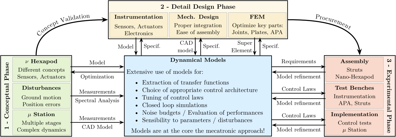
6DoF vibration control of a rotating platform
Vibration control in 5DoF of a rotating stage To the author's knowledge, the use of a continuously rotating stewart platform for vibration control has not been proved in the literature.
Experimental validation of the Nano Active Stabilization System
Demonstration of the improvement of the the positioning accuracy of a complex multi DoF (the micro-station) by several orders of magnitude (Section …) using …
Thesis Outline - Mechatronics Design Approach
Introduction ignore
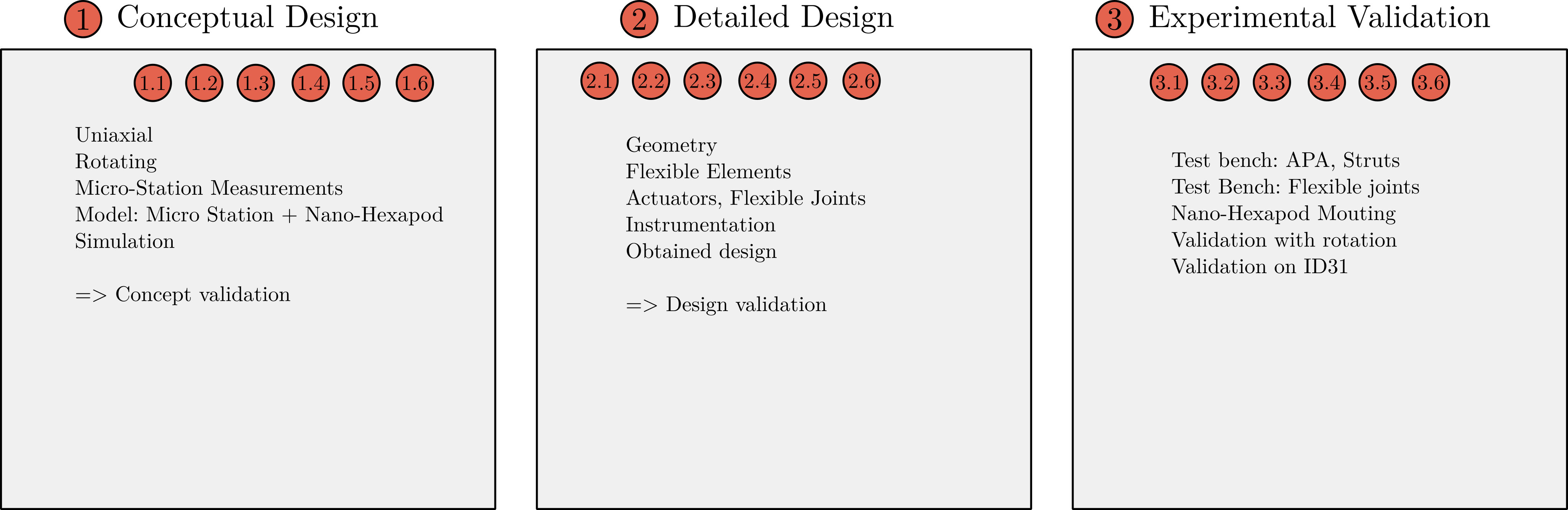
This thesis
- has a structure that follows the mechatronics design approach
Is structured in three chapters that corresponds to the three mains parts of the proposed mechatronics approach.
A brief overview of these three chapters is given bellow.
Conceptual design development
- Start with simple models for witch trade offs can be easily understood (uniaxial)
- Increase the model complexity if important physical phenomenon are to be modelled (cf the rotating model)
- Only when better understanding of the physical effects in play, and only if required, go for higher model complexity (here multi-body model)
- The system concept and main characteristics should be extracted from the different models and validated with closed-loop simulations with the most accurate model
- Once the concept is validated, the chosen concept can be design in mode details
Detailed design
- During this detailed design phase, models are refined from the obtained CAD and using FEM
- The models are used to assists the design and to optimize each element based on dynamical analysis and closed-loop simulations
- The requirements for all the associated instrumentation can be determined from a dynamical noise budgeting
- After converging to a detailed design that give acceptable performance based on the models, the different parts can be ordered and the experimental phase begins
Experimental validation
- It is advised that the important characteristics of the different elements are evaluated individually Systematic validation/refinement of models with experimental measurements
- The obtained characteristics can be used to refine the models
- Then, an accurate model of the system is obtained which can be used during experimental tests (for control synthesis for instance)