Folder name is changed, rework the html templates
Change the organisation.
41 KiB
Measurement Analysis
- Measurement Description
- Importation of the data
- Variables for analysis
- Coherence between the two vertical geophones on the Tilt Stage
- Data Post Processing
- Normalization
- Measurement 1 - Effect of Ty stage
- Measurement 2 - Effect of Ry stage
- Measurement 3 - Effect of the Hexapod
- Measurement 4 - Effect of the Splip-Ring and Spindle
- Measurement 5 - Transmission from ground to marble
Measurement Description
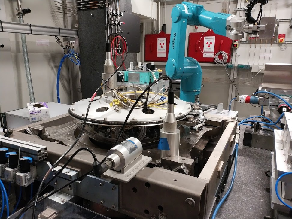
The sensor used are 3 L-4C geophones (Documentation).
Each motor are turn off and then on.
The goal is to see what noise is injected in the system due to the regulation loop of each stage.
Importation of the data
First, load all the measurement files:
  meas = {};
  meas{1} = load('./mat/Measurement1.mat');
  meas{2} = load('./mat/Measurement2.mat');
  meas{3} = load('./mat/Measurement3.mat');
  meas{4} = load('./mat/Measurement4.mat');
  meas{5} = load('./mat/Measurement5.mat');
Change the track name for measurements 3 and 4.
  meas{3}.Track1_Name = 'Input 1: Hexa Z';
  meas{4}.Track1_Name = 'Input 1: Hexa Z';
For the measurements 1 to 4, the measurement channels are shown table tab:meas_14.
| Channel 1 | Channel 2 | Channel 3 | |
|---|---|---|---|
| Meas. 1 | Input 1: tilt1 Z | Input 2: tilt2 Z | Input 3: Ty Y |
| Meas. 2 | Input 1: tilt1 Z | Input 2: tilt2 Z | Input 3: Ty Y |
| Meas. 3 | Input 1: Hexa Z | Input 2: tilt2 Z | Input 3: Ty Y |
| Meas. 4 | Input 1: Hexa Z | Input 2: tilt2 Z | Input 3: Ty Y |
For the measurement 5, the channels are shown table tab:meas_5.
| Channel 1 | Channel 2 | Channel 3 | Channel 4 | |
|---|---|---|---|---|
| Meas. 5 | Input 1: Floor Z | Input 2: Marble Z | Input 3: Floor Y | Input 4: Marble Y |
Variables for analysis
We define the sampling frequency and the time vectors for the plots.
  Fs = 256; % [Hz]
  dt = 1/(Fs);
  t1  = dt*[0:length(meas{1}.Track1)-1];
  t2  = dt*[0:length(meas{2}.Track1)-1];
  t3  = dt*[0:length(meas{3}.Track1)-1];
  t4  = dt*[0:length(meas{4}.Track1)-1];
  t5  = dt*[0:length(meas{5}.Track1)-1];
For the frequency analysis, we define the frequency limits for the plot.
  fmin = 1; % [Hz]
  fmax = 100; % [Hz]
Then we define the windows that will be used to average the results.
psd_window = hanning(2*fmin/dt);Coherence between the two vertical geophones on the Tilt Stage
We first compute the coherence between the two geophones located on the tilt stage. The result is shown on figure fig:coherence_vertical_tilt_sensors.
[coh, f] = mscohere(meas{1}.Track1(:), meas{1}.Track2(:), psd_window, [], [], Fs); <<plt-matlab>>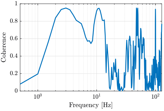
We then compute the transfer function from one sensor to the other (figure fig:tf_vertical_tilt_sensors).
[tf23, f] = tfestimate(meas{1}.Track1(:), meas{1}.Track2(:), psd_window, [], [], Fs); <<plt-matlab>>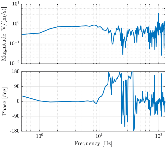
Even though the coherence is not very good, we observe no resonance between the two sensors.
Data Post Processing
When using two geophone sensors on the same tilt stage (measurements 1 and 2), we post-process the data to obtain the z displacement and the rotation of the tilt stage:
  meas1_z    = (meas{1}.Track1+meas{1}.Track2)/2;
  meas1_tilt = (meas{1}.Track1-meas{1}.Track2)/2;

  meas{1}.Track1 = meas1_z;
  meas{1}.Track1_Y_Magnitude = 'Meter / second';
  meas{1}.Track1_Name = 'Ry Z';
  meas{1}.Track2 = meas1_tilt;
  meas{1}.Track2_Y_Magnitude = 'Rad / second';
  meas{1}.Track2_Name = 'Ry Tilt';

  meas2_z    = (meas{2}.Track1+meas{2}.Track2)/2;
  meas2_tilt = (meas{2}.Track1-meas{2}.Track2)/2;
  meas{2}.Track1 = meas2_z;
  meas{2}.Track1_Y_Magnitude = 'Meter / second';
  meas{2}.Track1_Name = 'Ry Z';
  meas{2}.Track2 = meas2_tilt;
  meas{2}.Track2_Y_Magnitude = 'Rad / second';
  meas{2}.Track2_Name = 'Ry Tilt';
Normalization
Parameters of the geophone are defined below. The transfer function from geophone velocity to measured voltage is shown on figure fig:L4C_bode_plot.
Measurements will be normalized by the inverse of this transfer function in order to go from voltage measurement to velocity measurement.
  L4C_w0 = 2*pi; % [rad/s]
  L4C_ksi = 0.28;
  L4C_G0 = 276.8; % [V/(m/s)]
L4C_G = L4C_G0*(s/L4C_w0)^2/((s/L4C_w0)^2 + 2*L4C_ksi*(s/L4C_w0) + 1); <<plt-matlab>>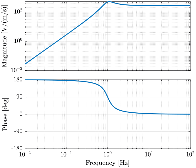
  meas{1}.Track1 = (meas{1}.Track1)./276.8;
  meas{1}.Track2 = (meas{1}.Track2)./276.8;
  meas{1}.Track3 = (meas{1}.Track3)./276.8;

  meas{2}.Track1 = (meas{2}.Track1)./276.8;
  meas{2}.Track2 = (meas{2}.Track2)./276.8;
  meas{2}.Track3 = (meas{2}.Track3)./276.8;

  meas{3}.Track1 = (meas{3}.Track1)./276.8;
  meas{3}.Track2 = (meas{3}.Track2)./276.8;
  meas{3}.Track3 = (meas{3}.Track3)./276.8;

  meas{4}.Track1 = (meas{4}.Track1)./276.8;
  meas{4}.Track2 = (meas{4}.Track2)./276.8;
  meas{4}.Track3 = (meas{4}.Track3)./276.8;

  meas{5}.Track1 = (meas{5}.Track1)./276.8;
  meas{5}.Track2 = (meas{5}.Track2)./276.8;
  meas{5}.Track3 = (meas{5}.Track3)./276.8;
meas{5}.Track4 = (meas{5}.Track4)./276.8; meas{1}.Track1_norm = lsim(inv(L4C_G), meas{1}.Track1, t1);
meas{1}.Track2_norm = lsim(inv(L4C_G), meas{1}.Track2, t1);
meas{1}.Track3_norm = lsim(inv(L4C_G), meas{1}.Track3, t1);
meas{2}.Track1_norm = lsim(inv(L4C_G), meas{2}.Track1, t2);
meas{2}.Track2_norm = lsim(inv(L4C_G), meas{2}.Track2, t2);
meas{2}.Track3_norm = lsim(inv(L4C_G), meas{2}.Track3, t2);
meas{3}.Track1_norm = lsim(inv(L4C_G), meas{3}.Track1, t3);
meas{3}.Track2_norm = lsim(inv(L4C_G), meas{3}.Track2, t3);
meas{3}.Track3_norm = lsim(inv(L4C_G), meas{3}.Track3, t3);
meas{4}.Track1_norm = lsim(inv(L4C_G), meas{4}.Track1, t4);
meas{4}.Track2_norm = lsim(inv(L4C_G), meas{4}.Track2, t4);
meas{4}.Track3_norm = lsim(inv(L4C_G), meas{4}.Track3, t4);
meas{5}.Track1_norm = lsim(inv(L4C_G), meas{5}.Track1, t5);
meas{5}.Track2_norm = lsim(inv(L4C_G), meas{5}.Track2, t5);
meas{5}.Track3_norm = lsim(inv(L4C_G), meas{5}.Track3, t5);
meas{5}.Track4_norm = lsim(inv(L4C_G), meas{5}.Track4, t5);Measurement 1 - Effect of Ty stage
The configuration for this measurement is shown table tab:conf_meas1.
| Time | 0-309 | 309-end |
|---|---|---|
| Ty | OFF | ON |
| Ry | OFF | OFF |
| SlipRing | OFF | OFF |
| Spindle | OFF | OFF |
| Hexa | OFF | OFF |
We then plot the measurements in time domain (figure fig:meas1).
We observe strange behavior when the Ty stage is turned on. How can we explain that?
<<plt-matlab>>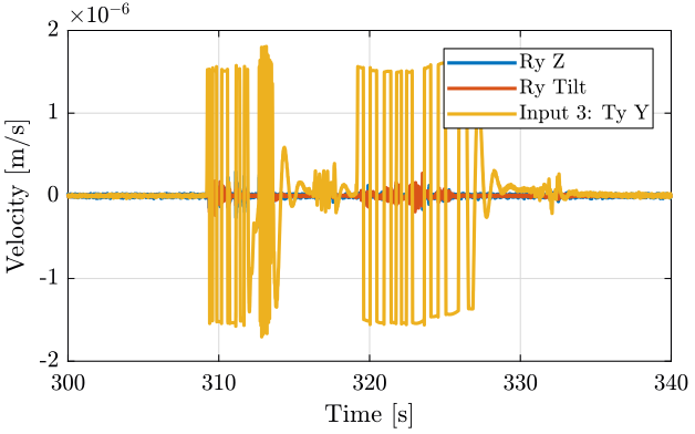
To understand what is going on, instead of looking at the velocity, we can look at the displacement by integrating the data. The displacement is computed by integrating the velocity using cumtrapz function.
Then we plot the position with respect to time (figure fig:meas1_disp).
<<plt-matlab>>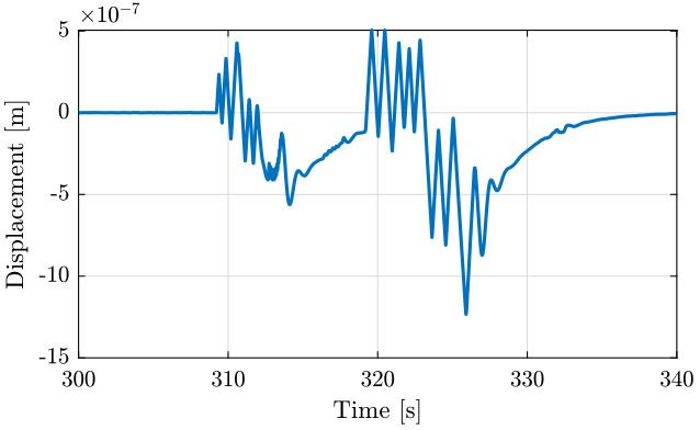
We when compute the power spectral density of each measurement before and after turning on the stage.
  [pxx111, f11] = pwelch(meas{1}.Track1(1:ceil(300/dt)),   psd_window, [], [], Fs);
  [pxx112, f12] = pwelch(meas{1}.Track1(ceil(350/dt):end), psd_window, [], [], Fs);

  [pxx121, ~] = pwelch(meas{1}.Track2(1:ceil(300/dt)),   psd_window, [], [], Fs);
  [pxx122, ~] = pwelch(meas{1}.Track2(ceil(350/dt):end), psd_window, [], [], Fs);

  [pxx131, ~] = pwelch(meas{1}.Track3(1:ceil(300/dt)),   psd_window, [], [], Fs);
  [pxx132, ~] = pwelch(meas{1}.Track3(ceil(350/dt):end), psd_window, [], [], Fs);
We finally plot the power spectral density of each track (figures fig:meas1_ry_z_psd, fig:meas1_ry_tilt_psd, fig:meas1_ty_y_psd).
<<plt-matlab>>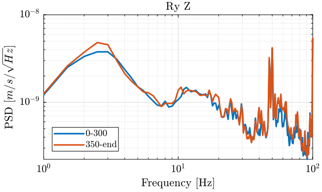
<<plt-matlab>>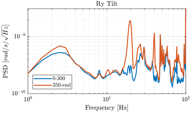
<<plt-matlab>>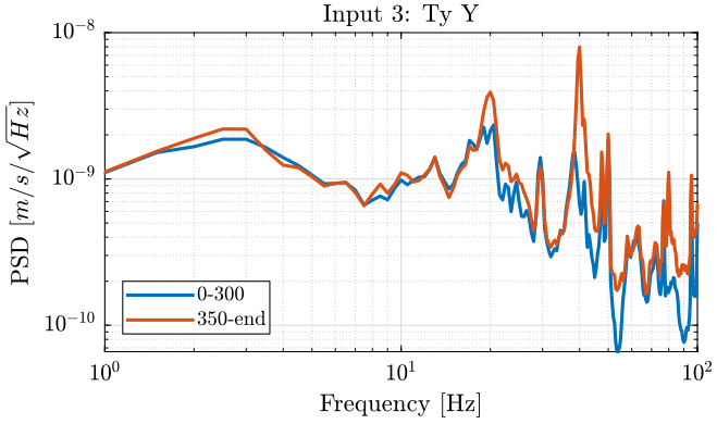
Turning on the Y-translation stage increases the velocity of the Ty stage in the Y direction and the rotation motion of the tilt stage:
- at 20Hz
- at 40Hz
- between 80Hz and 90Hz
It does not seems to have any effect on the Z motion of the tilt stage.
Measurement 2 - Effect of Ry stage
The tilt stage is turned ON at around 326 seconds (table tab:conf_meas2).
| Time | 0-326 | 326-end |
|---|---|---|
| Ty | OFF | OFF |
| Ry | OFF | ON |
| SlipRing | OFF | OFF |
| Spindle | OFF | OFF |
| Hexa | OFF | OFF |
We plot the time domain (figure fig:meas2) and we don't observe anything special in the time domain.
<<plt-matlab>>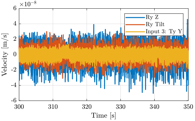
<<plt-matlab>>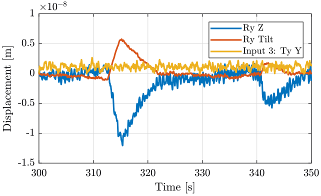
We compute the PSD of each track and we plot them (figures fig:meas2_ry_z_psd, fig:meas2_ry_tilt_psd and fig:meas2_ty_y_psd ).
  [pxx211, f21] = pwelch(meas{2}.Track1(1:ceil(326/dt)),   psd_window, [], [], Fs);
  [pxx212, f22] = pwelch(meas{2}.Track1(ceil(326/dt):end), psd_window, [], [], Fs);

  [pxx221, ~] = pwelch(meas{2}.Track2(1:ceil(326/dt)),   psd_window, [], [], Fs);
  [pxx222, ~] = pwelch(meas{2}.Track2(ceil(326/dt):end), psd_window, [], [], Fs);

  [pxx231, ~] = pwelch(meas{2}.Track3(1:ceil(326/dt)),   psd_window, [], [], Fs);
[pxx232, ~] = pwelch(meas{2}.Track3(ceil(326/dt):end), psd_window, [], [], Fs); <<plt-matlab>>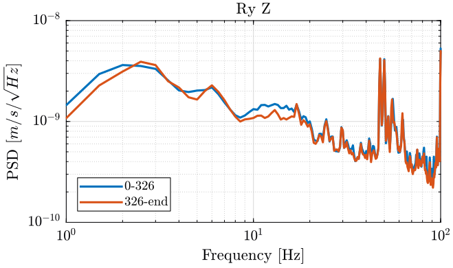
<<plt-matlab>>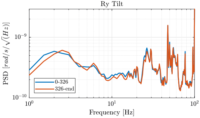
<<plt-matlab>>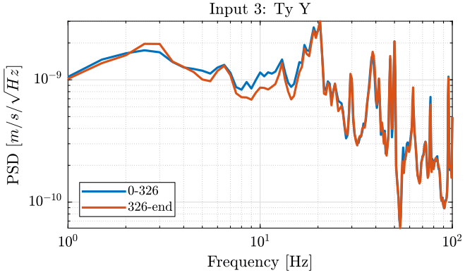
We observe no noticeable difference when the Tilt-stage is turned ON expect a small decrease of the Z motion of the tilt stage around 10Hz.
Measurement 3 - Effect of the Hexapod
The hexapod is turned off after 406 seconds (table tab:conf_meas3).
| Time | 0-406 | 406-end |
|---|---|---|
| Ty | OFF | OFF |
| Ry | ON | ON |
| SlipRing | OFF | OFF |
| Spindle | OFF | OFF |
| Hexa | ON | OFF |
The time domain result is shown figure fig:meas3.
<<plt-matlab>>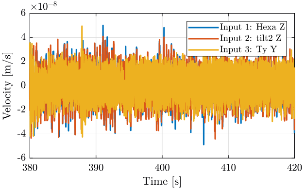
<<plt-matlab>>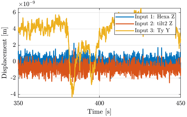
We then compute the PSD of each track before and after turning off the hexapod and plot the results in the figures fig:meas3_hexa_z_psd, fig:meas3_ry_z_psd and fig:meas3_ty_y_psd.
  [pxx311, f31] = pwelch(meas{3}.Track1(1:ceil(400/dt)),   psd_window, [], [], Fs);
  [pxx312, f32] = pwelch(meas{3}.Track1(ceil(420/dt):end), psd_window, [], [], Fs);

  [pxx321, ~] = pwelch(meas{3}.Track2(1:ceil(400/dt)),   psd_window, [], [], Fs);
  [pxx322, ~] = pwelch(meas{3}.Track2(ceil(420/dt):end), psd_window, [], [], Fs);

  [pxx331, ~] = pwelch(meas{3}.Track3(1:ceil(400/dt)),   psd_window, [], [], Fs);
[pxx332, ~] = pwelch(meas{3}.Track3(ceil(420/dt):end), psd_window, [], [], Fs); <<plt-matlab>>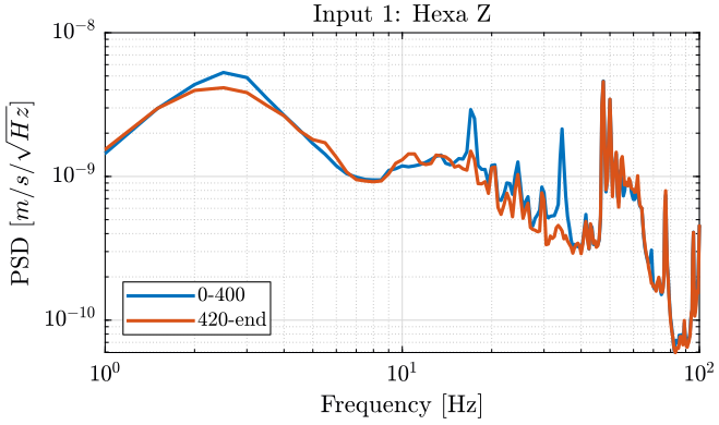
<<plt-matlab>>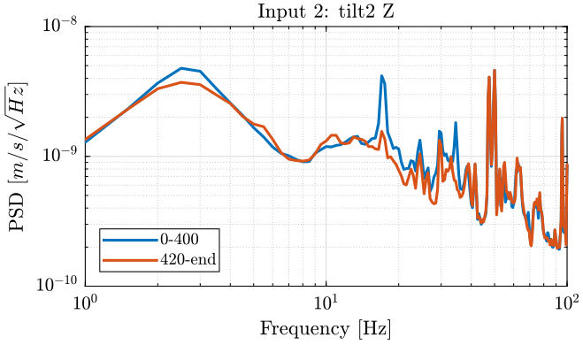
<<plt-matlab>>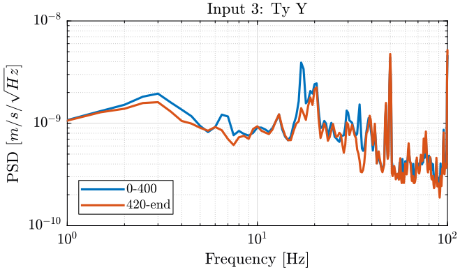
Turning ON induces some motion on the hexapod in the z direction (figure fig:meas3_hexa_z_psd), on the tilt stage in the z direction (figure fig:meas3_ry_z_psd) and on the y motion of the Ty stage (figure fig:meas3_ty_y_psd):
- at 17Hz
- at 34Hz
Measurement 4 - Effect of the Splip-Ring and Spindle
The slip ring is turned on at 300s, then the spindle is turned on at 620s (table tab:conf_meas4). The time domain signals are shown figure fig:meas4.
| Time | 0-300 | 300-620 | 620-end |
|---|---|---|---|
| Ty | OFF | OFF | OFF |
| Ry | OFF | OFF | OFF |
| SlipRing | OFF | ON | ON |
| Spindle | OFF | OFF | ON |
| Hexa | OFF | OFF | OFF |
<<plt-matlab>>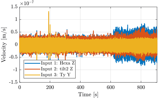
If we integrate this signal, we obtain Figure fig:meas4_int.
<<plt-matlab>>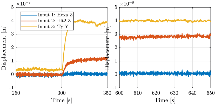
The PSD of each track are computed using the code below.
<<plt-matlab>>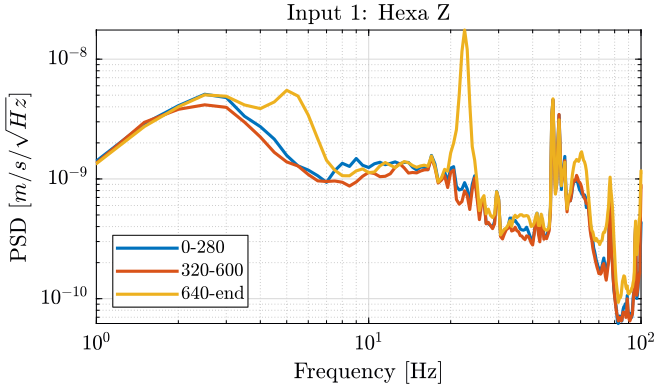
We plot the PSD of the displacement.
<<plt-matlab>>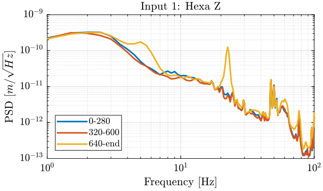
And we compute the Cumulative amplitude spectrum.
<<plt-matlab>>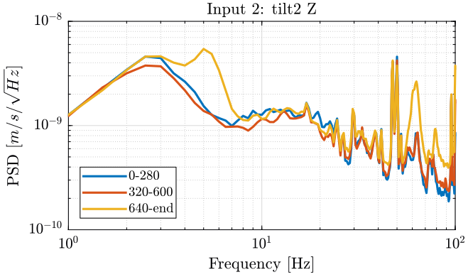
<<plt-matlab>>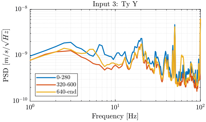
Turning ON the splipring seems to not add motions on the stages measured. It even seems to lower the motion of the Ty stage (figure fig:meas4_ty_y_psd): does that make any sense?
Turning ON the spindle induces motions:
- at 5Hz on each motion measured
- at 22.5Hz on the Z motion of the Hexapod. Can this is due to some 50Hz?
- at 62Hz on each motion measured
Measurement 5 - Transmission from ground to marble
This measurement just consists of measurement of Y-Z motion of the ground and the marble.
The time domain signals are shown on figure fig:meas5.
<<plt-matlab>>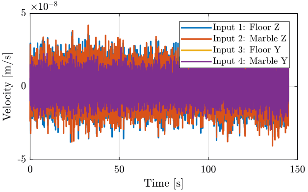
We compute the PSD of each track and we plot the PSD of the Z motion for the ground and marble on figure fig:meas5_z_psd and for the Y motion on figure fig:meas5_y_psd.
  [pxx51, f51] = pwelch(meas{5}.Track1(:), psd_window, [], [], Fs);
  [pxx52, f52] = pwelch(meas{5}.Track2(:), psd_window, [], [], Fs);
  [pxx53, f53] = pwelch(meas{5}.Track3(:), psd_window, [], [], Fs);
[pxx54, f54] = pwelch(meas{5}.Track4(:), psd_window, [], [], Fs); <<plt-matlab>>
<<plt-matlab>>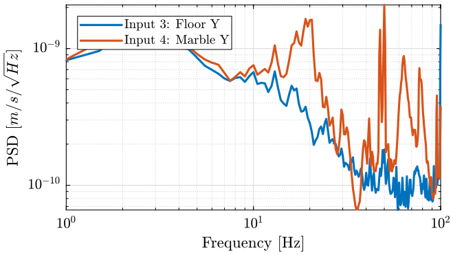
Then, instead of looking at the Power Spectral Density, we can try to estimate the transfer function from a ground motion to the motion of the marble. The transfer functions are shown on figure fig:meas5_tf and the coherence on figure fig:meas5_coh.
  [tfz, fz] = tfestimate(meas{5}.Track1(:), meas{5}.Track2(:), psd_window, [], [], Fs);
[tfy, fy] = tfestimate(meas{5}.Track3(:), meas{5}.Track4(:), psd_window, [], [], Fs); <<plt-matlab>>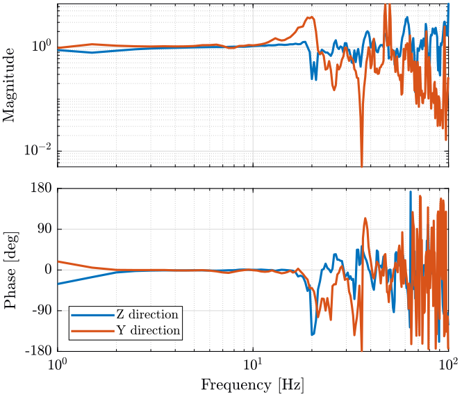
  [cohz, fz] = mscohere(meas{5}.Track1(:), meas{5}.Track2(:), psd_window, [], [], Fs);
[cohy, fy] = mscohere(meas{5}.Track3(:), meas{5}.Track4(:), psd_window, [], [], Fs); <<plt-matlab>>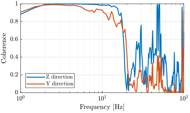
The marble seems to have a resonance at around 20Hz on the Y direction. But the coherence is not good above 20Hz, so it is difficult to estimate resonances.