17 KiB
Measurements on the instrumentation
- Measure of the noise of the Voltage Amplifier
- Measure of the influence of the AC/DC option on the voltage amplifiers
- Transfer function of the Low Pass Filter
Measure of the noise of the Voltage Amplifier
<<sec:meas_volt_amp>>
ZIP file containing the data and matlab files ignore
All the files (data and Matlab scripts) are accessible here.
Measurement Description
Goal:
- Determine the Voltage Amplifier noise
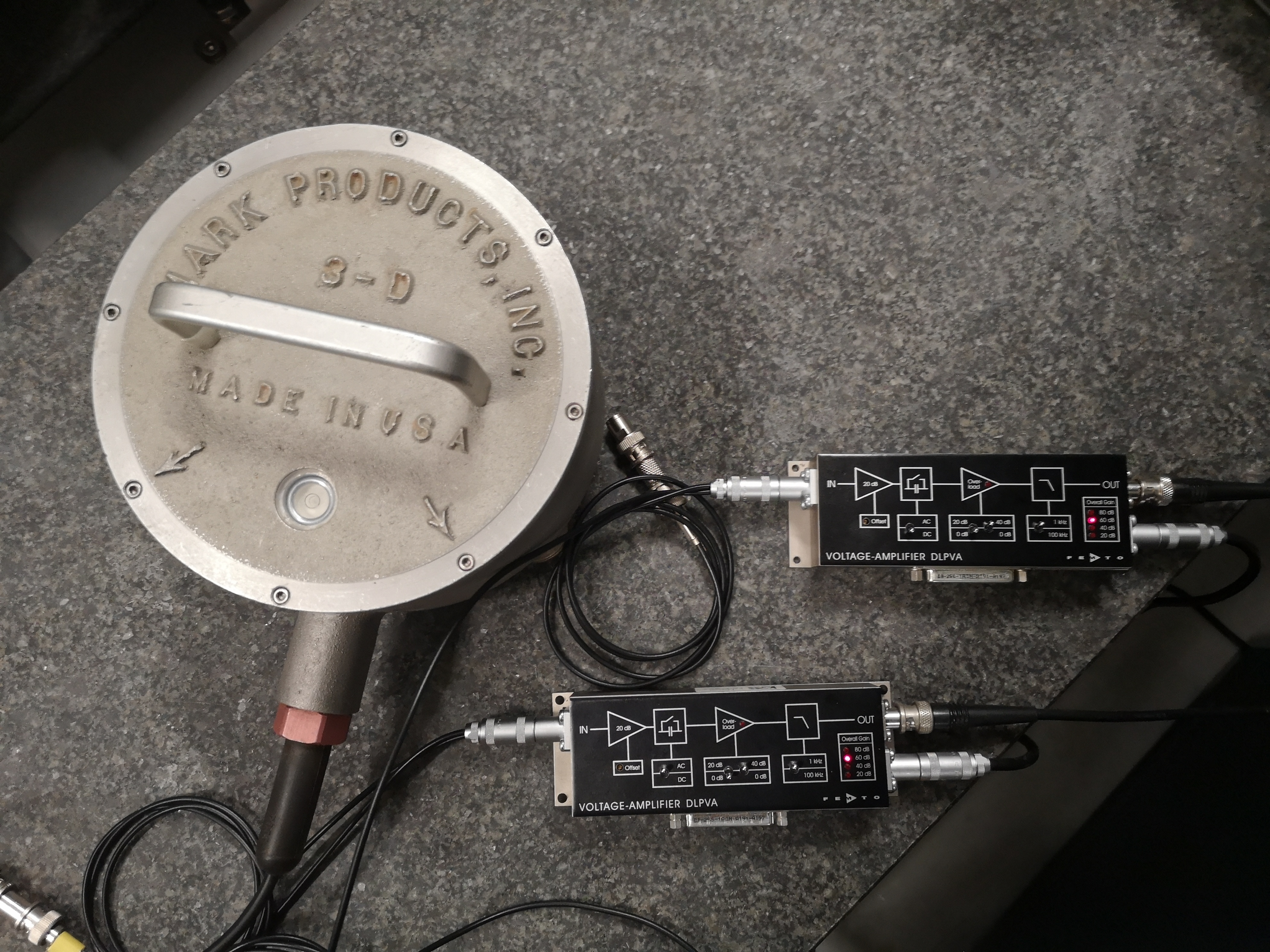
Setup:
- The two inputs (differential) of the voltage amplifier are shunted with 50Ohms
- The AC/DC option of the Voltage amplifier is on AC
- The low pass filter is set to 1hHz
- We measure the output of the voltage amplifier with a 16bits ADC of the Speedgoat
Measurements:
data_003: Ampli OFFdata_004: Ampli ON set to 20dBdata_005: Ampli ON set to 40dBdata_006: Ampli ON set to 60dB
Load data
  amp_off = load('mat/data_003.mat', 'data'); amp_off = amp_off.data(:, [1,3]);
  amp_20d = load('mat/data_004.mat', 'data'); amp_20d = amp_20d.data(:, [1,3]);
  amp_40d = load('mat/data_005.mat', 'data'); amp_40d = amp_40d.data(:, [1,3]);
  amp_60d = load('mat/data_006.mat', 'data'); amp_60d = amp_60d.data(:, [1,3]);
Time Domain
The time domain signals are shown on figure fig:ampli_noise_time.
<<plt-matlab>>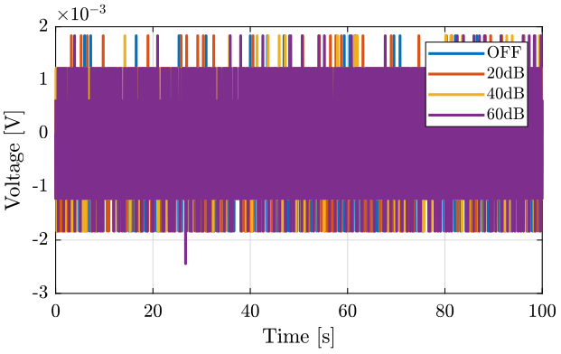
Frequency Domain
We first compute some parameters that will be used for the PSD computation.
  dt = amp_off(2, 2)-amp_off(1, 2);

  Fs = 1/dt; % [Hz]

  win = hanning(ceil(10*Fs));
Then we compute the Power Spectral Density using pwelch function.
  [pxoff, f] = pwelch(amp_off(:,1), win, [], [], Fs);
  [px20d, ~] = pwelch(amp_20d(:,1), win, [], [], Fs);
  [px40d, ~] = pwelch(amp_40d(:,1), win, [], [], Fs);
  [px60d, ~] = pwelch(amp_60d(:,1), win, [], [], Fs);
We compute the theoretical ADC noise.
  q = 20/2^16; % quantization
  Sq = q^2/12/1000; % PSD of the ADC noise
Finally, the ASD is shown on figure fig:ampli_noise_psd.
<<plt-matlab>>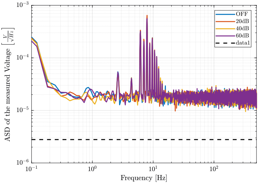
Conclusion
Questions:
- Where does those sharp peaks comes from? Can this be due to aliasing?
Noise induced by the voltage amplifiers seems not to be a limiting factor as we have the same noise when they are OFF and ON.
Measure of the influence of the AC/DC option on the voltage amplifiers
<<sec:meas_noise_ac_dc>>
ZIP file containing the data and matlab files ignore
All the files (data and Matlab scripts) are accessible here.
Measurement Description
Goal:
- Measure the influence of the high-pass filter option of the voltage amplifiers
Setup:
- One geophone is located on the marble.
- It's signal goes to two voltage amplifiers with a gain of 60dB.
- One voltage amplifier is on the AC option, the other is on the DC option.
Measurements:
First measurement (mat/data_014.mat file):
| Column | Signal |
|---|---|
| 1 | Amplifier 1 with AC option |
| 2 | Amplifier 2 with DC option |
| 3 | Time |
Second measurement (mat/data_015.mat file):
| Column | Signal |
|---|---|
| 1 | Amplifier 1 with DC option |
| 2 | Amplifier 2 with AC option |
| 3 | Time |
Load data
We load the data of the z axis of two geophones.
  meas14 = load('mat/data_014.mat', 'data'); meas14 = meas14.data;
  meas15 = load('mat/data_015.mat', 'data'); meas15 = meas15.data;
Time Domain
The signals are shown on figure fig:ac_dc_option_time.
<<plt-matlab>>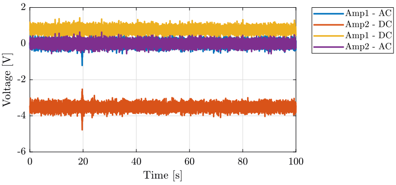
Frequency Domain
We first compute some parameters that will be used for the PSD computation.
  dt = meas14(2, 3)-meas14(1, 3);

  Fs = 1/dt; % [Hz]

  win = hanning(ceil(10*Fs));
Then we compute the Power Spectral Density using pwelch function.
  [pxamp1ac, f] = pwelch(meas14(:, 1), win, [], [], Fs);
  [pxamp2dc, ~] = pwelch(meas14(:, 2), win, [], [], Fs);

  [pxamp1dc, ~] = pwelch(meas15(:, 1), win, [], [], Fs);
  [pxamp2ac, ~] = pwelch(meas15(:, 2), win, [], [], Fs);
The ASD of the signals are compare on figure fig:ac_dc_option_asd.
<<plt-matlab>>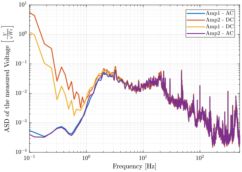
Conclusion
- The voltage amplifiers include some very sharp high pass filters at 1.5Hz (maybe 4th order)
- There is a DC offset on the time domain signal because the DC-offset knob was not set to zero
Transfer function of the Low Pass Filter
<<sec:low_pass_filter_measurements>>
ZIP file containing the data and matlab files ignore
The computation files for this section are accessible here.
First LPF with a Cut-off frequency of 160Hz
Measurement Description
Goal:
- Measure the Low Pass Filter Transfer Function
The values of the components are:
\begin{aligned} R &= 1k\Omega \\ C &= 1\mu F \end{aligned}Which makes a cut-off frequency of $f_c = \frac{1}{RC} = 1000 rad/s = 160Hz$.
  \begin{tikzpicture}
    \draw (0,2)
          to [R=\(R\)] ++(2,0) node[circ]
          to ++(2,0)
          ++(-2,0)
          to [C=\(C\)] ++(0,-2) node[circ]
          ++(-2,0)
          to ++(2,0)
          to ++(2,0)
  \end{tikzpicture}
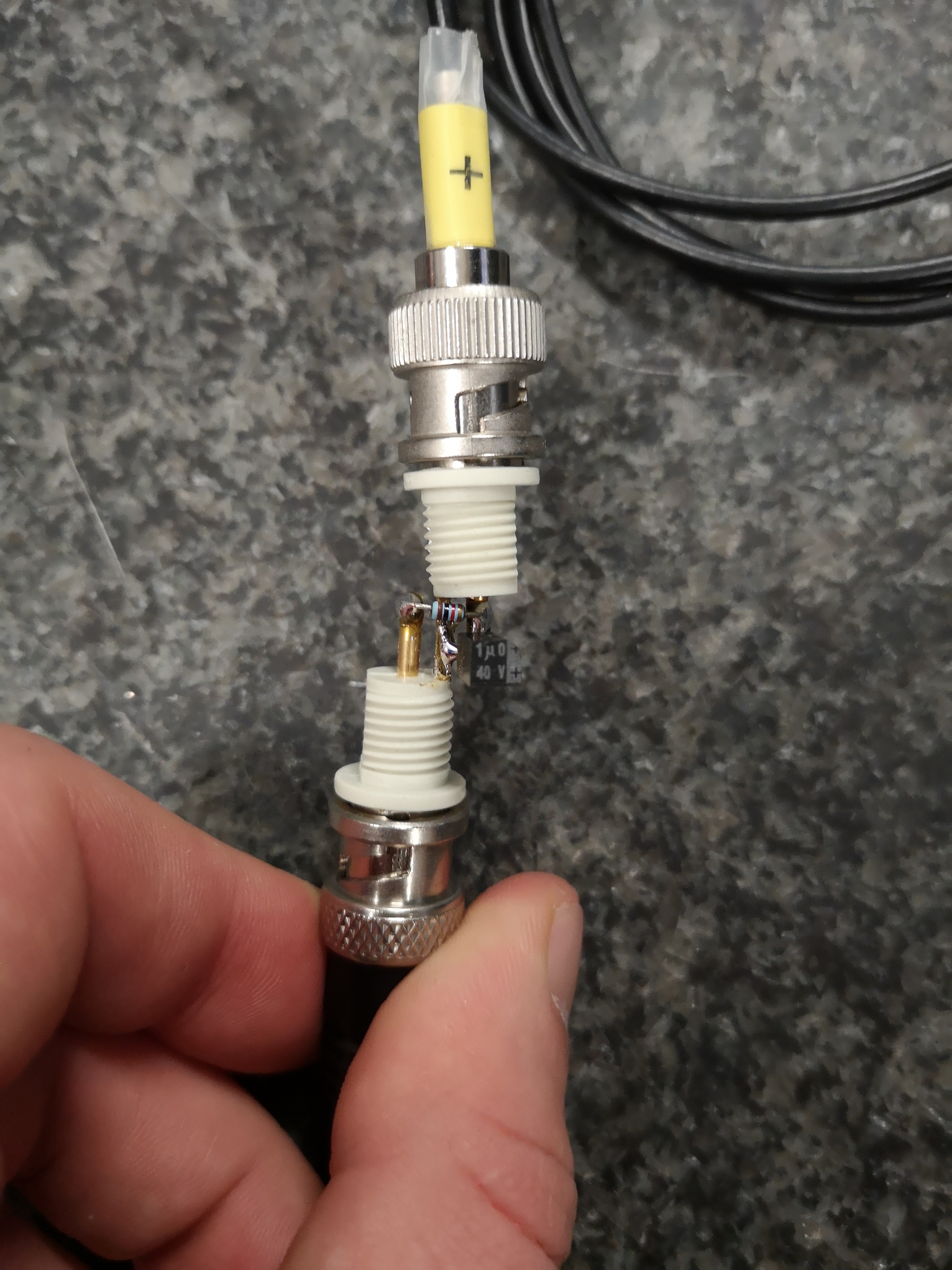
Setup:
- We are measuring the signal from from Geophone with a BNC T
- On part goes to column 1 through the LPF
- The other part goes to column 2 without the LPF
Measurements:
mat/data_018.mat:
| Column | Signal |
|---|---|
| 1 | Amplifier 1 with LPF |
| 2 | Amplifier 2 |
| 3 | Time |
Load data
We load the data of the z axis of two geophones.
data = load('mat/data_018.mat', 'data'); data = data.data;Transfer function of the LPF
We compute the transfer function from the signal without the LPF to the signal measured with the LPF.
  dt = data(2, 3)-data(1, 3);

  Fs = 1/dt; % [Hz]

win = hanning(ceil(10*Fs)); [Glpf, f] = tfestimate(data(:, 2), data(:, 1), win, [], [], Fs);We compare this transfer function with a transfer function corresponding to an ideal first order LPF with a cut-off frequency of $1000rad/s$. We obtain the result on figure fig:Glpf_bode.
Gth = 1/(1+s/1000) figure;
ax1 = subplot(2, 1, 1);
hold on;
plot(f, abs(Glpf));
plot(f, abs(squeeze(freqresp(Gth, f, 'Hz'))));
hold off;
set(gca, 'xscale', 'log'); set(gca, 'yscale', 'log');
set(gca, 'XTickLabel',[]);
ylabel('Magnitude');
ax2 = subplot(2, 1, 2);
hold on;
plot(f, mod(180+180/pi*phase(Glpf), 360)-180);
plot(f, 180/pi*unwrap(angle(squeeze(freqresp(Gth, f, 'Hz')))));
hold off;
set(gca, 'xscale', 'log');
ylim([-180, 180]);
yticks([-180, -90, 0, 90, 180]);
xlabel('Frequency [Hz]'); ylabel('Phase');
linkaxes([ax1,ax2],'x');
xlim([1, 500]); <<plt-matlab>>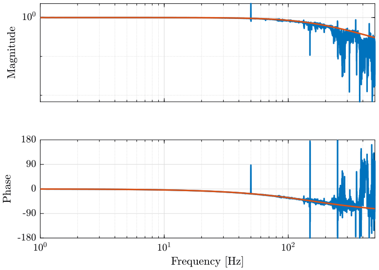
Conclusion
As we want to measure things up to $500Hz$, we chose to change the value of the capacitor to obtain a cut-off frequency of $1kHz$.
Second LPF with a Cut-off frequency of 1000Hz
Measurement description
This time, the value are
\begin{aligned} R &= 1k\Omega \\ C &= 150nF \end{aligned}Which makes a low pass filter with a cut-off frequency of $f_c = 1060Hz$.
Load data
We load the data of the z axis of two geophones.
data = load('mat/data_019.mat', 'data'); data = data.data;Transfer function of the LPF
We compute the transfer function from the signal without the LPF to the signal measured with the LPF.
  dt = data(2, 3)-data(1, 3);

  Fs = 1/dt; % [Hz]

win = hanning(ceil(10*Fs)); [Glpf, f] = tfestimate(data(:, 2), data(:, 1), win, [], [], Fs);We compare this transfer function with a transfer function corresponding to an ideal first order LPF with a cut-off frequency of $1060Hz$. We obtain the result on figure fig:Glpf_bode_bis.
Gth = 1/(1+s/1060/2/pi); figure;
ax1 = subplot(2, 1, 1);
hold on;
plot(f, abs(Glpf));
plot(f, abs(squeeze(freqresp(Gth, f, 'Hz'))));
hold off;
set(gca, 'xscale', 'log'); set(gca, 'yscale', 'log');
set(gca, 'XTickLabel',[]);
ylabel('Magnitude');
ax2 = subplot(2, 1, 2);
hold on;
plot(f, mod(180+180/pi*phase(Glpf), 360)-180);
plot(f, 180/pi*unwrap(angle(squeeze(freqresp(Gth, f, 'Hz')))));
hold off;
set(gca, 'xscale', 'log');
ylim([-180, 180]);
yticks([-180, -90, 0, 90, 180]);
xlabel('Frequency [Hz]'); ylabel('Phase');
linkaxes([ax1,ax2],'x');
xlim([1, 500]); <<plt-matlab>>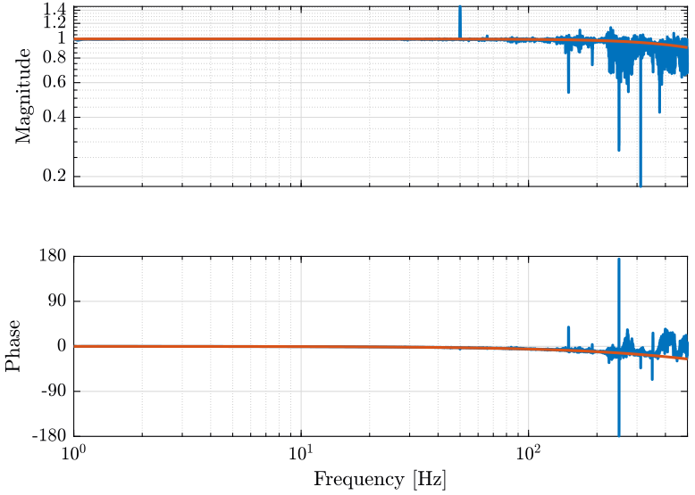
Conclusion
The added LPF has the expected behavior.