26 KiB
26 KiB
Complementary Filters Shaping Using $\mathcal{H}_\infty$ Synthesis - Tikz Figures
- Fig 1: Sensor Fusion Architecture
- Fig 2: Sensor fusion architecture with sensor dynamics uncertainty
- Fig 3: Uncertainty set of the super sensor dynamics
- Fig 4: Architecture used for $\mathcal{H}_\infty$ synthesis of complementary filters
- Fig 5: Magnitude of a weighting function generated using the proposed formula
- Fig 6: Frequency response of the weighting functions and complementary filters obtained using $\mathcal{H}_\infty$ synthesis
- Fig 7: Architecture for $\mathcal{H}_\infty$ synthesis of three complementary filters
- Fig 8: Frequency response of the weighting functions and three complementary filters obtained using $\mathcal{H}_\infty$ synthesis
- Fig 9: Specifications and weighting functions magnitude used for $\mathcal{H}_\infty$ synthesis
- Fig 10: Comparison of the FIR filters (solid) with the filters obtained with $\mathcal{H}_\infty$ synthesis (dashed)
Configuration file is accessible here.
Fig 1: Sensor Fusion Architecture
  \begin{tikzpicture}
    \node[branch] (x) at (0, 0);
    \node[block, above right=0.5 and 0.5 of x](G1){$G_1(s)$};
    \node[block, below right=0.5 and 0.5 of x](G2){$G_2(s)$};
    \node[addb, right=0.8 of G1](add1){};
    \node[addb, right=0.8 of G2](add2){};
    \node[block, right=0.8 of add1](H1){$H_1(s)$};
    \node[block, right=0.8 of add2](H2){$H_2(s)$};
    \node[addb, right=5 of x](add){};

    \draw[] ($(x)+(-0.7, 0)$) node[above right]{$x$} -- (x.center);
    \draw[->] (x.center) |- (G1.west);
    \draw[->] (x.center) |- (G2.west);
    \draw[->] (G1.east) -- (add1.west);
    \draw[->] (G2.east) -- (add2.west);
    \draw[<-] (add1.north) -- ++(0, 0.8)node[below right](n1){$n_1$};
    \draw[<-] (add2.north) -- ++(0, 0.8)node[below right](n2){$n_2$};
    \draw[->] (add1.east) -- (H1.west);
    \draw[->] (add2.east) -- (H2.west);
    \draw[->] (H1) -| (add.north);
    \draw[->] (H2) -| (add.south);
    \draw[->] (add.east) -- ++(0.7, 0) node[above left]{$\hat{x}$};

    \begin{scope}[on background layer]
      \node[fit={($(G2.south-|x)+(-0.2, -0.3)$) ($(n1.north east-|add.east)+(0.2, 0.3)$)}, fill=black!10!white, draw, dashed, inner sep=0pt] (supersensor) {};
      \node[below left] at (supersensor.north east) {Super Sensor};

      \node[fit={($(G1.south west)+(-0.3, -0.1)$) ($(n1.north east)+(0.0, 0.1)$)}, fill=black!20!white, draw, dashed, inner sep=0pt] (sensor1) {};
      \node[below right] at (sensor1.north west) {Sensor 1};
      \node[fit={($(G2.south west)+(-0.3, -0.1)$) ($(n2.north east)+(0.0, 0.1)$)}, fill=black!20!white, draw, dashed, inner sep=0pt] (sensor2) {};
      \node[below right] at (sensor2.north west) {Sensor 2};
    \end{scope}
  \end{tikzpicture}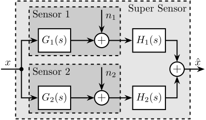
Fig 2: Sensor fusion architecture with sensor dynamics uncertainty
  \begin{tikzpicture}
    \node[branch] (x) at (0, 0);
    \node[addb, above right=0.8 and 4 of x](add1){};
    \node[addb, below right=0.8 and 4 of x](add2){};
    \node[block, above left=0.2 and 0.1 of add1](delta1){$\Delta_1(s)$};
    \node[block, above left=0.2 and 0.1 of add2](delta2){$\Delta_2(s)$};
    \node[block, left=0.5 of delta1](W1){$w_1(s)$};
    \node[block, left=0.5 of delta2](W2){$w_2(s)$};
    \node[block, right=0.5 of add1](H1){$H_1(s)$};
    \node[block, right=0.5 of add2](H2){$H_2(s)$};
    \node[addb, right=6 of x](add){};

    \draw[] ($(x)+(-0.7, 0)$) node[above right]{$x$} -- (x.center);
    \draw[->] (x.center) |- (add1.west);
    \draw[->] (x.center) |- (add2.west);
    \draw[->] ($(add1-|W1.west)+(-0.5, 0)$)node[branch](S1){} |- (W1.west);
    \draw[->] ($(add2-|W2.west)+(-0.5, 0)$)node[branch](S1){} |- (W2.west);
    \draw[->] (W1.east) -- (delta1.west);
    \draw[->] (W2.east) -- (delta2.west);
    \draw[->] (delta1.east) -| (add1.north);
    \draw[->] (delta2.east) -| (add2.north);
    \draw[->] (add1.east) -- (H1.west);
    \draw[->] (add2.east) -- (H2.west);
    \draw[->] (H1.east) -| (add.north);
    \draw[->] (H2.east) -| (add.south);
    \draw[->] (add.east) -- ++(0.7, 0) node[above left]{$\hat{x}$};

    \begin{scope}[on background layer]
      \node[block, fit={($(W1.north-|S1)+(-0.2, 0.2)$) ($(add1.south east)+(0.2, -0.3)$)}, fill=black!20!white, dashed, inner sep=0pt] (sensor1) {};
      \node[above right] at (sensor1.south west) {Sensor 1};
      \node[block, fit={($(W2.north-|S1)+(-0.2, 0.2)$) ($(add2.south east)+(0.2, -0.3)$)}, fill=black!20!white, dashed, inner sep=0pt] (sensor2) {};
      \node[above right] at (sensor2.south west) {Sensor 2};
    \end{scope}
  \end{tikzpicture}
Fig 3: Uncertainty set of the super sensor dynamics
  \begin{tikzpicture}
    \begin{scope}[shift={(4, 0)}]

      % Uncertainty Circle
      \node[draw, circle, fill=black!20!white, minimum size=3.6cm] (c) at (0, 0) {};
      \path[draw, dotted] (0, 0) circle [radius=1.0];
      \path[draw, dashed] (135:1.0) circle [radius=0.8];

      % Center of Circle
      \node[below] at (0, 0){$1$};

      \draw[<->, dashed] (0, 0)   node[branch]{} -- coordinate[midway](r1) ++(45:1.0);
      \draw[<->, dashed] (135:1.0)node[branch]{} -- coordinate[midway](r2) ++(90:0.8);

      \node[] (l1) at (2, 1.5) {$|w_1 H_1|$};
      \draw[->, dashed, out=-90, in=0] (l1.south) to (r1);

      \node[] (l2) at (-2.5, 1.5) {$|w_2 H_2|$};
      \draw[->, dashed, out=0, in=-180] (l2.east) to (r2);

      \draw[<->, dashed] (0, 0) -- coordinate[near end](r3) ++(200:1.8);
      \node[] (l3) at (-2.5, -1.5) {$|w_1 H_1| + |w_2 H_2|$};
      \draw[->, dashed, out=90, in=-90] (l3.north) to (r3);
    \end{scope}

    % Real and Imaginary Axis
    \draw[->] (-0.5, 0) -- (7.0, 0) node[below left]{Re};
    \draw[->] (0, -1.7) -- (0, 1.7) node[below left]{Im};

    \draw[dashed] (0, 0) -- (tangent cs:node=c,point={(0, 0)},solution=2);
    \draw[dashed] (1, 0) arc (0:28:1) node[midway, right]{$\Delta \phi$};
  \end{tikzpicture}
Fig 4: Architecture used for $\mathcal{H}_\infty$ synthesis of complementary filters
  \begin{tikzpicture}
     \node[block={4.0cm}{2.5cm}, fill=black!20!white, dashed] (P) {};
     \node[above] at (P.north) {$P(s)$};

     \coordinate[] (inputw)  at ($(P.south west)!0.75!(P.north west) + (-0.7, 0)$);
     \coordinate[] (inputu)  at ($(P.south west)!0.35!(P.north west) + (-0.7, 0)$);

     \coordinate[] (output1) at ($(P.south east)!0.75!(P.north east) + ( 0.7, 0)$);
     \coordinate[] (output2) at ($(P.south east)!0.35!(P.north east) + ( 0.7, 0)$);
     \coordinate[] (outputv) at ($(P.south east)!0.1!(P.north east) + ( 0.7, 0)$);

     \node[block, left=1.4 of output1] (W1){$W_1(s)$};
     \node[block, left=1.4 of output2] (W2){$W_2(s)$};
     \node[addb={+}{}{}{}{-}, left=of W1] (sub) {};

     \node[block, below=0.3 of P] (H2) {$H_2(s)$};

     \draw[->] (inputw) node[above right]{$w$} -- (sub.west);
     \draw[->] (H2.west) -| ($(inputu)+(0.35, 0)$) node[above]{$u$} -- (W2.west);
     \draw[->] (inputu-|sub) node[branch]{} -- (sub.south);
     \draw[->] (sub.east) -- (W1.west);
     \draw[->] ($(sub.west)+(-0.6, 0)$) node[branch]{} |- ($(outputv)+(-0.35, 0)$) node[above]{$v$} |- (H2.east);
     \draw[->] (W1.east) -- (output1)node[above left]{$z_1$};
     \draw[->] (W2.east) -- (output2)node[above left]{$z_2$};
  \end{tikzpicture}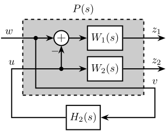
Fig 5: Magnitude of a weighting function generated using the proposed formula
  \setlength\fwidth{6.5cm}
  \setlength\fheight{3.5cm}

  \begin{tikzpicture}
    \begin{axis}[%
      width=1.0\fwidth,
      height=1.0\fheight,
      at={(0.0\fwidth, 0.0\fheight)},
      scale only axis,
      xmode=log,
      xmin=0.1,
      xmax=100,
      xtick={0.1,1,10, 100},
      xminorticks=true,
      ymode=log,
      ymin=0.0005,
      ymax=20,
      ytick={0.001, 0.01, 0.1, 1, 10},
      yminorticks=true,
      ylabel={Magnitude},
      xlabel={Frequency [Hz]},
      xminorgrids,
      yminorgrids,
      ]

      \addplot [color=black, line width=1.5pt, forget plot]
      table [x=freqs, y=ampl, col sep=comma] {/home/thomas/Cloud/thesis/papers/dehaeze19_desig_compl_filte/matlab/matweight_formula.csv};

      \addplot [color=black, dashed, line width=1.5pt]
      table[row sep=crcr]{%
        1     10\\
        100   10\\
      };
      \addplot [color=black, dashed, line width=1.5pt]
      table[row sep=crcr]{%
        0.1  0.001\\
        3    0.001\\
      };

      \addplot [color=black, line width=1.5pt]
      table[row sep=crcr]{%
        0.1  1\\
        100  1\\
      };

      \addplot [color=black, dashed, line width=1.5pt]
      table[row sep=crcr]{%
        10  2\\
        10  1\\
      };

      \node[below] at (2, 10) {$G_\infty$};
      \node[above] at (2, 0.001) {$G_0$};

      \node[branch] at (10, 2){};
      \draw[dashed, line cap=round] (7, 2) -- (20, 2) node[right]{$G_c$};
      \draw[dashed, line cap=round] (10, 2) -- (10, 1) node[below]{$\omega_c$};

      \node[right] at (3, 0.1) {$+n$};

    \end{axis}
  \end{tikzpicture}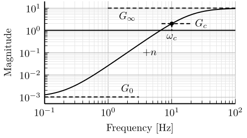
Fig 6: Frequency response of the weighting functions and complementary filters obtained using $\mathcal{H}_\infty$ synthesis
  \setlength\fwidth{6.5cm}
  \setlength\fheight{6cm}

  \begin{tikzpicture}
    \begin{axis}[%
      width=1.0\fwidth,
      height=0.5\fheight,
      at={(0.0\fwidth, 0.47\fheight)},
      scale only axis,
      xmode=log,
      xmin=0.1,
      xmax=1000,
      xtick={0.1, 1, 10, 100, 1000},
      xticklabels={{}},
      xminorticks=true,
      ymode=log,
      ymin=0.0005,
      ymax=20,
      ytick={0.001, 0.01, 0.1, 1, 10},
      yminorticks=true,
      ylabel={Magnitude},
      xminorgrids,
      yminorgrids,
      ]
      \addplot [color=mycolor1, line width=1.5pt, forget plot]
      table [x=freqs, y=H1, col sep=comma] {/home/thomas/Cloud/thesis/papers/dehaeze19_desig_compl_filte/matlab/mathinf_filters_results.csv};

      \addplot [color=mycolor2, line width=1.5pt, forget plot]
      table [x=freqs, y=H2, col sep=comma] {/home/thomas/Cloud/thesis/papers/dehaeze19_desig_compl_filte/matlab/mathinf_filters_results.csv};

      \addplot [color=mycolor1, dashed, line width=1.5pt, forget plot]
      table [x=freqs, y=W1, col sep=comma] {/home/thomas/Cloud/thesis/papers/dehaeze19_desig_compl_filte/matlab/mathinf_weights.csv};

      \addplot [color=mycolor2, dashed, line width=1.5pt, forget plot]
      table [x=freqs, y=W2, col sep=comma] {/home/thomas/Cloud/thesis/papers/dehaeze19_desig_compl_filte/matlab/mathinf_weights.csv};
    \end{axis}

    \begin{axis}[%
      width=1.0\fwidth,
      height=0.45\fheight,
      at={(0.0\fwidth, 0.0\fheight)},
      scale only axis,
      xmode=log,
      xmin=0.1,
      xmax=1000,
      xtick={0.1, 1, 10, 100, 1000},
      xminorticks=true,
      xlabel={Frequency [Hz]},
      ymin=-200,
      ymax=200,
      ytick={-180,  -90,    0,   90,  180},
      ylabel={Phase [deg]},
      xminorgrids,
      legend style={at={(1,1.1)}, outer sep=2pt , anchor=north east, legend cell align=left, align=left, draw=black, nodes={scale=0.7, transform shape}},
      ]
      \addlegendimage{color=mycolor1, dashed, line width=1.5pt}
      \addlegendentry{$W_1^{-1}$};
      \addlegendimage{color=mycolor2, dashed, line width=1.5pt}
      \addlegendentry{$W_2^{-1}$};
      \addplot [color=mycolor1, line width=1.5pt]
      table [x=freqs, y=H1p, col sep=comma] {/home/thomas/Cloud/thesis/papers/dehaeze19_desig_compl_filte/matlab/mathinf_filters_results.csv};
      \addlegendentry{$H_1$};
      \addplot [color=mycolor2, line width=1.5pt]
      table [x=freqs, y=H2p, col sep=comma] {/home/thomas/Cloud/thesis/papers/dehaeze19_desig_compl_filte/matlab/mathinf_filters_results.csv};
      \addlegendentry{$H_2$};
    \end{axis}
  \end{tikzpicture}
Fig 7: Architecture for $\mathcal{H}_\infty$ synthesis of three complementary filters
  \begin{tikzpicture}
     \node[block={5.0cm}{3.5cm}, fill=black!20!white, dashed] (P) {};
     \node[above] at (P.north) {$P(s)$};

     \coordinate[] (inputw)  at ($(P.south west)!0.8!(P.north west) + (-0.7, 0)$);
     \coordinate[] (inputu)  at ($(P.south west)!0.4!(P.north west) + (-0.7, 0)$);

     \coordinate[] (output1) at ($(P.south east)!0.8!(P.north east)  + (0.7, 0)$);
     \coordinate[] (output2) at ($(P.south east)!0.55!(P.north east) + (0.7, 0)$);
     \coordinate[] (output3) at ($(P.south east)!0.3!(P.north east)  + (0.7, 0)$);
     \coordinate[] (outputv) at ($(P.south east)!0.1!(P.north east)  + (0.7, 0)$);

     \node[block, left=1.4 of output1] (W1){$W_1(s)$};
     \node[block, left=1.4 of output2] (W2){$W_2(s)$};
     \node[block, left=1.4 of output3] (W3){$W_3(s)$};
     \node[addb={+}{}{}{}{-}, left=of W1] (sub1) {};
     \node[addb={+}{}{}{}{-}, left=of sub1] (sub2) {};

     \node[block, below=0.3 of P] (H) {$\begin{bmatrix}H_2(s) \\ H_3(s)\end{bmatrix}$};

     \draw[->] (inputw) node[above right](w){$w$} -- (sub2.west);
     \draw[->] (W3-|sub1)node[branch]{} -- (sub1.south);
     \draw[->] (W2-|sub2)node[branch]{} -- (sub2.south);
     \draw[->] ($(sub2.west)+(-0.5, 0)$) node[branch]{} |- (outputv) |- (H.east);
     \draw[->] ($(H.south west)!0.7!(H.north west)$) -| (inputu|-W2) -- (W2.west);
     \draw[->] ($(H.south west)!0.3!(H.north west)$) -| ($(inputu|-W3)+(0.4, 0)$) -- (W3.west);

     \draw[->] (sub2.east) -- (sub1.west);
     \draw[->] (sub1.east) -- (W1.west);
     \draw[->] (W1.east) -- (output1)node[above left](z){$z_1$};
     \draw[->] (W2.east) -- (output2)node[above left]{$z_2$};
     \draw[->] (W3.east) -- (output3)node[above left]{$z_3$};
     \node[above] at (W2-|w){$u_1$};
     \node[above] at (W3-|w){$u_2$};
     \node[above] at (outputv-|z){$v$};
  \end{tikzpicture}
Fig 8: Frequency response of the weighting functions and three complementary filters obtained using $\mathcal{H}_\infty$ synthesis
  \setlength\fwidth{6.5cm}
  \setlength\fheight{6cm}

  \begin{tikzpicture}
    \begin{axis}[%
      width=1.0\fwidth,
      height=0.55\fheight,
      at={(0.0\fwidth, 0.42\fheight)},
      scale only axis,
      xmode=log,
      xmin=0.1,
      xmax=100,
      xticklabels={{}},
      xminorticks=true,
      ymode=log,
      ymin=0.0005,
      ymax=20,
      ytick={0.001, 0.01, 0.1, 1, 10},
      yminorticks=true,
      ylabel={Magnitude},
      xminorgrids,
      yminorgrids,
      legend columns=2,
      legend style={
        /tikz/column 2/.style={
          column sep=5pt,
        },
        at={(1,0)}, outer sep=2pt , anchor=south east, legend cell align=left, align=left, draw=black, nodes={scale=0.7, transform shape}
      },
      ]
      \addplot [color=mycolor1, dashed, line width=1.5pt]
      table [x=freqs, y=W1, col sep=comma] {/home/thomas/Cloud/thesis/papers/dehaeze19_desig_compl_filte/matlab/mathinf_three_weights.csv};
      \addlegendentry{${W_1}^{-1}$};
      \addplot [color=mycolor1, line width=1.5pt]
      table [x=freqs, y=H1, col sep=comma] {/home/thomas/Cloud/thesis/papers/dehaeze19_desig_compl_filte/matlab/mathinf_three_results.csv};
      \addlegendentry{$H_1$};


      \addplot [color=mycolor2, dashed, line width=1.5pt]
      table [x=freqs, y=W2, col sep=comma] {/home/thomas/Cloud/thesis/papers/dehaeze19_desig_compl_filte/matlab/mathinf_three_weights.csv};
      \addlegendentry{${W_2}^{-1}$};
      \addplot [color=mycolor2, line width=1.5pt]
      table [x=freqs, y=H2, col sep=comma] {/home/thomas/Cloud/thesis/papers/dehaeze19_desig_compl_filte/matlab/mathinf_three_results.csv};
      \addlegendentry{$H_2$};

      \addplot [color=mycolor3, dashed, line width=1.5pt]
      table [x=freqs, y=W3, col sep=comma] {/home/thomas/Cloud/thesis/papers/dehaeze19_desig_compl_filte/matlab/mathinf_three_weights.csv};
      \addlegendentry{${W_3}^{-1}$};
      \addplot [color=mycolor3, line width=1.5pt]
      table [x=freqs, y=H3, col sep=comma] {/home/thomas/Cloud/thesis/papers/dehaeze19_desig_compl_filte/matlab/mathinf_three_results.csv};
      \addlegendentry{$H_3$};
    \end{axis}

    \begin{axis}[%
      width=1.0\fwidth,
      height=0.4\fheight,
      at={(0.0\fwidth, 0.0\fheight)},
      scale only axis,
      xmode=log,
      xmin=0.1,
      xmax=100,
      xminorticks=true,
      xlabel={Frequency [Hz]},
      ymin=-240,
      ymax=240,
      ytick={-180,  -90,    0,   90,  180},
      ylabel={Phase [deg]},
      xminorgrids,
      ]

      \addplot [color=mycolor1, line width=1.5pt]
      table [x=freqs, y=H1p, col sep=comma] {/home/thomas/Cloud/thesis/papers/dehaeze19_desig_compl_filte/matlab/mathinf_three_results.csv};

      \addplot [color=mycolor2, line width=1.5pt]
      table [x=freqs, y=H2p, col sep=comma] {/home/thomas/Cloud/thesis/papers/dehaeze19_desig_compl_filte/matlab/mathinf_three_results.csv};

      \addplot [color=mycolor3, line width=1.5pt]
      table [x=freqs, y=H3p, col sep=comma] {/home/thomas/Cloud/thesis/papers/dehaeze19_desig_compl_filte/matlab/mathinf_three_results.csv};
    \end{axis}
  \end{tikzpicture}
Fig 9: Specifications and weighting functions magnitude used for $\mathcal{H}_\infty$ synthesis
  \setlength\fwidth{6.5cm}
  \setlength\fheight{3.2cm}

  \begin{tikzpicture}
    \begin{axis}[%
      width=1.0\fwidth,
      height=1.0\fheight,
      at={(0.0\fwidth, 0.0\fheight)},
      scale only axis,
      separate axis lines,
      every outer x axis line/.append style={black},
      every x tick label/.append style={font=\color{black}},
      every x tick/.append style={black},
      xmode=log,
      xmin=0.001,
      xmax=1,
      xminorticks=true,
      xlabel={Frequency [Hz]},
      every outer y axis line/.append style={black},
      every y tick label/.append style={font=\color{black}},
      every y tick/.append style={black},
      ymode=log,
      ymin=0.005,
      ymax=20,
      yminorticks=true,
      ylabel={Magnitude},
      axis background/.style={fill=white},
      xmajorgrids,
      xminorgrids,
      ymajorgrids,
      yminorgrids,
      legend style={at={(0,1)}, outer sep=2pt, anchor=north west, legend cell align=left, align=left, draw=black, nodes={scale=0.7, transform shape}}
      ]

      \addplot [color=mycolor1, line width=1.5pt]
        table [x=freqs, y=wHm, col sep=comma] {/home/thomas/Cloud/thesis/papers/dehaeze19_desig_compl_filte/matlab/matligo_weights.csv};
      \addlegendentry{$|w_H|^{-1}$}

      \addplot [color=mycolor2, line width=1.5pt]
        table [x=freqs, y=wLm, col sep=comma] {/home/thomas/Cloud/thesis/papers/dehaeze19_desig_compl_filte/matlab/matligo_weights.csv};
      \addlegendentry{$|w_L|^{-1}$}

      \addplot [color=black, dotted, line width=1.5pt]
      table[row sep=crcr]{%
        0.0005	0.008\\
        0.008   0.008\\
      };
      \addlegendentry{Specifications}

      \addplot [color=black, dotted, line width=1.5pt, forget plot]
      table[row sep=crcr]{%
        0.008	0.008\\
        0.04	1\\
      };
      \addplot [color=black, dotted, line width=1.5pt, forget plot]
      table[row sep=crcr]{%
        0.04  3\\
        0.1   3\\
      };
      \addplot [color=black, dotted, line width=1.5pt]
      table[row sep=crcr]{%
        0.1	0.045\\
        2   0.045\\
      };
    \end{axis}
  \end{tikzpicture}
Fig 10: Comparison of the FIR filters (solid) with the filters obtained with $\mathcal{H}_\infty$ synthesis (dashed)
  \setlength\fwidth{6.5cm}
  \setlength\fheight{6.8cm}

  \begin{tikzpicture}
    \begin{axis}[%
      width=1.0\fwidth,
      height=0.60\fheight,
      at={(0.0\fwidth, 0.32\fheight)},
      scale only axis,
      xmode=log,
      xmin=0.001,
      xmax=1,
      xtick={0.001,0.01,0.1,1},
      xticklabels={{}},
      xminorticks=true,
      ymode=log,
      ymin=0.002,
      ymax=5,
      ytick={0.001, 0.01, 0.1, 1, 10},
      yminorticks=true,
      ylabel={Magnitude},
      xminorgrids,
      yminorgrids,
      legend style={at={(1,0)}, outer sep=2pt, anchor=south east, legend cell align=left, align=left, draw=black, nodes={scale=0.7, transform shape}}
      ]
      \addplot [color=mycolor1, line width=1.5pt]
        table [x=freqs, y=Hhm, col sep=comma] {/home/thomas/Cloud/thesis/papers/dehaeze19_desig_compl_filte/matlab/matcomp_ligo_hinf.csv};
      \addlegendentry{$H_H(s)$ - $\mathcal{H}_\infty$}
      \addplot [color=mycolor1, dashed, line width=1.5pt]
        table [x=freqs, y=Hhm, col sep=comma] {/home/thomas/Cloud/thesis/papers/dehaeze19_desig_compl_filte/matlab/matcomp_ligo_fir.csv};
      \addlegendentry{$H_H(s)$ - FIR}
      \addplot [color=mycolor2, line width=1.5pt]
        table [x=freqs, y=Hlm, col sep=comma] {/home/thomas/Cloud/thesis/papers/dehaeze19_desig_compl_filte/matlab/matcomp_ligo_hinf.csv};
      \addlegendentry{$H_L(s)$ - $\mathcal{H}_\infty$}
      \addplot [color=mycolor2, dashed, line width=1.5pt]
        table [x=freqs, y=Hlm, col sep=comma] {/home/thomas/Cloud/thesis/papers/dehaeze19_desig_compl_filte/matlab/matcomp_ligo_fir.csv};
      \addlegendentry{$H_L(s)$ - FIR}
    \end{axis}

    \begin{axis}[%
      width=1.0\fwidth,
      height=0.3\fheight,
      at={(0.0\fwidth, 0.0\fheight)},
      scale only axis,
      xmode=log,
      xmin=0.001,
      xmax=1,
      xtick={0.001,  0.01,   0.1,     1},
      xminorticks=true,
      xlabel={Frequency [Hz]},
      ymin=-180,
      ymax=180,
      ytick={-180,  -90,    0,   90,  180},
      ylabel={Phase [deg]},
      xminorgrids,
      ]
      \addplot [color=mycolor1, line width=1.5pt, forget plot]
        table [x=freqs, y=Hhp, col sep=comma] {/home/thomas/Cloud/thesis/papers/dehaeze19_desig_compl_filte/matlab/matcomp_ligo_hinf.csv};
      \addplot [color=mycolor1, dashed, line width=1.5pt, forget plot]
        table [x=freqs, y=Hhp, col sep=comma] {/home/thomas/Cloud/thesis/papers/dehaeze19_desig_compl_filte/matlab/matcomp_ligo_fir.csv};
      \addplot [color=mycolor2, line width=1.5pt, forget plot]
        table [x=freqs, y=Hlp, col sep=comma] {/home/thomas/Cloud/thesis/papers/dehaeze19_desig_compl_filte/matlab/matcomp_ligo_hinf.csv};
      \addplot [color=mycolor2, dashed, line width=1.5pt, forget plot]
        table [x=freqs, y=Hlp, col sep=comma] {/home/thomas/Cloud/thesis/papers/dehaeze19_desig_compl_filte/matlab/matcomp_ligo_fir.csv};
    \end{axis}
  \end{tikzpicture}