10 KiB
Encoder Renishaw Vionic - Test Bench
This report is also available as a pdf.
Introduction ignore
You can find below the document of:
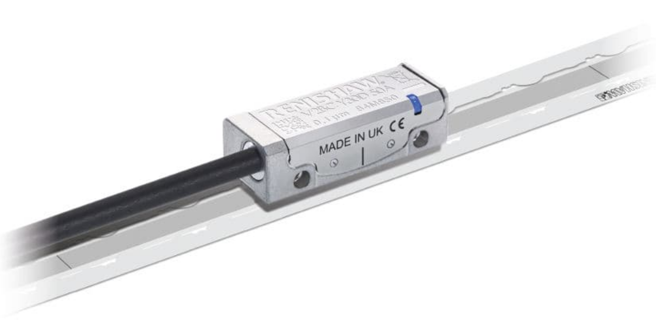
We would like to characterize the encoder measurement system.
In particular, we would like to measure:
- Power Spectral Density of the measurement noise
- Bandwidth of the sensor
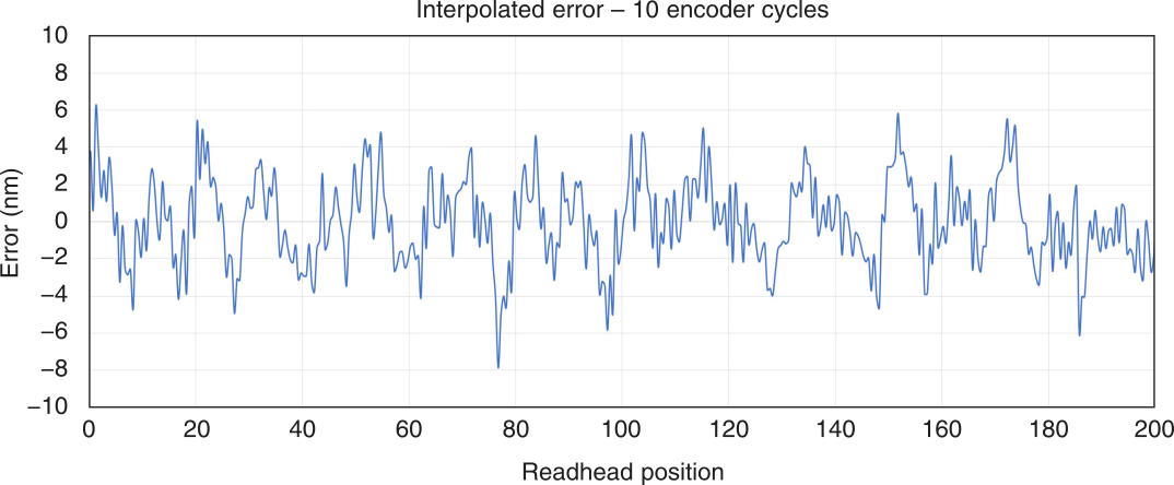
- Linearity of the sensor
Encoder Model
The Encoder is characterized by its dynamics $G_m(s)$ from the "true" displacement $y$ to measured displacement $y_m$. Ideally, this dynamics is constant over a wide frequency band with very small phase drop.
It is also characterized by its measurement noise $n$ that can be described by its Power Spectral Density (PSD).
The model of the encoder is shown in Figure fig:encoder-model-schematic.
  \begin{tikzpicture}
    \node[block] (G) at (0,0){$G_m(s)$};
    \node[addb, left=0.8 of G] (add){};

    \draw[<-] (add.west) -- ++(-1.0, 0) node[above right]{$y$};
    \draw[->] (add.east) -- (G.west);
    \draw[->] (G.east) -- ++(1.0, 0) node[above left]{$y_m$};
    \draw[<-] (add.north) -- ++(0, 0.6) node[below right](n){$n$};

    \begin{scope}[on background layer]
      \node[fit={(add.west|-G.south) (n.north-|G.east)}, inner sep=8pt, draw, dashed, fill=black!20!white] (P) {};
      \node[below left] at (P.north east) {Encoder};
    \end{scope}
  \end{tikzpicture}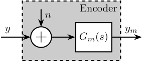
We can also use a transfer function $G_n(s)$ to shape a noise $\tilde{n}$ with unity ASD as shown in Figure fig:vionic_expected_noise.
  \begin{tikzpicture}
    \node[block] (G) at (0,0){$G_m(s)$};
    \node[addb, left=0.8 of G] (add){};
    \node[block, above=0.5 of add] (Gn) {$G_n(s)$};

    \draw[<-] (add.west) -- ++(-1.0, 0) node[above right]{$y$};
    \draw[->] (add.east) -- (G.west);
    \draw[->] (G.east) -- ++(1.0, 0) node[above left]{$y_m$};
    \draw[->] (Gn.south) -- (add.north) node[above right]{$n$};
    \draw[<-] (Gn.north) -- ++(0, 0.6) node[below right](n){$\tilde{n}$};

    \begin{scope}[on background layer]
      \node[fit={(Gn.west|-G.south) (n.north-|G.east)}, inner sep=8pt, draw, dashed, fill=black!20!white] (P) {};
      \node[below left] at (P.north east) {Encoder};
    \end{scope}
  \end{tikzpicture}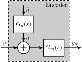
| Characteristics | Manual | Specifications |
|---|---|---|
| Range | Ruler length | > 200 [um] |
| Resolution | 2.5 [nm] | < 50 [nm rms] |
| Sub-Divisional Error | $< \pm 15\,nm$ | |
| Bandwidth | To be checked | > 5 [kHz] |
Noise Measurement
<<sec:noise_measurement>>
Test Bench
To measure the noise $n$ of the encoder, one can rigidly fix the head and the ruler together such that no motion should be measured. Then, the measured signal $y_m$ corresponds to the noise $n$.
Results
First we load the data.
load('noise_meas_100s_20kHz.mat', 't', 'x');
x = x - mean(x);
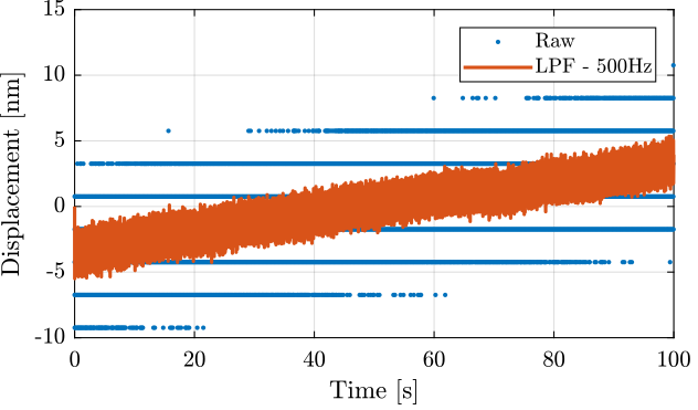
The time domain data are shown in Figure fig:vionic_noise_time.
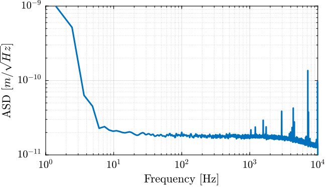
 The amplitude spectral density is computed and shown in Figure fig:vionic_noise_asd.
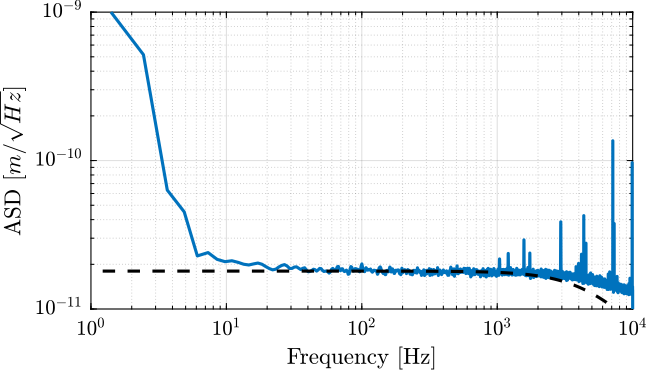
Let's create a transfer function that approximate the measured noise of the encoder.
Gn_e = 1.8e-11/(1 + s/2/pi/5e3);The amplitude of the transfer function and the measured ASD are shown in Figure fig:vionic_noise_asd_model.
Linearity Measurement
<<sec:linearity_measurement>>
Test Bench
In order to measure the linearity, we have to compare the measured displacement with a reference sensor with a known linearity. An interferometer or capacitive sensor should work fine. An actuator should also be there so impose a displacement.
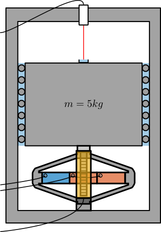
One idea is to use the test-bench shown in Figure fig:test_bench_encoder_calibration.
The APA300ML is used to excite the mass in a broad bandwidth. The motion is measured at the same time by the Vionic Encoder and by an interferometer (most likely an Attocube).
As the interferometer has a very large bandwidth, we should be able to estimate the bandwidth of the encoder if it is less than the Nyquist frequency that can be around 10kHz.
Results
Dynamical Measurement
<<sec:dynamical_measurement>>