20 KiB
Encoder Renishaw Vionic - Test Bench
This report is also available as a pdf.
Introduction ignore
You can find below the documentation of:
In this document, we wish to characterize the performances of the encoder measurement system. In particular, we would like to measure:
- the measurement noise
- the linearity of the sensor
- the bandwidth of the sensor
This document is structured as follow:
- Section sec:vionic_expected_performances: the expected performance of the Vionic encoder system are described
- Section sec:encoder_model: a simple model of the encoder is developed
- Section sec:noise_measurement: the noise of the encoder is measured and a model of the noise is identified
- Section sec:linearity_measurement: the linearity of the sensor is estimated
Expected Performances
<<sec:vionic_expected_performances>>
The Vionic encoder is shown in Figure fig:encoder_vionic.
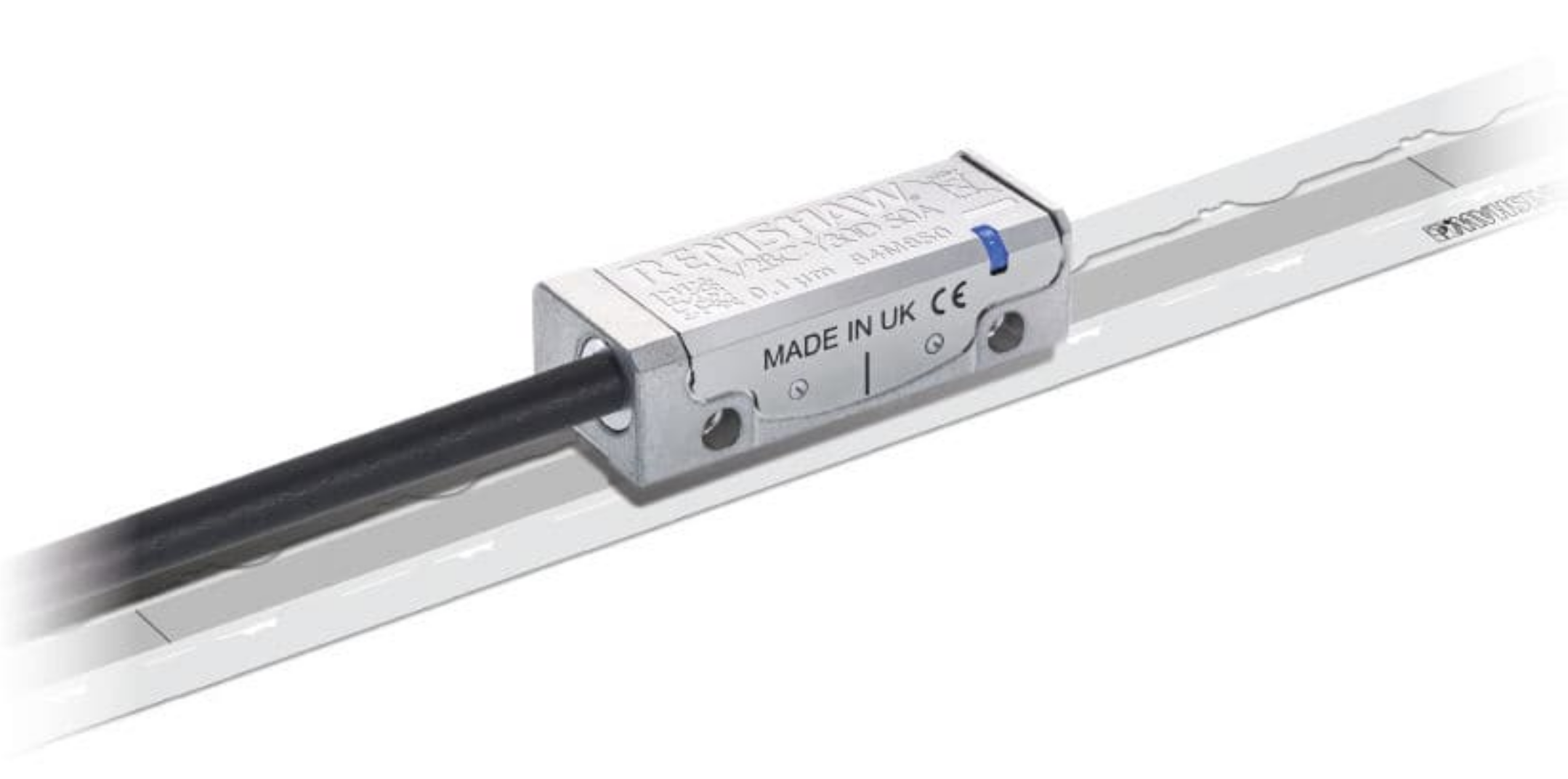
From the Renishaw website:
The VIONiC encoder features the third generation of Renishaw's unique filtering optics that average the contributions from many scale periods and effectively filter out non-periodic features such as dirt. The nominally square-wave scale pattern is also filtered to leave a pure sinusoidal fringe field at the detector. Here, a multiple finger structure is employed, fine enough to produce photocurrents in the form of four symmetrically phased signals. These are combined to remove DC components and produce sine and cosine signal outputs with high spectral purity and low offset while maintaining bandwidth to beyond 500 kHz.
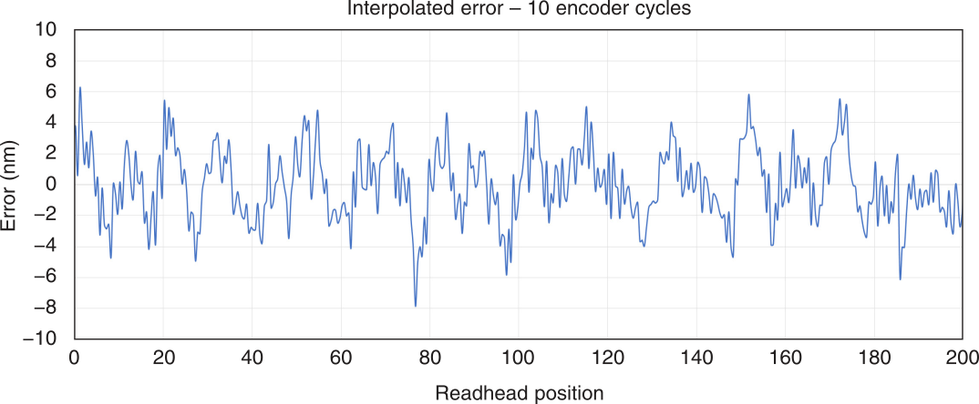
Fully integrated advanced dynamic signal conditioning, Auto Gain , Auto Balance and Auto Offset Controls combine to ensure ultra-low Sub-Divisional Error (SDE) of typically $<\pm 15\, nm$.
This evolution of filtering optics, combined with carefully-selected electronics, provide incremental signals with wide bandwidth achieving a maximum speed of 12 m/s with the lowest positional jitter (noise) of any encoder in its class. Interpolation is within the readhead, with fine resolution versions being further augmented by additional noise-reducing electronics to achieve jitter of just 1.6 nm RMS.
The expected interpolation errors (non-linearity) is shown in Figure fig:vionic_expected_noise.
The characteristics as advertise in the manual as well as our specifications are shown in Table tab:vionic_characteristics.
| Characteristics | Manual | Specification |
|---|---|---|
| Time Delay | < 10 ns | < 0.5 ms |
| Bandwidth | > 500 kHz | > 5 kHz |
| Noise | < 1.6 nm rms | < 50 nm rms |
| Linearity | < +/- 15 nm | |
| Range | Ruler length | > 200 um |
Encoder Model
<<sec:encoder_model>>
The Encoder is characterized by its dynamics $G_m(s)$ from the "true" displacement $y$ to measured displacement $y_m$. Ideally, this dynamics is constant over a wide frequency band with very small phase drop.
It is also characterized by its measurement noise $n$ that can be described by its Power Spectral Density (PSD) $\Gamma_n(\omega)$.
The model of the encoder is shown in Figure fig:encoder-model-schematic.
  \begin{tikzpicture}
    \node[block] (G) at (0,0){$G_m(s)$};
    \node[addb, left=0.8 of G] (add){};

    \draw[<-] (add.west) -- ++(-1.0, 0) node[above right]{$y$};
    \draw[->] (add.east) -- (G.west);
    \draw[->] (G.east) -- ++(1.0, 0) node[above left]{$y_m$};
    \draw[<-] (add.north) -- ++(0, 0.6) node[below right](n){$n$};

    \begin{scope}[on background layer]
      \node[fit={(add.west|-G.south) (n.north-|G.east)}, inner sep=8pt, draw, dashed, fill=black!20!white] (P) {};
      \node[below left] at (P.north east) {Encoder};
    \end{scope}
  \end{tikzpicture}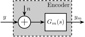
We can also use a transfer function $G_n(s)$ to shape a noise $\tilde{n}$ with unity ASD as shown in Figure fig:vionic_expected_noise.
  \begin{tikzpicture}
    \node[block] (G) at (0,0){$G_m(s)$};
    \node[addb, left=0.8 of G] (add){};
    \node[block, above=0.5 of add] (Gn) {$G_n(s)$};

    \draw[<-] (add.west) -- ++(-1.0, 0) node[above right]{$y$};
    \draw[->] (add.east) -- (G.west);
    \draw[->] (G.east) -- ++(1.0, 0) node[above left]{$y_m$};
    \draw[->] (Gn.south) -- (add.north) node[above right]{$n$};
    \draw[<-] (Gn.north) -- ++(0, 0.6) node[below right](n){$\tilde{n}$};

    \begin{scope}[on background layer]
      \node[fit={(Gn.west|-G.south) (n.north-|G.east)}, inner sep=8pt, draw, dashed, fill=black!20!white] (P) {};
      \node[below left] at (P.north east) {Encoder};
    \end{scope}
  \end{tikzpicture}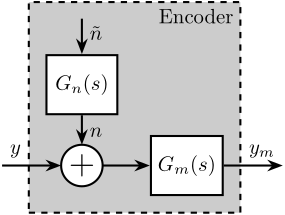
Noise Measurement
<<sec:noise_measurement>>
Introduction ignore
This part is structured as follow:
- Section sec:noise_bench: the measurement bench is described
- Section sec:thermal_drifts: long measurement is performed to estimate the low frequency drifts in the measurement
- Section sec:vionic_noise_time: high frequency measurements are performed to estimate the high frequency noise
- Section sec:noise_asd: the Spectral density of the measurement noise is estimated
- Section sec:vionic_noise_model: finally, the measured noise is modeled
Test Bench
<<sec:noise_bench>>
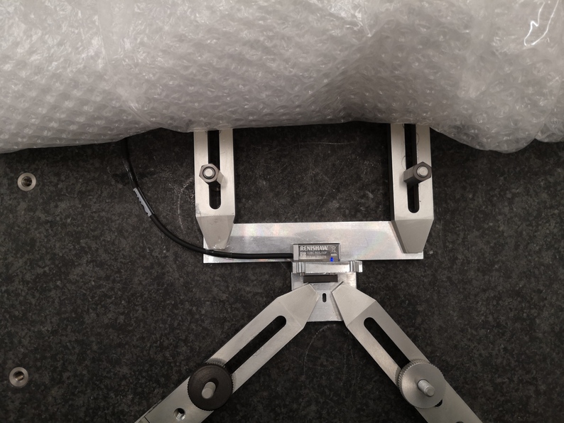
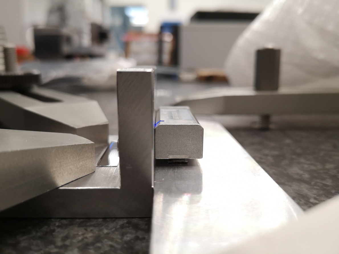
To measure the noise $n$ of the encoder, one can rigidly fix the head and the ruler together such that no motion should be measured. Then, the measured signal $y_m$ corresponds to the noise $n$.
The measurement bench is shown in Figures fig:meas_bench_top_view and fig:meas_bench_side_view. Note that the bench is then covered with a "plastic bubble sheet" in order to keep disturbances as small as possible.
Thermal drifts
<<sec:thermal_drifts>> Measured displacement were recording during approximately 40 hours with a sample frequency of 100Hz. A first order low pass filter with a corner frequency of 1Hz
enc_l = load('mat/noise_meas_40h_100Hz_1.mat', 't', 'x');The measured time domain data are shown in Figure fig:vionic_drifts_time.
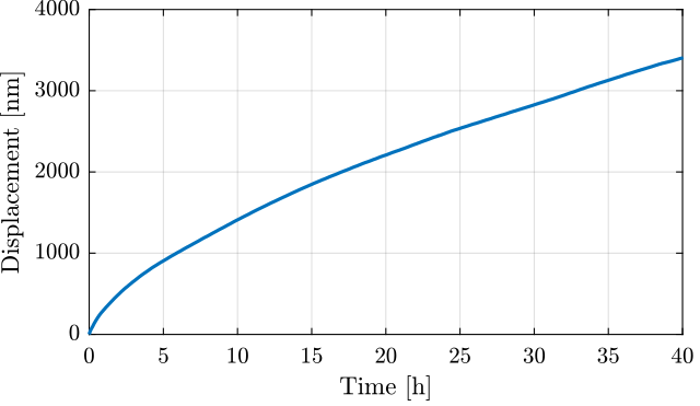
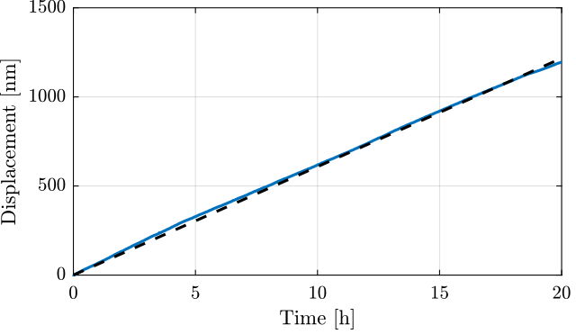
The measured data seems to experience a constant drift after approximately 20 hour. Let's estimate this drift.
The mean drift is approximately 60.9 [nm/hour] or 1.0 [nm/min]
Comparison between the data and the linear fit is shown in Figure fig:vionic_drifts_linear_fit.
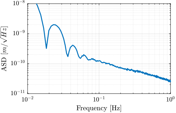
Let's now estimate the Power Spectral Density of the measured displacement. The obtained low frequency ASD is shown in Figure fig:vionic_noise_asd_low_freq.
Time Domain signals
<<sec:vionic_noise_time>>
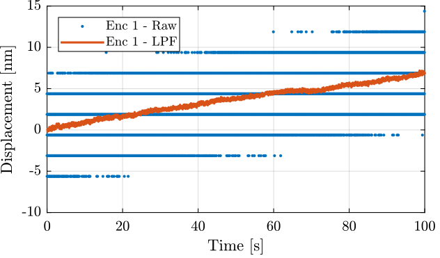
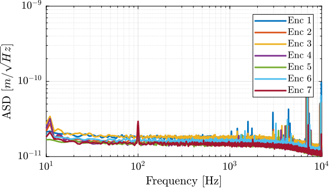
Then, and for all the 7 encoders, we record the measured motion during 100s with a sampling frequency of 20kHz.
The raw measured data as well as the low pass filtered data (using a first order low pass filter with a cut-off at 10Hz) are shown in Figure fig:vionic_noise_raw_lpf.
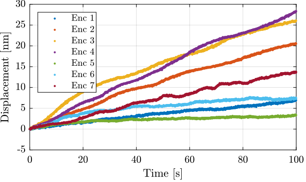
The time domain data for all the encoders are compared in Figure fig:vionic_noise_time.
We can see some drifts that are in the order of few nm to 20nm per minute. As shown in Section sec:thermal_drifts, these drifts should diminish over time down to 1nm/min.
Noise Spectral Density
<<sec:noise_asd>>
The amplitude spectral densities for all the encoder are computed and shown in Figure fig:vionic_noise_asd.
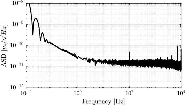
We can combine these measurements with the low frequency noise computed in Section sec:thermal_drifts. The obtained ASD is shown in Figure fig:vionic_noise_asd_combined.
Noise Model
<<sec:vionic_noise_model>>
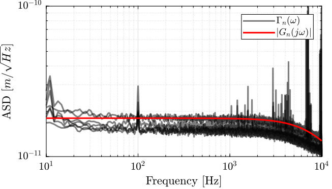
Let's create a transfer function that approximate the measured noise of the encoder.
Gn_e = 1.8e-11/(1 + s/2/pi/1e4);The amplitude of the transfer function and the measured ASD are shown in Figure fig:vionic_noise_asd_model.
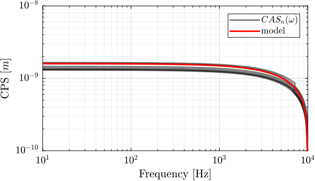
The cumulative amplitude spectrum is now computed and shown in Figure fig:vionic_noise_cas_model.
We can see that the Root Mean Square value of the measurement noise is $\approx 1.6 \, nm$ as advertise in the datasheet.
Linearity Measurement
<<sec:linearity_measurement>>
Test Bench
In order to measure the linearity, we have to compare the measured displacement with a reference sensor with a known linearity. An interferometer or capacitive sensor should work fine. An actuator should also be there so impose a displacement.
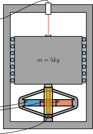
One idea is to use the test-bench shown in Figure fig:test_bench_encoder_calibration.
The APA300ML is used to excite the mass in a broad bandwidth. The motion is measured at the same time by the Vionic Encoder and by an interferometer (most likely an Attocube).
As the interferometer has a very large bandwidth, we should be able to estimate the bandwidth of the encoder if it is less than the Nyquist frequency that can be around 10kHz.