150 KiB
Amplifier Piezoelectric Actuator APA300ML - Test Bench
- Introduction
- Model of an Amplified Piezoelectric Actuator and Sensor
- Geometrical Measurements
- Electrical Measurements
- Stroke measurement
- Stiffness measurement
- Test-Bench Description
- Measurement Procedure
- FRF measurement
- Measurement Results
- Test Bench APA300ML - Simscape Model
- Test Bench Struts - Simscape Model
- Resonance frequencies - APA300ML
- Function
- Bibliography
This report is also available as a pdf.
Introduction ignore
The goal of this test bench is to extract all the important parameters of the Amplified Piezoelectric Actuator APA300ML.
This include:
- Stroke
- Stiffness
- Hysteresis
- Gain from the applied voltage $V_a$ to the generated Force $F_a$
- Gain from the sensor stack strain $\delta L$ to the generated voltage $V_s$
- Dynamical behavior
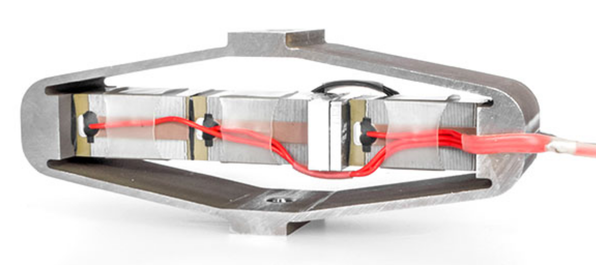
Model of an Amplified Piezoelectric Actuator and Sensor
Consider a schematic of the Amplified Piezoelectric Actuator in Figure fig:apa_model_schematic.
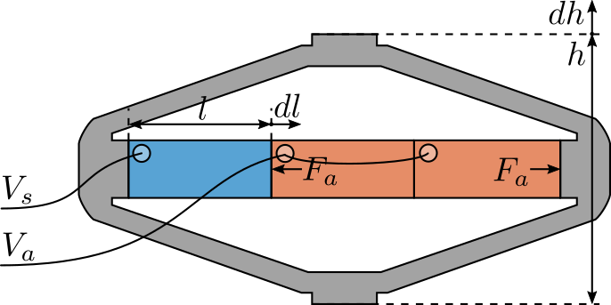
A voltage $V_a$ applied to the actuator stacks will induce an actuator force $F_a$:
\begin{equation} F_a = g_a \cdot V_a \end{equation}A change of length $dl$ of the sensor stack will induce a voltage $V_s$:
\begin{equation} V_s = g_s \cdot dl \end{equation}We wish here to experimental measure $g_a$ and $g_s$.
The block-diagram model of the piezoelectric actuator is then as shown in Figure fig:apa-model-simscape-schematic.
  \begin{tikzpicture}
    \node[block={2.0cm}{2.0cm}, align=center] (model) at (0,0){Simscape\\Model};
    \node[block, left=1.0 of model] (ga){$g_a(s)$};
    \node[block, right=1.0 of model] (gs){$g_s(s)$};

    \draw[<-] (ga.west) -- node[midway, above]{$V_a$} node[midway, below]{$[V]$} ++(-1.0, 0);
    \draw[->] (ga.east) --node[midway, above]{$F_a$} node[midway, below]{$[N]$} (model.west);
    \draw[->] (model.east) --node[midway, above]{$dl$} node[midway, below]{$[m]$} (gs.west);
    \draw[->] (gs.east) -- node[midway, above]{$V_s$} node[midway, below]{$[V]$} ++(1.0, 0);
  \end{tikzpicture}
Geometrical Measurements
Introduction ignore
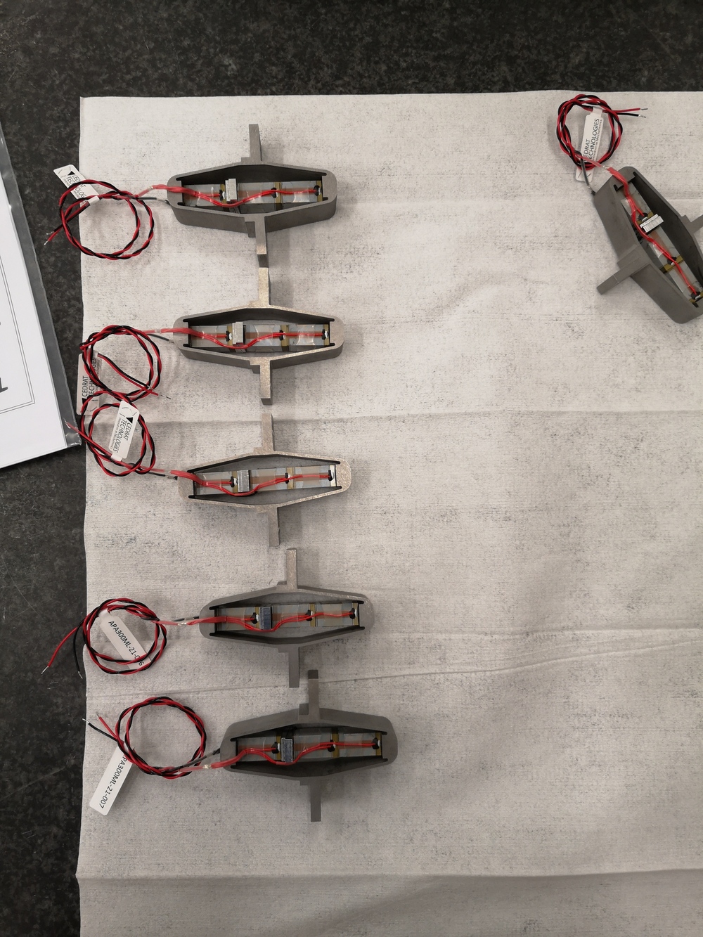
The received APA are shown in Figure fig:received_apa.
Measurement Setup
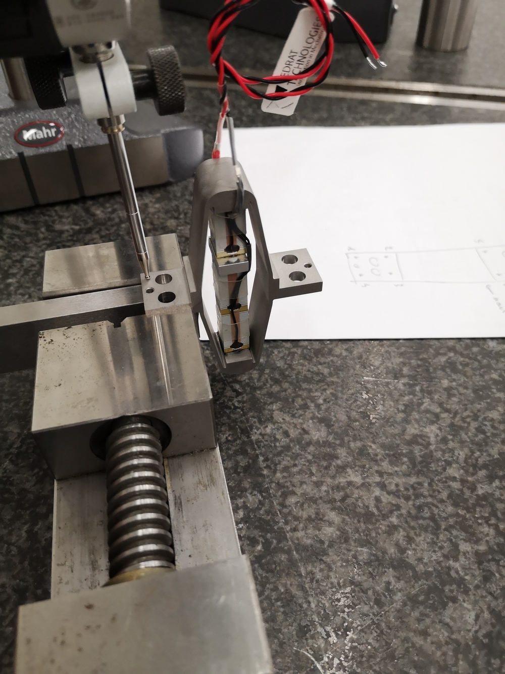
The flatness corresponding to the two interface planes are measured as shown in Figure fig:flatness_meas_setup.
Measurement Results
The height (Z) measurements at the 8 locations (4 points by plane) are defined below.
apa1  = 1e-6*[0, -0.5 , 3.5  , 3.5  , 42   , 45.5, 52.5 , 46];
apa2  = 1e-6*[0, -2.5 , -3   , 0    , -1.5 , 1   , -2   , -4];
apa3  = 1e-6*[0, -1.5 , 15   , 17.5 , 6.5  , 6.5 , 21   , 23];
apa4  = 1e-6*[0, 6.5  , 14.5 , 9    , 16   , 22  , 29.5 , 21];
apa5  = 1e-6*[0, -12.5, 16.5 , 28.5 , -43  , -52 , -22.5, -13.5];
apa6  = 1e-6*[0, -8   , -2   , 5    , -57.5, -62 , -55.5, -52.5];
apa7  = 1e-6*[0, 19.5 , -8   , -29.5, 75   , 97.5, 70   , 48];
apa7b = 1e-6*[0, 9    , -18.5, -30  , 31   , 46.5, 16.5 , 7.5];
apa = {apa1, apa2, apa3, apa4, apa5, apa6, apa7b};
The X/Y Positions of the 8 measurement points are defined below.
W = 20e-3;   % Width [m]
L = 61e-3;   % Length [m]
d = 1e-3;    % Distance from border [m]
l = 15.5e-3; % [m]

pos = [[-L/2 + d; W/2 - d], [-L/2 + l - d; W/2 - d], [-L/2 + l - d; -W/2 + d], [-L/2 + d; -W/2 + d], [L/2 - l + d; W/2 - d], [L/2 - d; W/2 - d], [L/2 - d; -W/2 + d], [L/2 - l + d; -W/2 + d]];
Finally, the flatness is estimated by fitting a plane through the 8 points using the fminsearch command.
apa_d = zeros(1, 7);
for i = 1:7
    fun = @(x)max(abs(([pos; apa{i}]-[0;0;x(1)])'*([x(2:3);1]/norm([x(2:3);1]))));
    x0 = [0;0;0];
    [x, min_d] = fminsearch(fun,x0);
    apa_d(i) = min_d;
end
The obtained flatness are shown in Table tab:flatness_meas.
| Flatness $[\mu m]$ | |
|---|---|
| APA 1 | 8.9 |
| APA 2 | 3.1 |
| APA 3 | 9.1 |
| APA 4 | 3.0 |
| APA 5 | 1.9 |
| APA 6 | 7.1 |
| APA 7 | 18.7 |
Electrical Measurements
The capacitance of the stacks is measure with the LCR-800 Meter (doc)
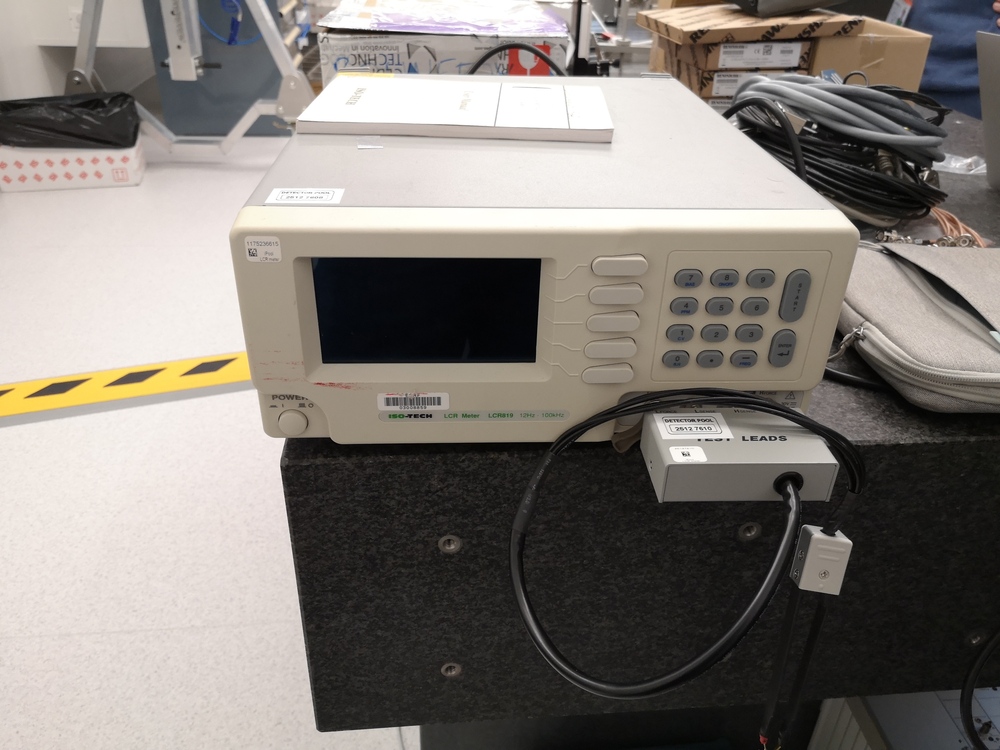
The excitation frequency is set to be 1kHz.
| Sensor Stack | Actuator Stacks | |
|---|---|---|
| APA 1 | 5.10 | 10.03 |
| APA 2 | 4.99 | 9.85 |
| APA 3 | 1.72 | 5.18 |
| APA 4 | 4.94 | 9.82 |
| APA 5 | 4.90 | 9.66 |
| APA 6 | 4.99 | 9.91 |
| APA 7 | 4.85 | 9.85 |
There is clearly a problem with APA300ML number 3
Stroke measurement
Introduction ignore
We here wish to estimate the stroke of the APA.
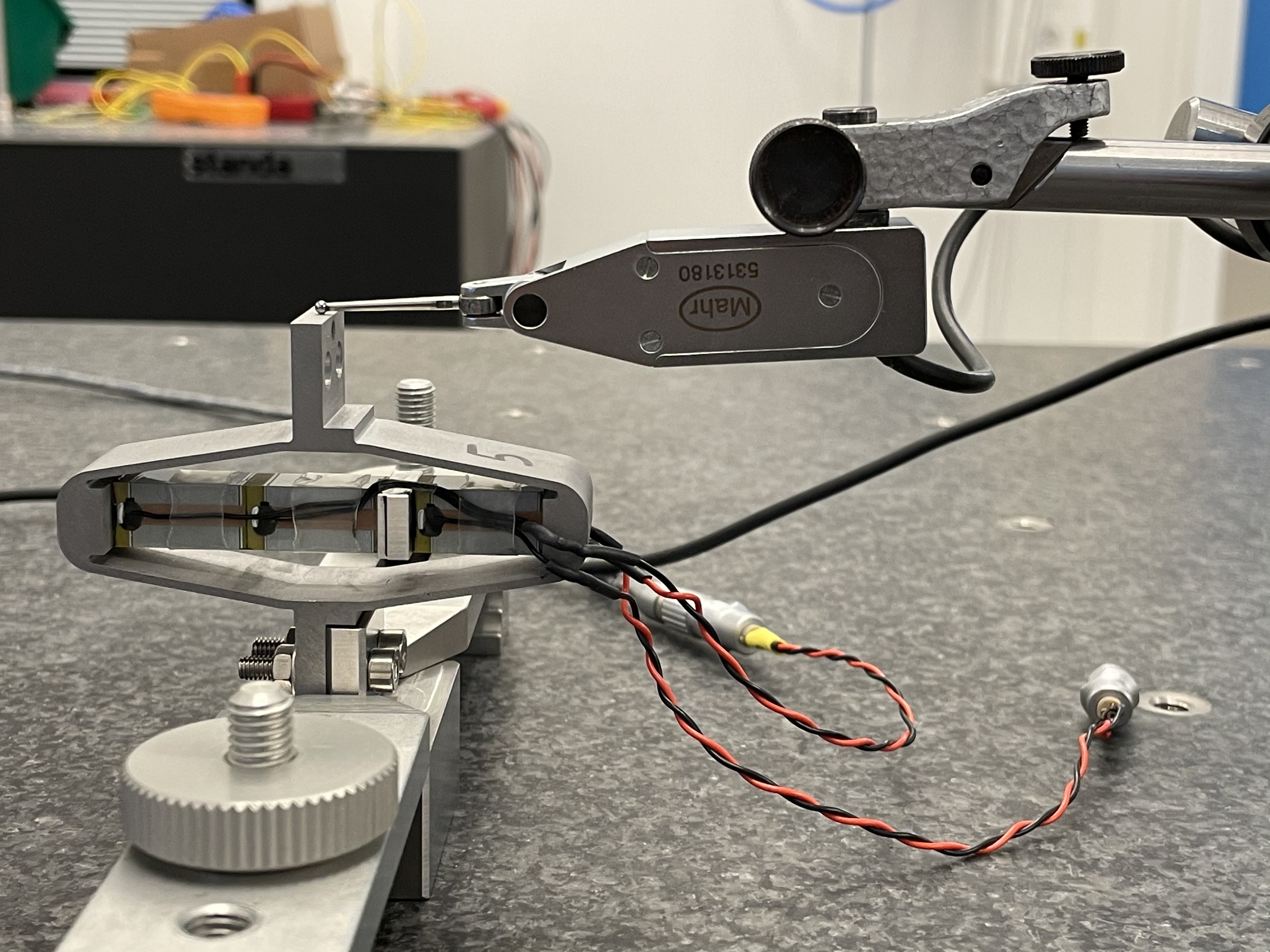
To do so, one side of the APA is fixed, and a displacement probe is located on the other side as shown in Figure fig:stroke_test_bench.
Then, a voltage is applied on either one or two stacks using a DAC and a voltage amplifier.
Here are the documentation of the equipment used for this test bench:
- Voltage Amplifier: PD200 with a gain of 20
- 16bits DAC: IO313 Speedgoat card
- Displacement Probe: Millimar C1216 electronics and Millimar 1318 probe
Voltage applied on one stack
Let's first look at the relation between the voltage applied to one stack to the displacement of the APA as measured by the displacement probe.
The applied voltage is shown in Figure fig:apa_stroke_voltage_time.

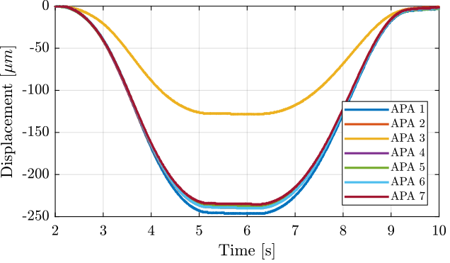
The obtained displacement is shown in Figure fig:apa_stroke_time_1s. The displacement is set to zero at initial time when the voltage applied is -20V.
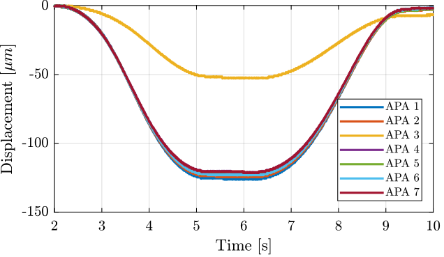
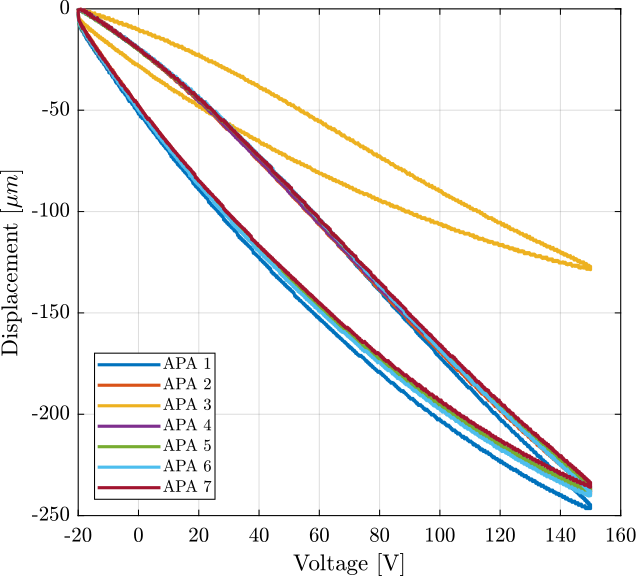
Finally, the displacement is shown as a function of the applied voltage in Figure fig:apa_d_vs_V_1s. We can clearly see that there is a problem with the APA 3. Also, there is a large hysteresis.
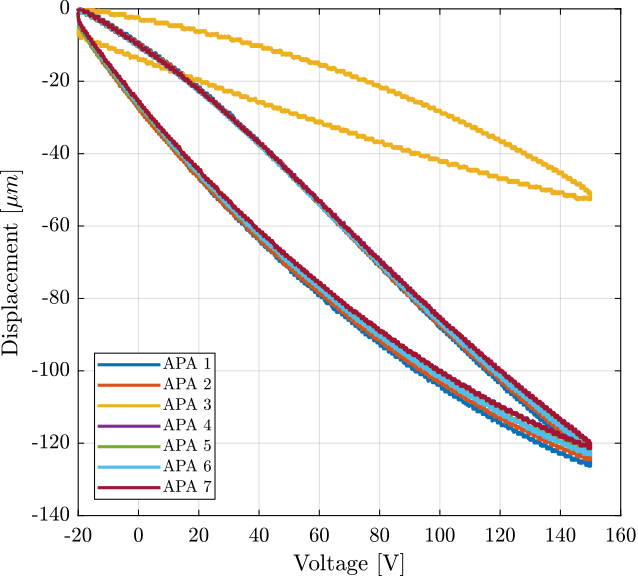
We can clearly see from Figure fig:apa_d_vs_V_1s that there is a problem with the APA number 3.
Voltage applied on two stacks
Now look at the relation between the voltage applied to the two other stacks to the displacement of the APA as measured by the displacement probe.
The obtained displacement is shown in Figure fig:apa_stroke_time_2s. The displacement is set to zero at initial time when the voltage applied is -20V.
Finally, the displacement is shown as a function of the applied voltage in Figure fig:apa_d_vs_V_2s. We can clearly see that there is a problem with the APA 3. Also, there is a large hysteresis.
Voltage applied on all three stacks
Finally, we can combine the two measurements to estimate the relation between the displacement and the voltage applied to the three stacks (Figure fig:apa_d_vs_V_3s).
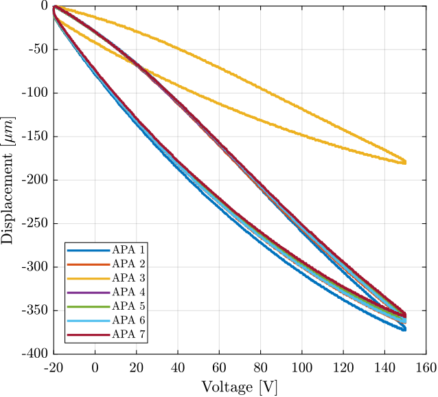
The obtained maximum stroke for all the APA are summarized in Table tab:apa_measured_stroke.
| Stroke $[\mu m]$ | |
|---|---|
| APA 1 | 373.2 |
| APA 2 | 365.5 |
| APA 3 | 181.7 |
| APA 4 | 359.7 |
| APA 5 | 361.5 |
| APA 6 | 363.9 |
| APA 7 | 358.4 |
TODO Stiffness measurement
APA test
load('meas_stiff_apa_1_x.mat', 't', 'F', 'd');figure;
plot(t, F)%% Automatic Zero of the force
F = F - mean(F(t > 0.1 & t < 0.3));
%% Start measurement at t = 0.2 s
d = d(t > 0.2);
F = F(t > 0.2);
t = t(t > 0.2); t = t - t(1);i_l_start = find(F > 0.3, 1, 'first');
[~, i_l_stop] = max(F);F_l = F(i_l_start:i_l_stop);
d_l = d(i_l_start:i_l_stop);fit_l = polyfit(F_l, d_l, 1);
% %% Reset displacement based on fit
% d = d - fit_l(2);
% fit_s(2) = fit_s(2) - fit_l(2);
% fit_l(2) = 0;
% %% Estimated Stroke
% F_max = fit_s(2)/(fit_l(1) - fit_s(1));
% d_max = fit_l(1)*F_max;h^2/fit_l(1)figure;
hold on;
plot(F,d,'k')
plot(F_l, d_l)
plot(F_l, F_l*fit_l(1) + fit_l(2), '--')Test-Bench Description
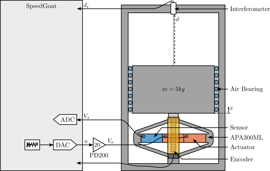
Here are the documentation of the equipment used for this test bench:
- Voltage Amplifier: PD200
- Amplified Piezoelectric Actuator: APA300ML
- DAC/ADC: Speedgoat IO313
- Encoder: Renishaw Vionic and used Ruler
- Interferometer: Attocube IDS3010
Measurement Procedure
<<sec:measurement_procedure>>
Introduction ignore
Stroke Measurement
Using the PD200 amplifier, output a voltage: \[ V_a = 65 + 85 \sin(2\pi \cdot t) \] To have a quasi-static excitation between -20 and 150V.
As the gain of the PD200 amplifier is 20, the DAC output voltage should be: \[ V_{dac}(t) = 3.25 + 4.25\sin(2\pi \cdot t) \]
Verify that the voltage offset of the PD200 is zero!
Measure the output vertical displacement $d$ using the interferometer.
Then, plot $d$ as a function of $V_a$, and perform a linear regression. Conclude on the obtained stroke.
Stiffness Measurement
Add some (known) weight $\delta m g$ on the suspended mass and measure the deflection $\delta d$. This can be tested when the piezoelectric stacks are open-circuit.
As the stiffness will be around $k \approx 10^6 N/m$, an added mass of $m \approx 100g$ will induce a static deflection of $\approx 1\mu m$ which should be large enough for a precise measurement using the interferometer.
Then the obtained stiffness is:
\begin{equation} k = \frac{\delta m g}{\delta d} \end{equation}Hysteresis measurement
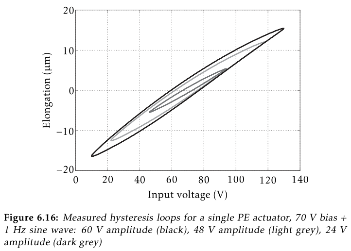
Supply a quasi static sinusoidal excitation $V_a$ at different voltages.
The offset should be 65V, and the sin amplitude can range from 1V up to 85V.
For each excitation amplitude, the vertical displacement $d$ of the mass is measured.
Then, $d$ is plotted as a function of $V_a$ for all the amplitudes.
Piezoelectric Actuator Constant
Using the measurement test-bench, it is rather easy the determine the static gain between the applied voltage $V_a$ to the induced displacement $d$. Use a quasi static (1Hz) excitation signal $V_a$ on the piezoelectric stack and measure the vertical displacement $d$. Perform a linear regression to obtain:
\begin{equation} d = g_{d/V_a} \cdot V_a \end{equation}Using the Simscape model of the APA, it is possible to determine the static gain between the actuator force $F_a$ to the induced displacement $d$:
\begin{equation} d = g_{d/F_a} \cdot F_a \end{equation}From the two gains, it is then easy to determine $g_a$:
\begin{equation} g_a = \frac{F_a}{V_a} = \frac{F_a}{d} \cdot \frac{d}{V_a} = \frac{g_{d/V_a}}{g_{d/F_a}} \end{equation}Piezoelectric Sensor Constant
From a quasi static excitation of the piezoelectric stack, measure the gain from $V_a$ to $V_s$:
\begin{equation} V_s = g_{V_s/V_a} V_a \end{equation}Note here that there is an high pass filter formed by the piezo capacitor and parallel resistor. The excitation frequency should then be in between the cut-off frequency of this high pass filter and the first resonance.
Alternatively, the gain can be computed from the dynamical identification and taking the gain at the wanted frequency.
Using the simscape model, compute the static gain from the actuator force $F_a$ to the strain of the sensor stack $dl$:
\begin{equation} dl = g_{dl/F_a} F_a \end{equation}Then, the static gain from the sensor stack strain $dl$ to the general voltage $V_s$ is:
\begin{equation} g_s = \frac{V_s}{dl} = \frac{V_s}{V_a} \cdot \frac{V_a}{F_a} \cdot \frac{F_a}{dl} = \frac{g_{V_s/V_a}}{g_a \cdot g_{dl/F_a}} \end{equation}Alternatively, we could impose an external force to add strain in the APA that should be equally present in all the 3 stacks and equal to 1/5 of the vertical strain. This external force can be some weight added, or a piezo in parallel.
Capacitance Measurement
Measure the capacitance of the 3 stacks individually using a precise multi-meter.
Dynamical Behavior
Perform a system identification from $V_a$ to the measured displacement $d$ by the interferometer and by the encoder, and to the generated voltage $V_s$.
This can be performed using different excitation signals.
This can also be performed with and without the encoder fixed to the APA.
Compare the results obtained for all 7 APA300ML
Compare all the obtained parameters for all the test APA.
FRF measurement
Introduction ignore
- Schematic of the measurement
| Variable | Unit | Hardware | |
|---|---|---|---|
Va |
Output DAC voltage | [V] | DAC - Ch. 1 => PD200 => APA |
Vs |
Measured stack voltage (ADC) | [V] | APA => ADC - Ch. 1 |
de |
Encoder Measurement | [m] | PEPU Ch. 1 - IO318(1) - Ch. 1 |
da |
Attocube Measurement | [m] | PEPU Ch. 2 - IO318(1) - Ch. 2 |
t |
Time | [s] |
frf_setup.m - Measurement Setup
First is defined the sampling frequency:
%% Simulation configuration
Fs   = 10e3; % Sampling Frequency [Hz]
Ts   = 1/Fs; % Sampling Time [s]
%% Data record configuration
Trec_start = 5; % Start time for Recording [s]
Trec_dur = 100; % Recording Duration [s]Tsim = 2*Trec_start + Trec_dur; % Simulation Time [s]The maximum excitation voltage at resonance is 9Vrms, therefore corresponding to 0.6V of output DAC voltage.
%% Sweep Sine
gc = 0.1;
xi = 0.5;
wn = 2*pi*94.3;

% Notch filter at the resonance of the APA
G_sweep = 0.2*(s^2 + 2*gc*xi*wn*s + wn^2)/(s^2 + 2*xi*wn*s + wn^2);

V_sweep = generateSweepExc('Ts',      Ts, ...
                           'f_start', 10, ...
                           'f_end',   1e3, ...
                           'V_mean',  3.25, ...
                           't_start', Trec_start, ...
                           'exc_duration', Trec_dur, ...
                           'sweep_type',   'log', ...
                           'V_exc', G_sweep*1/(1 + s/2/pi/500));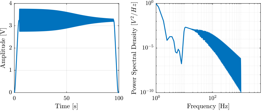
A white noise excitation signal can be very useful in order to obtain a first idea of the plant FRF. The gain can be gradually increased until satisfactory output is obtained.
%% Shaped Noise
V_noise = generateShapedNoise('Ts', 1/Fs, ...
                              'V_mean', 3.25, ...
                              't_start', Trec_start, ...
                              'exc_duration', Trec_dur, ...
                              'smooth_ends', true, ...
                              'V_exc', 0.05/(1 + s/2/pi/10));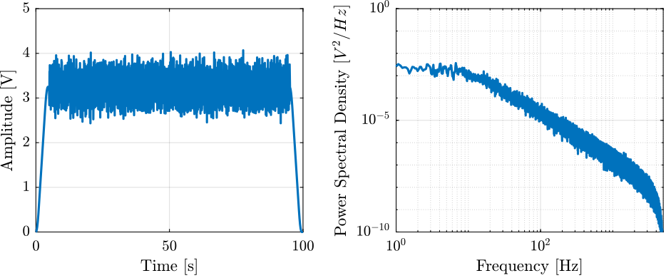
%% Sinus excitation with increasing amplitude
V_sin = generateSinIncreasingAmpl('Ts', 1/Fs, ...
                                    'V_mean', 3.25, ...
                                    'sin_ampls', [0.1, 0.2, 0.4, 1, 2, 4], ...
                                    'sin_period', 1, ...
                                    'sin_num', 5, ...
                                    't_start', 10, ...
                                    'smooth_ends', true);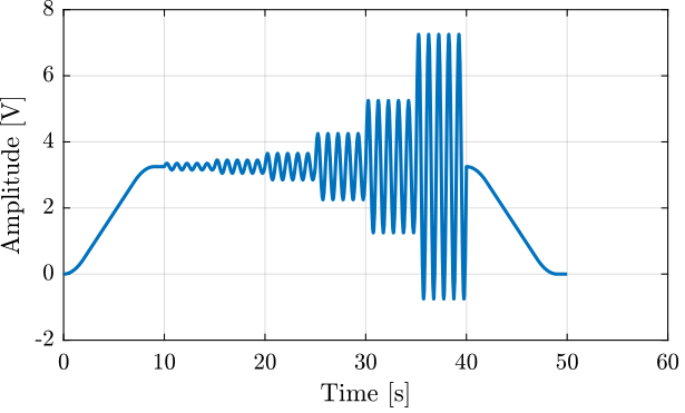
Then, we select the wanted excitation signal.
%% Select the excitation signal
V_exc = timeseries(V_noise(2,:), V_noise(1,:));
%% Save data that will be loaded in the Simulink file
save('./frf_data.mat', 'Fs', 'Ts', 'Tsim', 'Trec_start', 'Trec_dur', 'V_exc');
frf_save.m - Save Data
First, we get data from the Speedgoat:
tg = slrt;

f = SimulinkRealTime.openFTP(tg);
mget(f, 'data/data.dat');
close(f);
And we load the data on the Workspace:
data = SimulinkRealTime.utils.getFileScopeData('data/data.dat').data;

da = data(:, 1); % Excitation Voltage (input of PD200) [V]
de = data(:, 2); % Measured voltage (force sensor) [V]
Vs = data(:, 3); % Measurment displacement (encoder) [m]
Va = data(:, 4); % Measurement displacement (attocube) [m]
t  = data(:, end); % Time [s]
And we save this to a mat file:
apa_number = 1;

save(sprintf('mat/frf_data_%i_huddle.mat', apa_number), 't', 'Va', 'Vs', 'de', 'da');
Measurements on APA 1
Introduction ignore
Measurements are first performed on the APA number 1.
Huddle Test
load(sprintf('frf_data_%i_huddle.mat', 1), 't', 'Va', 'Vs', 'de', 'da');%% Parameter for Spectral analysis
Ts = (t(end) - t(1))/(length(t)-1);
Fs = 1/Ts;
win = hanning(ceil(10*Fs)); % Hannning Windows[phh_da, f] = pwelch(da - mean(da), win, [], [], 1/Ts);
[phh_de, ~] = pwelch(de - mean(de), win, [], [], 1/Ts);
[phh_Vs, ~] = pwelch(Vs - mean(Vs), win, [], [], 1/Ts);First identification with Noise
load(sprintf('mat/frf_data_%i_noise.mat', 1), 't', 'Va', 'Vs', 'da', 'de')[pxx_da, f] = pwelch(da, win, [], [], 1/Ts);
[pxx_de, ~] = pwelch(de, win, [], [], 1/Ts);
[pxx_Vs, ~] = pwelch(Vs, win, [], [], 1/Ts);[G_dvf, f] = tfestimate(Va, de, win, [], [], 1/Ts);
[G_d, ~] = tfestimate(Va, da, win, [], [], 1/Ts);
[G_iff, ~] = tfestimate(Va, Vs, win, [], [], 1/Ts);
[coh_dvf, ~] = mscohere(Va, de, win, [], [], 1/Ts);
[coh_d, ~] = mscohere(Va, da, win, [], [], 1/Ts);
[coh_iff, ~] = mscohere(Va, Vs, win, [], [], 1/Ts);Second identification with Sweep and high frequency noise
load(sprintf('mat/frf_data_%i_sweep.mat', 1), 't', 'Va', 'Vs', 'da', 'de')[pxx_da, f] = pwelch(da, win, [], [], 1/Ts);
[pxx_de, ~] = pwelch(de, win, [], [], 1/Ts);
[pxx_Vs, ~] = pwelch(Vs, win, [], [], 1/Ts);[G_dvf, f] = tfestimate(Va, de, win, [], [], 1/Ts);
[G_d, ~] = tfestimate(Va, da, win, [], [], 1/Ts);
[G_iff, ~] = tfestimate(Va, Vs, win, [], [], 1/Ts);
[coh_dvf, ~] = mscohere(Va, de, win, [], [], 1/Ts);
[coh_d, ~] = mscohere(Va, da, win, [], [], 1/Ts);
[coh_iff, ~] = mscohere(Va, Vs, win, [], [], 1/Ts);load(sprintf('mat/frf_data_%i_noise_high_freq.mat', 1), 't', 'Va', 'Vs', 'da', 'de')[phf_da, f] = pwelch(da, win, [], [], 1/Ts);
[phf_de, ~] = pwelch(de, win, [], [], 1/Ts);
[phf_Vs, ~] = pwelch(Vs, win, [], [], 1/Ts);[cohhf_dvf, ~] = mscohere(Va, de, win, [], [], 1/Ts);
[cohhf_d, ~] = mscohere(Va, da, win, [], [], 1/Ts);
[cohhf_iff, ~] = mscohere(Va, Vs, win, [], [], 1/Ts);
[Ghf_dvf, f] = tfestimate(Va, de, win, [], [], 1/Ts);
[Ghf_d, ~] = tfestimate(Va, da, win, [], [], 1/Ts);
[Ghf_iff, ~] = tfestimate(Va, Vs, win, [], [], 1/Ts);Extract Parameters (Actuator/Sensor constants)
Quasi static gain between $d$ and $V_a$:
g_d_Va = mean(abs(G_dvf(f > 10 & f < 15)));g_d_Va = 1.7e-05 [m/V]
Quasi static gain between $V_s$ and $V_a$:
g_Vs_Va = mean(abs(G_iff(f > 10 & f < 15)));g_Vs_Va = 5.7e-01 [V/V]
Comparison of all the APA
Introduction ignore
Stiffness - Comparison of the APA
In order to estimate the stiffness of the APA, a weight with known mass $m_a$ is added on top of the suspended granite and the deflection $d_e$ is measured using an encoder. The APA stiffness is then:
\begin{equation} k_{\text{apa}} = \frac{m_a g}{d} \end{equation}Here are the number of the APA that have been measured:
apa_nums = [1 2 4 5 6 7 8];The data are loaded.
apa_mass = {};
for i = 1:length(apa_nums)
    apa_mass(i) = {load(sprintf('frf_data_%i_add_mass_closed_circuit.mat', apa_nums(i)), 't', 'de')};
    % The initial displacement is set to zero
    apa_mass{i}.de = apa_mass{i}.de - mean(apa_mass{i}.de(apa_mass{i}.t<11));
end
The raw measurements are shown in Figure fig:apa_meas_k_time. All the APA seems to have similar stiffness except the APA 7 which should have an higher stiffness.
It is however strange that the displacement $d_e$ when the mass is removed is higher for the APA 7 than for the other APA. What could cause that?
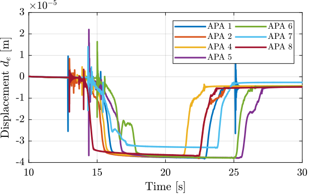
added_mass = 6.4; % Added mass [kg]The stiffnesses are computed for all the APA and are summarized in Table tab:APA_measured_k.
| APA Num | $k [N/\mu m]$ |
|---|---|
| 1 | 1.68 |
| 2 | 1.69 |
| 4 | 1.7 |
| 5 | 1.7 |
| 6 | 1.7 |
| 7 | 1.93 |
| 8 | 1.73 |
The APA300ML manual specifies the nominal stiffness to be $1.8\,[N/\mu m]$ which is very close to what have been measured. Only the APA number 7 is a little bit off.
Stiffness - Effect of connecting the actuator stack to the amplifier and the sensor stack to the ADC
We wish here to see if the stiffness changes when the actuator stacks are not connected to the amplifier and the sensor stacks are not connected to the ADC.
Note here that the resistor in parallel to the sensor stack is present in both cases.
First, the data are loaded.
add_mass_oc = load(sprintf('frf_data_%i_add_mass_open_circuit.mat',   1), 't', 'de');
add_mass_cc = load(sprintf('frf_data_%i_add_mass_closed_circuit.mat', 1), 't', 'de');
And the initial displacement is set to zero.
add_mass_oc.de = add_mass_oc.de - mean(add_mass_oc.de(add_mass_oc.t<11));
add_mass_cc.de = add_mass_cc.de - mean(add_mass_cc.de(add_mass_cc.t<11));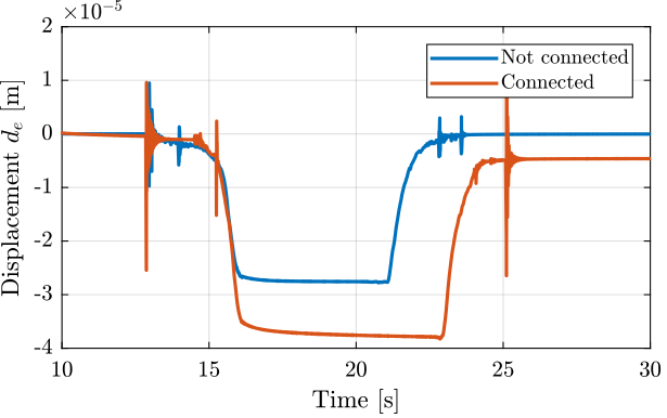
And the stiffness is estimated in both case. The results are shown in Table tab:APA_measured_k_oc_cc.
apa_k_oc = 9.8 * added_mass / (mean(add_mass_oc.de(add_mass_oc.t > 12 & add_mass_oc.t < 12.5)) - mean(add_mass_oc.de(add_mass_oc.t > 20 & add_mass_oc.t < 20.5)));
apa_k_cc = 9.8 * added_mass / (mean(add_mass_cc.de(add_mass_cc.t > 12 & add_mass_cc.t < 12.5)) - mean(add_mass_cc.de(add_mass_cc.t > 20 & add_mass_cc.t < 20.5)));| $k [N/\mu m]$ | |
|---|---|
| Not connected | 2.3 |
| Connected | 1.7 |
Clearly, connecting the actuator stacks to the amplified (basically equivalent as to short circuiting them) lowers the stiffness.
Hysteresis
We here wish to visually see the amount of hysteresis present in the APA.
The data is loaded.
apa_hyst = load('frf_data_1_hysteresis.mat', 't', 'Va', 'de');
% Initial time set to zero
apa_hyst.t = apa_hyst.t - apa_hyst.t(1);
The excitation voltage amplitudes are:
ampls = [0.1, 0.2, 0.4, 1, 2, 4]; % Excitation voltage amplitudesThe excitation voltage and the measured displacement are shown in Figure fig:hyst_exc_signal_time.
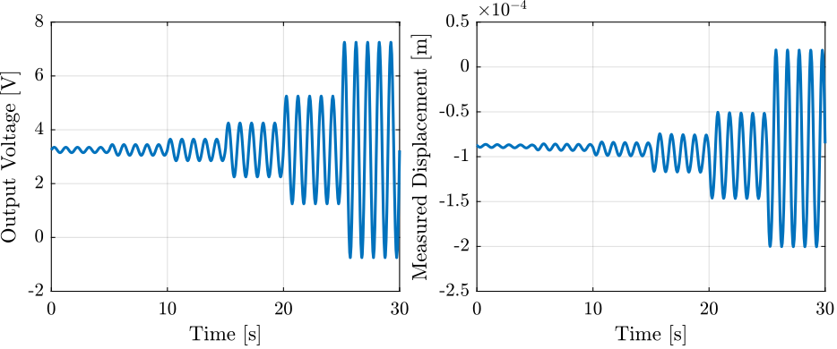
For each amplitude, we only take the last sinus in order to reduce possible transients. Also, it is centered on zero.
The measured displacement at a function of the output voltage are shown in Figure fig:hyst_results_multi_ampl.
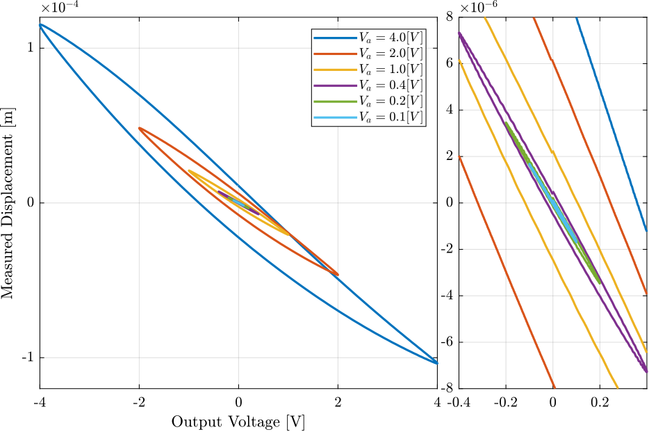
It is quite clear that hysteresis is increasing with the excitation amplitude.
Also, no hysteresis is found on the sensor stack voltage.
FRF Identification - Setup
The identification is performed in three steps:
- White noise excitation with small amplitude. This is used to determine the main resonance of the system.
- Sweep sine excitation with the amplitude lowered around the resonance. The sweep sine is from 10Hz to 400Hz.
- High frequency noise. The noise is band-passed between 300Hz and 2kHz.
Then, the result of the second identification is used between 10Hz and 350Hz and the result of the third identification if used between 350Hz and 2kHz.
Here are the APA numbers that have been measured.
apa_nums = [1 2 4 5 6 7 8];The data are loaded for both the second and third identification:
%% Second identification
apa_sweep = {};
for i = 1:length(apa_nums)
    apa_sweep(i) = {load(sprintf('frf_data_%i_sweep.mat', apa_nums(i)), 't', 'Va', 'Vs', 'de', 'da')};
end

%% Third identification
apa_noise_hf = {};
for i = 1:length(apa_nums)
    apa_noise_hf(i) = {load(sprintf('frf_data_%i_noise_hf.mat', apa_nums(i)), 't', 'Va', 'Vs', 'de', 'da')};
end
The time is the same for all measurements.
%% Time vector
t = apa_sweep{1}.t - apa_sweep{1}.t(1) ; % Time vector [s]

%% Sampling
Ts = (t(end) - t(1))/(length(t)-1); % Sampling Time [s]
Fs = 1/Ts; % Sampling Frequency [Hz]
Then we defined a "Hanning" windows that will be used for the spectral analysis:
win = hanning(ceil(0.5*Fs)); % Hannning WindowsWe get the frequency vector that will be the same for all the frequency domain analysis.
% Only used to have the frequency vector "f"
[~, f] = tfestimate(apa_sweep{1}.Va, apa_sweep{1}.de, win, [], [], 1/Ts);
FRF Identification - DVF
In this section, the dynamics from $V_a$ to $d_e$ is identified.
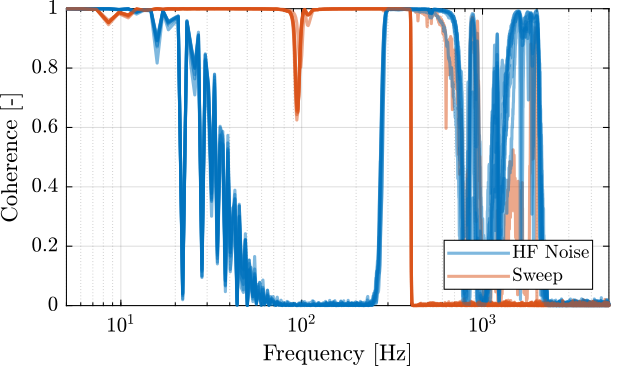
We compute the coherence for 2nd and 3rd identification:
%% Coherence computation
coh_sweep = zeros(length(f), length(apa_nums));
for i = 1:length(apa_nums)
    [coh, ~] = mscohere(apa_sweep{i}.Va, apa_sweep{i}.de, win, [], [], 1/Ts);
    coh_sweep(:, i) = coh;
end

coh_noise_hf = zeros(length(f), length(apa_nums));
for i = 1:length(apa_nums)
    [coh, ~] = mscohere(apa_noise_hf{i}.Va, apa_noise_hf{i}.de, win, [], [], 1/Ts);
    coh_noise_hf(:, i) = coh;
end
The coherence is shown in Figure fig:frf_dvf_plant_coh. It is clear that the Sweep sine gives good coherence up to 400Hz and that the high frequency noise excitation signal helps increasing a little bit the coherence at high frequency.
Then, the transfer function from the DAC output voltage $V_a$ to the measured displacement by the encoders is computed:
%% Transfer function estimation
dvf_sweep = zeros(length(f), length(apa_nums));
for i = 1:length(apa_nums)
    [frf, ~] = tfestimate(apa_sweep{i}.Va, apa_sweep{i}.de, win, [], [], 1/Ts);
    dvf_sweep(:, i) = frf;
end

dvf_noise_hf = zeros(length(f), length(apa_nums));
for i = 1:length(apa_nums)
    [frf, ~] = tfestimate(apa_noise_hf{i}.Va, apa_noise_hf{i}.de, win, [], [], 1/Ts);
    dvf_noise_hf(:, i) = frf;
end
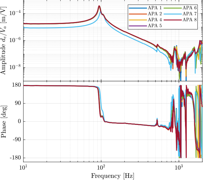
The obtained transfer functions are shown in Figure fig:frf_dvf_plant_tf.
They are all superimposed except for the APA7.
Why is the APA7 off? We could think that the APA7 is stiffer, but also the mass line is off.
It seems that there is a "gain" problem. The encoder seems fine (it measured the same as the Interferometer). Maybe it could be due to the amplifier?
Why is there a double resonance at around 94Hz?
FRF Identification - IFF
In this section, the dynamics from $V_a$ to $V_s$ is identified.
First the coherence is computed and shown in Figure fig:frf_iff_plant_coh. The coherence is very nice from 10Hz to 2kHz. It is only dropping near a zeros at 40Hz, and near the resonance at 95Hz (the excitation amplitude being lowered).
%% Coherence
coh_sweep = zeros(length(f), length(apa_nums));
for i = 1:length(apa_nums)
    [coh, ~] = mscohere(apa_sweep{i}.Va, apa_sweep{i}.Vs, win, [], [], 1/Ts);
    coh_sweep(:, i) = coh;
end

coh_noise_hf = zeros(length(f), length(apa_nums));
for i = 1:length(apa_nums)
    [coh, ~] = mscohere(apa_noise_hf{i}.Va, apa_noise_hf{i}.Vs, win, [], [], 1/Ts);
    coh_noise_hf(:, i) = coh;
end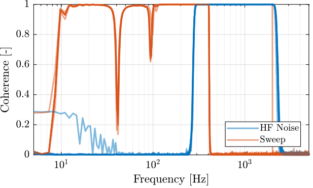
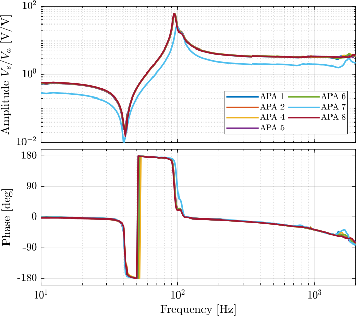
Then the FRF are estimated and shown in Figure fig:frf_iff_plant_tf
%% FRF estimation of the transfer function from Va to Vs
iff_sweep = zeros(length(f), length(apa_nums));
for i = 1:length(apa_nums)
    [frf, ~] = tfestimate(apa_sweep{i}.Va, apa_sweep{i}.Vs, win, [], [], 1/Ts);
    iff_sweep(:, i) = frf;
end

iff_noise_hf = zeros(length(f), length(apa_nums));
for i = 1:length(apa_nums)
    [frf, ~] = tfestimate(apa_noise_hf{i}.Va, apa_noise_hf{i}.Vs, win, [], [], 1/Ts);
    iff_noise_hf(:, i) = frf;
end
#+caption:Identified IFF Plant
Effect of the resistor on the IFF Plant
A resistor is added in parallel with the sensor stack. This has the effect to form a high pass filter with the capacitance of the stack.
We here measured the low frequency transfer function from $V_a$ to $V_s$ with and without this resistor.
% With the resistor
wi_k = load('frf_data_2_sweep_lf_with_R.mat', 't', 'Vs', 'Va');

% Without the resistor
wo_k = load('frf_data_2_sweep_lf.mat',        't', 'Vs', 'Va');
t = wo_k.t; % Time vector [s]
Ts = (t(end) - t(1))/(length(t)-1); % Sampling Time [s]
Fs = 1/Ts; % Sampling Frequency [Hz]We use a very long "Hanning" window for the spectral analysis in order to estimate the low frequency behavior.
win = hanning(ceil(50*Fs)); % Hannning WindowsAnd we estimate the transfer function from $V_a$ to $V_s$ in both cases:
[frf_wo_k, f] = tfestimate(wo_k.Va, wo_k.Vs, win, [], [], 1/Ts);
[frf_wi_k, ~] = tfestimate(wi_k.Va, wi_k.Vs, win, [], [], 1/Ts);
f0 = 0.35;
G_hpf = 0.6*(s/2*pi*f0)/(1 + s/2*pi*f0);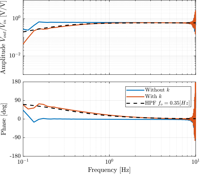
TODO Measurement on Strut 1
Introduction ignore
Measurements are first performed on the strut number 1 with:
- APA 1
- flex 1 and flex 2
Without Encoder
FRF Identification - Setup
The identification is performed in three steps:
- White noise excitation with small amplitude. This is used to determine the main resonance of the system.
- Sweep sine excitation with the amplitude lowered around the resonance. The sweep sine is from 10Hz to 400Hz.
- High frequency noise. The noise is band-passed between 300Hz and 2kHz.
Then, the result of the second identification is used between 10Hz and 350Hz and the result of the third identification if used between 350Hz and 2kHz.
leg_sweep    = load(sprintf('frf_data_leg_%i_sweep.mat',    1), 't', 'Va', 'Vs', 'de', 'da');
leg_noise_hf = load(sprintf('frf_data_leg_%i_noise_hf.mat', 1), 't', 'Va', 'Vs', 'de', 'da');
The time is the same for all measurements.
%% Time vector
t = leg_sweep.t - leg_sweep.t(1) ; % Time vector [s]

%% Sampling
Ts = (t(end) - t(1))/(length(t)-1); % Sampling Time [s]
Fs = 1/Ts; % Sampling Frequency [Hz]
Then we defined a "Hanning" windows that will be used for the spectral analysis:
win = hanning(ceil(0.5*Fs)); % Hannning WindowsWe get the frequency vector that will be the same for all the frequency domain analysis.
% Only used to have the frequency vector "f"
[~, f] = tfestimate(leg_sweep.Va, leg_sweep.de, win, [], [], 1/Ts);
TODO FRF Identification - DVF
In this section, the dynamics from $V_a$ to $d_e$ is identified.
We compute the coherence for 2nd and 3rd identification:
[coh_sweep, ~]    = mscohere(leg_sweep.Va,    leg_sweep.da,    win, [], [], 1/Ts);
[coh_noise_hf, ~] = mscohere(leg_noise_hf.Va, leg_noise_hf.da, win, [], [], 1/Ts);
[dvf_sweep, ~]    = tfestimate(leg_sweep.Va,    leg_sweep.da,    win, [], [], 1/Ts);
[dvf_noise_hf, ~] = tfestimate(leg_noise_hf.Va, leg_noise_hf.da, win, [], [], 1/Ts);
The obtained transfer functions are shown in Figure fig:frf_dvf_plant_tf.
They are all superimposed except for the APA7.
Why is the APA7 off? We could think that the APA7 is stiffer, but also the mass line is off.
It seems that there is a "gain" problem. The encoder seems fine (it measured the same as the Interferometer). Maybe it could be due to the amplifier?
Why is there a double resonance at around 94Hz?

TODO FRF Identification - IFF
In this section, the dynamics from $V_a$ to $V_s$ is identified.
First the coherence is computed and shown in Figure fig:frf_iff_plant_coh. The coherence is very nice from 10Hz to 2kHz. It is only dropping near a zeros at 40Hz, and near the resonance at 95Hz (the excitation amplitude being lowered).
[coh_sweep, ~] = mscohere(leg_sweep.Va, leg_sweep.Vs, win, [], [], 1/Ts);
[coh_noise_hf, ~] = mscohere(leg_noise_hf.Va, leg_noise_hf.Vs, win, [], [], 1/Ts);
Then the FRF are estimated and shown in Figure fig:frf_iff_plant_tf
[iff_sweep, ~] = tfestimate(leg_sweep.Va, leg_sweep.Vs, win, [], [], 1/Ts);
[iff_noise_hf, ~] = tfestimate(leg_noise_hf.Va, leg_noise_hf.Vs, win, [], [], 1/Ts);
#+caption:Identified IFF Plant

With Encoder
FRF Identification - Setup
The identification is performed in three steps:
- White noise excitation with small amplitude. This is used to determine the main resonance of the system.
- Sweep sine excitation with the amplitude lowered around the resonance. The sweep sine is from 10Hz to 400Hz.
- High frequency noise. The noise is band-passed between 300Hz and 2kHz.
Then, the result of the second identification is used between 10Hz and 350Hz and the result of the third identification if used between 350Hz and 2kHz.
leg_enc_sweep    = load(sprintf('frf_data_leg_coder_%i_noise.mat',    1), 't', 'Va', 'Vs', 'de', 'da');
leg_enc_noise_hf = load(sprintf('frf_data_leg_coder_%i_noise_hf.mat', 1), 't', 'Va', 'Vs', 'de', 'da');
TODO FRF Identification - DVF
In this section, the dynamics from $V_a$ to $d_e$ is identified.
We compute the coherence for 2nd and 3rd identification:
[coh_enc_sweep, ~]    = mscohere(leg_enc_sweep.Va,    leg_enc_sweep.de,    win, [], [], 1/Ts);
[coh_enc_noise_hf, ~] = mscohere(leg_enc_noise_hf.Va, leg_enc_noise_hf.de, win, [], [], 1/Ts);
[dvf_enc_sweep, ~]    = tfestimate(leg_enc_sweep.Va,    leg_enc_sweep.de,    win, [], [], 1/Ts);
[dvf_enc_noise_hf, ~] = tfestimate(leg_enc_noise_hf.Va, leg_enc_noise_hf.de, win, [], [], 1/Ts);
The obtained transfer functions are shown in Figure fig:frf_dvf_plant_tf.
They are all superimposed except for the APA7.
Why is the APA7 off? We could think that the APA7 is stiffer, but also the mass line is off.
It seems that there is a "gain" problem. The encoder seems fine (it measured the same as the Interferometer). Maybe it could be due to the amplifier?
Why is there a double resonance at around 94Hz?

Comparison with Interferometer
[dvf_int_sweep, ~]    = tfestimate(leg_enc_sweep.Va,    leg_enc_sweep.da,    win, [], [], 1/Ts);
[dvf_int_noise_hf, ~] = tfestimate(leg_enc_noise_hf.Va, leg_enc_noise_hf.da, win, [], [], 1/Ts);
Clearly using the encoder like this will not be useful.
Probably, the encoders will have to be fixed on the plates so that the resonances of the APA are not a problem anymore.
APA Resonances Frequency
This is very close to what was estimated using the FEM.
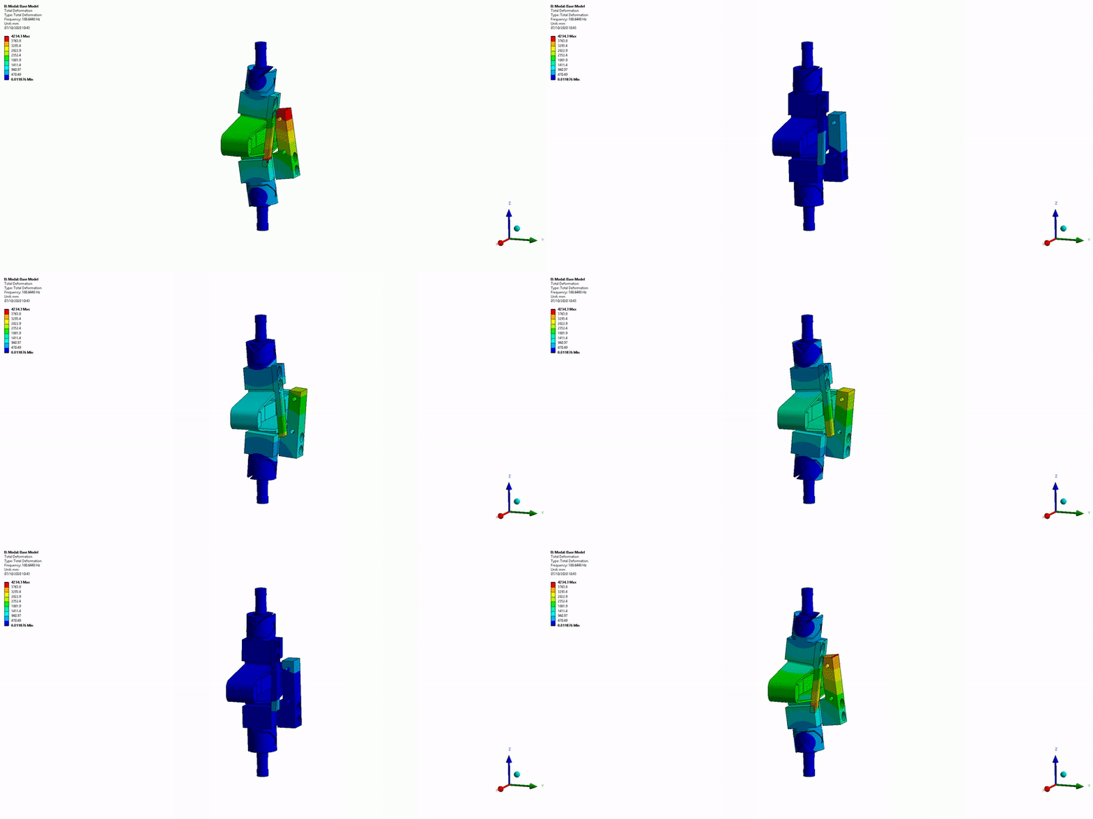
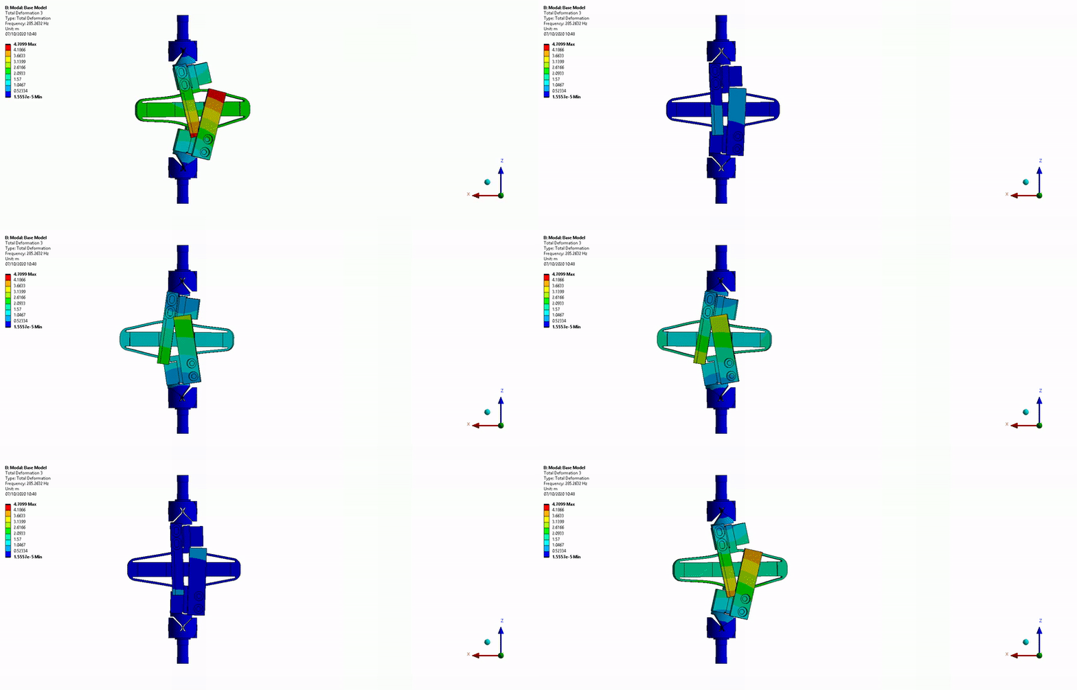
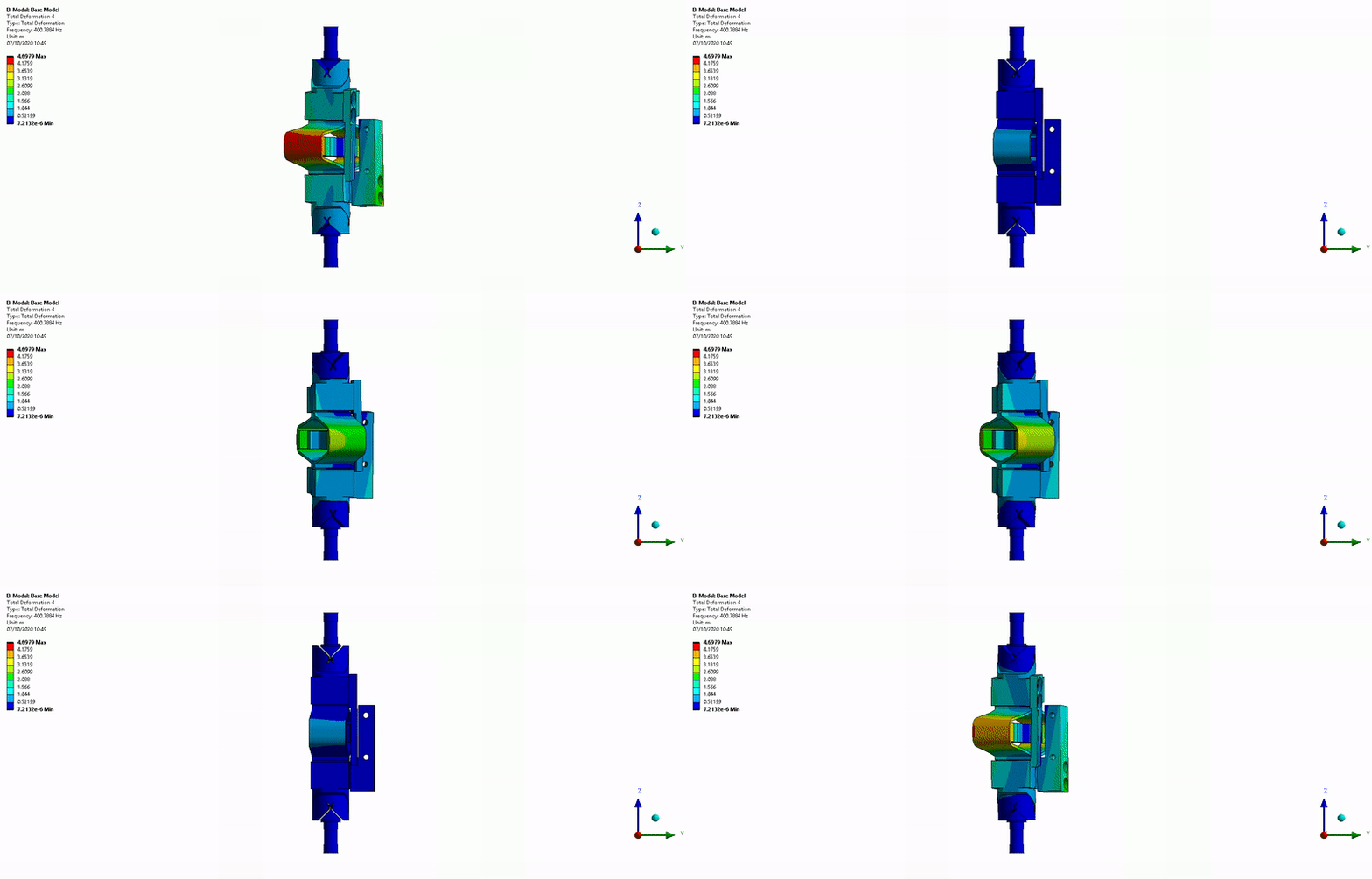
The resonances are indeed due to limited stiffness of the APA.
FRF Identification - IFF
In this section, the dynamics from $V_a$ to $V_s$ is identified.
First the coherence is computed and shown in Figure fig:frf_iff_plant_coh. The coherence is very nice from 10Hz to 2kHz. It is only dropping near a zeros at 40Hz, and near the resonance at 95Hz (the excitation amplitude being lowered).
[coh_enc_sweep,    ~] = mscohere(leg_enc_sweep.Va,    leg_enc_sweep.Vs,    win, [], [], 1/Ts);
[coh_enc_noise_hf, ~] = mscohere(leg_enc_noise_hf.Va, leg_enc_noise_hf.Vs, win, [], [], 1/Ts);
Then the FRF are estimated and shown in Figure fig:frf_iff_plant_tf
[iff_enc_sweep,    ~] = tfestimate(leg_enc_sweep.Va,    leg_enc_sweep.Vs,    win, [], [], 1/Ts);
[iff_enc_noise_hf, ~] = tfestimate(leg_enc_noise_hf.Va, leg_enc_noise_hf.Vs, win, [], [], 1/Ts);
#+caption:Identified IFF Plant

Comparison to when the encoder is not fixed
[iff_sweep, ~]    = tfestimate(leg_sweep.Va,    leg_sweep.Vs,    win, [], [], 1/Ts);
[iff_noise_hf, ~] = tfestimate(leg_noise_hf.Va, leg_noise_hf.Vs, win, [], [], 1/Ts);
We can see that the IFF does not change whether of not the encoder are fixed to the struts.
Measurement Results
Test Bench APA300ML - Simscape Model
Introduction
Nano Hexapod object
n_hexapod = struct();APA - 2 DoF
n_hexapod.actuator = struct();

n_hexapod.actuator.type = 1;

n_hexapod.actuator.k  = ones(6,1)*0.35e6; % [N/m]
n_hexapod.actuator.ke = ones(6,1)*1.5e6; % [N/m]
n_hexapod.actuator.ka = ones(6,1)*43e6; % [N/m]

n_hexapod.actuator.c  = ones(6,1)*3e1; % [N/(m/s)]
n_hexapod.actuator.ce = ones(6,1)*1e1; % [N/(m/s)]
n_hexapod.actuator.ca = ones(6,1)*1e1; % [N/(m/s)]

n_hexapod.actuator.Leq = ones(6,1)*0.056; % [m]

n_hexapod.actuator.Ga = ones(6,1)*1; % Actuator gain [N/V]
n_hexapod.actuator.Gs = ones(6,1)*1; % Sensor gain [V/m]
APA - Flexible Frame
n_hexapod.actuator.type = 2;

n_hexapod.actuator.K = readmatrix('APA300ML_b_mat_K.CSV'); % Stiffness Matrix
n_hexapod.actuator.M = readmatrix('APA300ML_b_mat_M.CSV'); % Mass Matrix
n_hexapod.actuator.xi = 0.01; % Damping ratio
n_hexapod.actuator.P = extractNodes('APA300ML_b_out_nodes_3D.txt'); % Node coordinates [m]

n_hexapod.actuator.ks = 235e6; % Stiffness of one stack [N/m]
n_hexapod.actuator.cs = 1e1; % Stiffness of one stack [N/m]

n_hexapod.actuator.Ga = ones(6,1)*1; % Actuator gain [N/V]
n_hexapod.actuator.Gs = ones(6,1)*1; % Sensor gain [V/m]
APA - Fully Flexible
n_hexapod.actuator.type = 3;

n_hexapod.actuator.K = readmatrix('APA300ML_full_mat_K.CSV'); % Stiffness Matrix
n_hexapod.actuator.M = readmatrix('APA300ML_full_mat_M.CSV'); % Mass Matrix
n_hexapod.actuator.xi = 0.01; % Damping ratio
n_hexapod.actuator.P = extractNodes('APA300ML_full_out_nodes_3D.txt'); % Node coordiantes [m]

n_hexapod.actuator.Ga = ones(6,1)*1; % Actuator gain [N/V]
n_hexapod.actuator.Gs = ones(6,1)*1; % Sensor gain [V/m]
Identification
%% Options for Linearized
options = linearizeOptions;
options.SampleTime = 0;

%% Name of the Simulink File
mdl = 'test_bench_apa300ml';

%% Input/Output definition
clear io; io_i = 1;
io(io_i) = linio([mdl, '/Va'],  1, 'openinput');  io_i = io_i + 1; % Actuator Voltage
io(io_i) = linio([mdl, '/Vs'],  1, 'openoutput'); io_i = io_i + 1; % Sensor Voltage
io(io_i) = linio([mdl, '/dL'],  1, 'openoutput'); io_i = io_i + 1; % Relative Motion Outputs
io(io_i) = linio([mdl, '/z'],   1, 'openoutput'); io_i = io_i + 1; % Vertical Motion

%% Run the linearization
Ga = linearize(mdl, io, 0.0, options);
Ga.InputName  = {'Va'};
Ga.OutputName = {'Vs', 'dL', 'z'};
Compare 2-DoF with flexible
APA - 2 DoF
n_hexapod = struct();

n_hexapod.actuator = struct();

n_hexapod.actuator.type = 1;

n_hexapod.actuator.k  = ones(6,1)*0.35e6; % [N/m]
n_hexapod.actuator.ke = ones(6,1)*1.5e6; % [N/m]
n_hexapod.actuator.ka = ones(6,1)*43e6; % [N/m]

n_hexapod.actuator.c  = ones(6,1)*3e1; % [N/(m/s)]
n_hexapod.actuator.ce = ones(6,1)*1e1; % [N/(m/s)]
n_hexapod.actuator.ca = ones(6,1)*1e1; % [N/(m/s)]

n_hexapod.actuator.Leq = ones(6,1)*0.056; % [m]

n_hexapod.actuator.Ga = ones(6,1)*-2.15; % Actuator gain [N/V]
n_hexapod.actuator.Gs = ones(6,1)*2.305e-08; % Sensor gain [V/m]
G_2dof = linearize(mdl, io, 0.0, options);
G_2dof.InputName = {'Va'};
G_2dof.OutputName = {'Vs', 'dL', 'z'};APA - Fully Flexible
n_hexapod = struct();

n_hexapod.actuator.type = 3;

n_hexapod.actuator.K = readmatrix('APA300ML_full_mat_K.CSV'); % Stiffness Matrix
n_hexapod.actuator.M = readmatrix('APA300ML_full_mat_M.CSV'); % Mass Matrix
n_hexapod.actuator.xi = 0.01; % Damping ratio
n_hexapod.actuator.P = extractNodes('APA300ML_full_out_nodes_3D.txt'); % Node coordiantes [m]

n_hexapod.actuator.Ga = ones(6,1)*1; % Actuator gain [N/V]
n_hexapod.actuator.Gs = ones(6,1)*1; % Sensor gain [V/m]
G_flex = linearize(mdl, io, 0.0, options);
G_flex.InputName = {'Va'};
G_flex.OutputName = {'Vs', 'dL', 'z'};Comparison
Test Bench Struts - Simscape Model
Introduction
Nano Hexapod object
n_hexapod = struct();Flexible Joint - Bot
n_hexapod.flex_bot = struct();

n_hexapod.flex_bot.type = 1; % 1: 2dof / 2: 3dof / 3: 4dof

n_hexapod.flex_bot.kRx = ones(6,1)*5; % X bending stiffness [Nm/rad]
n_hexapod.flex_bot.kRy = ones(6,1)*5; % Y bending stiffness [Nm/rad]
n_hexapod.flex_bot.kRz = ones(6,1)*260; % Torsionnal stiffness [Nm/rad]
n_hexapod.flex_bot.kz  = ones(6,1)*1e8; % Axial stiffness [N/m]

n_hexapod.flex_bot.cRx = ones(6,1)*0.1; % [Nm/(rad/s)]
n_hexapod.flex_bot.cRy = ones(6,1)*0.1; % [Nm/(rad/s)]
n_hexapod.flex_bot.cRz = ones(6,1)*0.1; % [Nm/(rad/s)]
n_hexapod.flex_bot.cz  = ones(6,1)*1e2; %[N/(m/s)]
Flexible Joint - Top
n_hexapod.flex_top = struct();

n_hexapod.flex_top.type = 2; % 1: 2dof / 2: 3dof / 3: 4dof

n_hexapod.flex_top.kRx = ones(6,1)*5; % X bending stiffness [Nm/rad]
n_hexapod.flex_top.kRy = ones(6,1)*5; % Y bending stiffness [Nm/rad]
n_hexapod.flex_top.kRz = ones(6,1)*260; % Torsionnal stiffness [Nm/rad]
n_hexapod.flex_top.kz  = ones(6,1)*1e8; % Axial stiffness [N/m]

n_hexapod.flex_top.cRx = ones(6,1)*0.1; % [Nm/(rad/s)]
n_hexapod.flex_top.cRy = ones(6,1)*0.1; % [Nm/(rad/s)]
n_hexapod.flex_top.cRz = ones(6,1)*0.1; % [Nm/(rad/s)]
n_hexapod.flex_top.cz  = ones(6,1)*1e2; %[N/(m/s)]
APA - 2 DoF
n_hexapod.actuator = struct();

n_hexapod.actuator.type = 1;

n_hexapod.actuator.k  = ones(6,1)*0.35e6; % [N/m]
n_hexapod.actuator.ke = ones(6,1)*1.5e6; % [N/m]
n_hexapod.actuator.ka = ones(6,1)*43e6; % [N/m]

n_hexapod.actuator.c  = ones(6,1)*3e1; % [N/(m/s)]
n_hexapod.actuator.ce = ones(6,1)*1e1; % [N/(m/s)]
n_hexapod.actuator.ca = ones(6,1)*1e1; % [N/(m/s)]

n_hexapod.actuator.Leq = ones(6,1)*0.056; % [m]

n_hexapod.actuator.Ga = ones(6,1)*1; % Actuator gain [N/V]
n_hexapod.actuator.Gs = ones(6,1)*1; % Sensor gain [V/m]
APA - Flexible Frame
n_hexapod.actuator.type = 2;

n_hexapod.actuator.K = readmatrix('APA300ML_b_mat_K.CSV'); % Stiffness Matrix
n_hexapod.actuator.M = readmatrix('APA300ML_b_mat_M.CSV'); % Mass Matrix
n_hexapod.actuator.xi = 0.01; % Damping ratio
n_hexapod.actuator.P = extractNodes('APA300ML_b_out_nodes_3D.txt'); % Node coordinates [m]

n_hexapod.actuator.ks = 235e6; % Stiffness of one stack [N/m]
n_hexapod.actuator.cs = 1e1; % Stiffness of one stack [N/m]

n_hexapod.actuator.Ga = ones(6,1)*1; % Actuator gain [N/V]
n_hexapod.actuator.Gs = ones(6,1)*1; % Sensor gain [V/m]
APA - Fully Flexible
n_hexapod.actuator.type = 3;

n_hexapod.actuator.K = readmatrix('APA300ML_full_mat_K.CSV'); % Stiffness Matrix
n_hexapod.actuator.M = readmatrix('APA300ML_full_mat_M.CSV'); % Mass Matrix
n_hexapod.actuator.xi = 0.01; % Damping ratio
n_hexapod.actuator.P = extractNodes('APA300ML_full_out_nodes_3D.txt'); % Node coordiantes [m]

n_hexapod.actuator.Ga = ones(6,1)*1; % Actuator gain [N/V]
n_hexapod.actuator.Gs = ones(6,1)*1; % Sensor gain [V/m]
Identification
%% Options for Linearized
options = linearizeOptions;
options.SampleTime = 0;

%% Name of the Simulink File
mdl = 'test_bench_struts';

%% Input/Output definition
clear io; io_i = 1;
io(io_i) = linio([mdl, '/Va'],  1, 'openinput');  io_i = io_i + 1; % Actuator Voltage
io(io_i) = linio([mdl, '/Vs'],  1, 'openoutput'); io_i = io_i + 1; % Sensor Voltage
io(io_i) = linio([mdl, '/dL'],  1, 'openoutput'); io_i = io_i + 1; % Relative Motion Outputs
io(io_i) = linio([mdl, '/z'],   1, 'openoutput'); io_i = io_i + 1; % Vertical Motion

%% Run the linearization
Gs = linearize(mdl, io, 0.0, options);
Gs.InputName  = {'Va'};
Gs.OutputName = {'Vs', 'dL', 'z'};
Compare flexible joints
Perfect
n_hexapod.flex_bot.type = 1; % 1: 2dof / 2: 3dof / 3: 4dof
n_hexapod.flex_top.type = 2; % 1: 2dof / 2: 3dof / 3: 4dof
Gp = linearize(mdl, io, 0.0, options);
Gp.InputName = {'Va'};
Gp.OutputName = {'Vs', 'dL', 'z'};Top Flexible
n_hexapod.flex_bot.type = 1; % 1: 2dof / 2: 3dof / 3: 4dof
n_hexapod.flex_top.type = 3; % 1: 2dof / 2: 3dof / 3: 4dof
Gt = linearize(mdl, io, 0.0, options);
Gt.InputName = {'Va'};
Gt.OutputName = {'Vs', 'dL', 'z'};Bottom Flexible
n_hexapod.flex_bot.type = 3; % 1: 2dof / 2: 3dof / 3: 4dof
n_hexapod.flex_top.type = 2; % 1: 2dof / 2: 3dof / 3: 4dof
Gb = linearize(mdl, io, 0.0, options);
Gb.InputName = {'Va'};
Gb.OutputName = {'Vs', 'dL', 'z'};Both Flexible
n_hexapod.flex_bot.type = 3; % 1: 2dof / 2: 3dof / 3: 4dof
n_hexapod.flex_top.type = 3; % 1: 2dof / 2: 3dof / 3: 4dof
Gf = linearize(mdl, io, 0.0, options);
Gf.InputName = {'Va'};
Gf.OutputName = {'Vs', 'dL', 'z'};Comparison
Resonance frequencies - APA300ML
Introduction
Three main resonances are foreseen to be problematic for the control of the APA300ML:
- Mode in X-bending at 189Hz (Figure fig:mode_bending_x)
- Mode in Y-bending at 285Hz (Figure fig:mode_bending_y)
- Mode in Z-torsion at 400Hz (Figure fig:mode_torsion_z)


These modes are present when flexible joints are fixed to the ends of the APA300ML.
In this section, we try to find the resonance frequency of these modes when one end of the APA is fixed and the other is free.
Setup
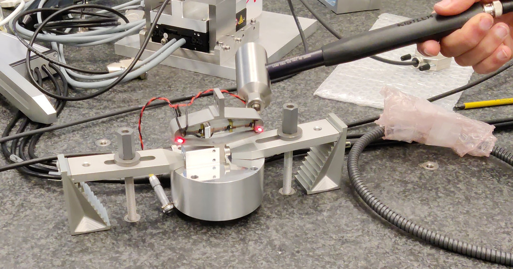
The measurement setup is shown in Figure fig:measurement_setup_torsion. A Laser vibrometer is measuring the difference of motion of two points. The APA is excited with an instrumented hammer and the transfer function from the hammer to the measured rotation is computed.
- Laser Doppler Vibrometer Polytec OFV512
- Instrumented hammer
Bending - X
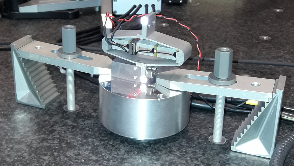
The setup to measure the X-bending motion is shown in Figure fig:measurement_setup_X_bending. The APA is excited with an instrumented hammer having a solid metallic tip. The impact point is on the back-side of the APA aligned with the top measurement point.
The data is loaded.
bending_X = load('apa300ml_bending_X_top.mat');
The config for tfestimate is performed:
Ts = bending_X.Track1_X_Resolution; % Sampling frequency [Hz]
win = hann(ceil(1/Ts));
The transfer function from the input force to the output "rotation" (difference between the two measured distances).
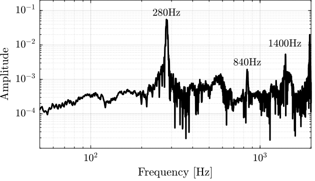
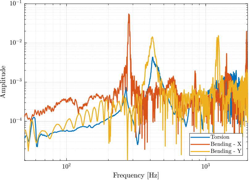
[G_bending_X, f] = tfestimate(bending_X.Track1, bending_X.Track2, win, [], [], 1/Ts);The result is shown in Figure fig:apa300ml_meas_freq_bending_x.
The can clearly observe a nice peak at 280Hz, and then peaks at the odd "harmonics" (third "harmonic" at 840Hz, and fifth "harmonic" at 1400Hz).
Bending - Y
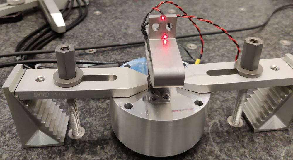
The setup to measure the Y-bending is shown in Figure fig:measurement_setup_Y_bending.
The impact point of the instrumented hammer is located on the back surface of the top interface (on the back of the 2 measurements points).
The data is loaded, and the transfer function from the force to the measured rotation is computed.
bending_Y = load('apa300ml_bending_Y_top.mat');
[G_bending_Y, ~]  = tfestimate(bending_Y.Track1, bending_Y.Track2, win, [], [], 1/Ts);
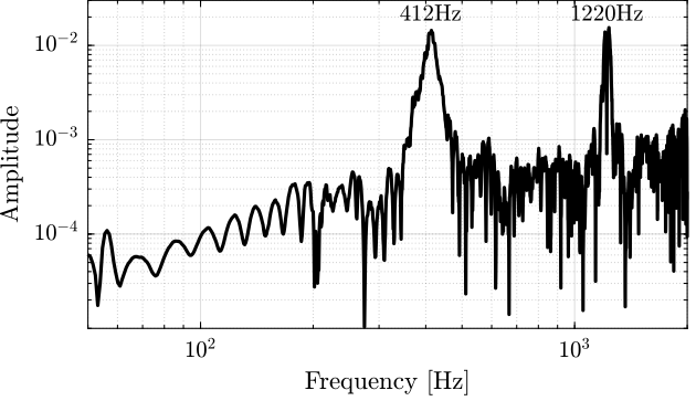
The results are shown in Figure fig:apa300ml_meas_freq_bending_y. The main resonance is at 412Hz, and we also see the third "harmonic" at 1220Hz.
Torsion - Z
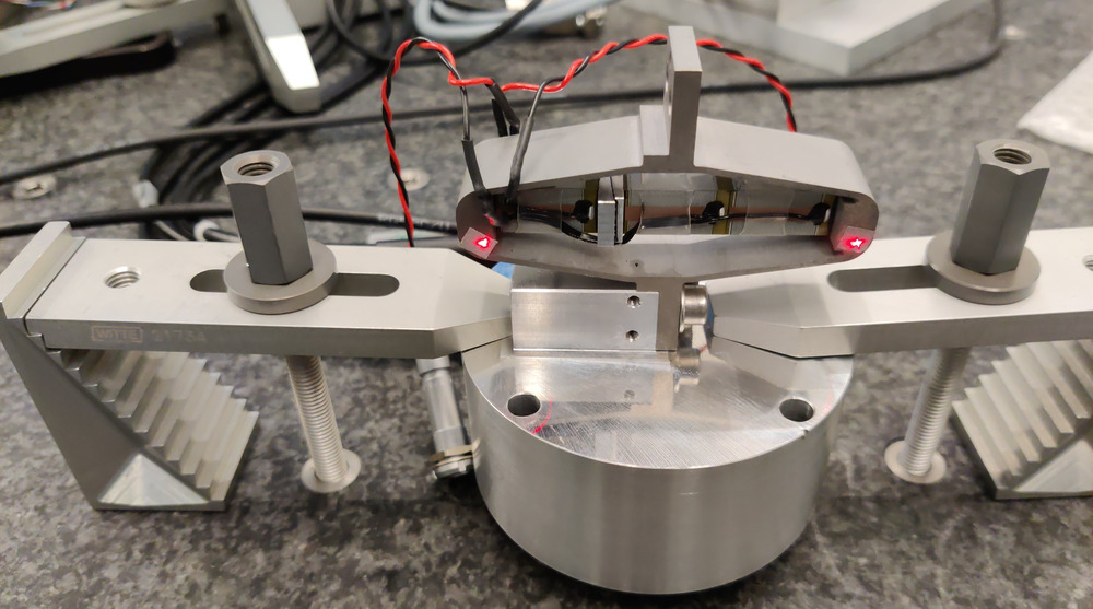
Finally, we measure the Z-torsion resonance as shown in Figure fig:measurement_setup_torsion_bis.
The excitation is shown on the other side of the APA, on the side to excite the torsion motion.
The data is loaded, and the transfer function computed.
torsion = load('apa300ml_torsion_left.mat');
[G_torsion, ~]  = tfestimate(torsion.Track1, torsion.Track2, win, [], [], 1/Ts);
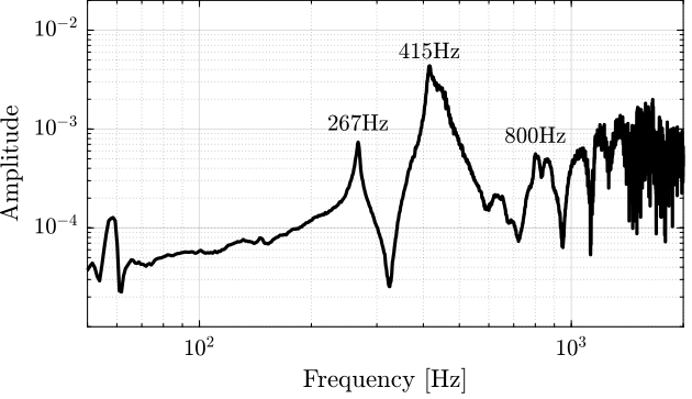
The results are shown in Figure fig:apa300ml_meas_freq_torsion_z. We observe a first peak at 267Hz, which corresponds to the X-bending mode that was measured at 280Hz. And then a second peak at 415Hz, which corresponds to the X-bending mode that was measured at 412Hz. The mode in pure torsion is probably at higher frequency (peak around 1kHz?).
In order to verify that, the APA is excited on the top part such that the torsion mode should not be excited.
torsion = load('apa300ml_torsion_top.mat');
[G_torsion_top, ~]  = tfestimate(torsion.Track1, torsion.Track2, win, [], [], 1/Ts);
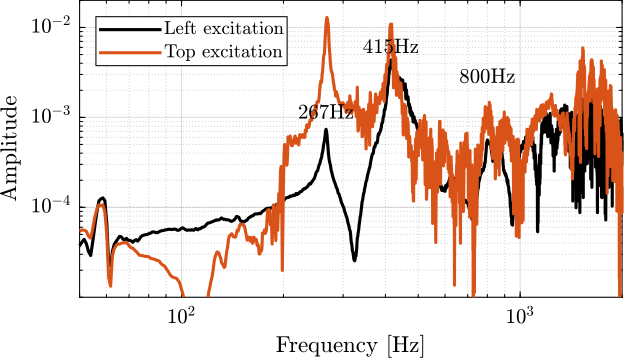
The two FRF are compared in Figure fig:apa300ml_meas_freq_torsion_z_comp. It is clear that the first two modes does not correspond to the torsional mode. Maybe the resonance at 800Hz, or even higher resonances. It is difficult to conclude here.
Compare
The three measurements are shown in Figure fig:apa300ml_meas_freq_compare.
Conclusion
When two flexible joints are fixed at each ends of the APA, the APA is mostly in a free/free condition in terms of bending/torsion (the bending/torsional stiffness of the joints being very small).
In the current tests, the APA are in a fixed/free condition. Therefore, it is quite obvious that we measured higher resonance frequencies than what is foreseen for the struts. It is however quite interesting that there is a factor $\approx \sqrt{2}$ between the two (increased of the stiffness by a factor 2?).
| Mode | Strut Mode | Measured Frequency |
|---|---|---|
| X-Bending | 189Hz | 280Hz |
| Y-Bending | 285Hz | 410Hz |
| Z-Torsion | 400Hz | ? |
Function
generateSweepExc: Generate sweep sinus excitation
<<sec:generateSweepExc>>
Function description
function [U_exc] = generateSweepExc(args)
% generateSweepExc - Generate a Sweep Sine excitation signal
%
% Syntax: [U_exc] = generateSweepExc(args)
%
% Inputs:
%    - args - Optinal arguments:
%        - Ts              - Sampling Time                                              - [s]
%        - f_start         - Start frequency of the sweep                               - [Hz]
%        - f_end           - End frequency of the sweep                                 - [Hz]
%        - V_mean          - Mean value of the excitation voltage                       - [V]
%        - V_exc           - Excitation Amplitude for the Sweep, could be numeric or TF - [V]
%        - t_start         - Time at which the sweep begins                             - [s]
%        - exc_duration    - Duration of the sweep                                      - [s]
%        - sweep_type      - 'logarithmic' or 'linear'                                  - [-]
%        - smooth_ends     - 'true' or 'false': smooth transition between 0 and V_mean  - [-]
Optional Parameters
arguments
    args.Ts              (1,1) double  {mustBeNumeric, mustBePositive} = 1e-4
    args.f_start         (1,1) double  {mustBeNumeric, mustBePositive} = 1
    args.f_end           (1,1) double  {mustBeNumeric, mustBePositive} = 1e3
    args.V_mean          (1,1) double  {mustBeNumeric} = 0
    args.V_exc                                         = 1
    args.t_start         (1,1) double  {mustBeNumeric, mustBeNonnegative} = 5
    args.exc_duration    (1,1) double  {mustBeNumeric, mustBePositive} = 10
    args.sweep_type            char    {mustBeMember(args.sweep_type,{'log', 'lin'})} = 'lin'
    args.smooth_ends           logical {mustBeNumericOrLogical} = true
end
Sweep Sine part
t_sweep = 0:args.Ts:args.exc_duration;

if strcmp(args.sweep_type, 'log')
    V_exc = sin(2*pi*args.f_start * args.exc_duration/log(args.f_end/args.f_start) * (exp(log(args.f_end/args.f_start)*t_sweep/args.exc_duration) - 1));
elseif strcmp(args.sweep_type, 'lin')
    V_exc = sin(2*pi*(args.f_start + (args.f_end - args.f_start)/2/args.exc_duration*t_sweep).*t_sweep);
else
    error('sweep_type should either be equal to "log" or to "lin"');
end
if isnumeric(args.V_exc)
V_sweep = args.V_mean + args.V_exc*V_exc;
elseif isct(args.V_exc)
if strcmp(args.sweep_type, 'log')
V_sweep = args.V_mean + abs(squeeze(freqresp(args.V_exc, args.f_start*(args.f_end/args.f_start).^(t_sweep/args.exc_duration), 'Hz')))'.*V_exc;
elseif strcmp(args.sweep_type, 'lin')
V_sweep = args.V_mean + abs(squeeze(freqresp(args.V_exc, args.f_start+(args.f_end-args.f_start)/args.exc_duration*t_sweep, 'Hz')))'.*V_exc;
end
endSmooth Ends
if args.t_start > 0
    t_smooth_start = args.Ts:args.Ts:args.t_start;

    V_smooth_start = zeros(size(t_smooth_start));
    V_smooth_end   = zeros(size(t_smooth_start));

    if args.smooth_ends
        Vd_max = args.V_mean/(0.7*args.t_start);

        V_d = zeros(size(t_smooth_start));
        V_d(t_smooth_start < 0.2*args.t_start) = t_smooth_start(t_smooth_start < 0.2*args.t_start)*Vd_max/(0.2*args.t_start);
        V_d(t_smooth_start > 0.2*args.t_start & t_smooth_start < 0.7*args.t_start) = Vd_max;
        V_d(t_smooth_start > 0.7*args.t_start & t_smooth_start < 0.9*args.t_start) = Vd_max - (t_smooth_start(t_smooth_start > 0.7*args.t_start & t_smooth_start < 0.9*args.t_start) - 0.7*args.t_start)*Vd_max/(0.2*args.t_start);

        V_smooth_start = cumtrapz(V_d)*args.Ts;

        V_smooth_end = args.V_mean - V_smooth_start;
    end
else
    V_smooth_start = [];
    V_smooth_end = [];
end
Combine Excitation signals
V_exc = [V_smooth_start, V_sweep, V_smooth_end];
t_exc = args.Ts*[0:1:length(V_exc)-1];
U_exc = [t_exc; V_exc];
generateShapedNoise: Generate Shaped Noise excitation
<<sec:generateShapedNoise>>
Function description
function [U_exc] = generateShapedNoise(args)
% generateShapedNoise - Generate a Shaped Noise excitation signal
%
% Syntax: [U_exc] = generateShapedNoise(args)
%
% Inputs:
%    - args - Optinal arguments:
%        - Ts              - Sampling Time                                              - [s]
%        - V_mean          - Mean value of the excitation voltage                       - [V]
%        - V_exc           - Excitation Amplitude, could be numeric or TF               - [V rms]
%        - t_start         - Time at which the noise begins                             - [s]
%        - exc_duration    - Duration of the noise                                      - [s]
%        - smooth_ends     - 'true' or 'false': smooth transition between 0 and V_mean  - [-]
Optional Parameters
arguments
    args.Ts              (1,1) double  {mustBeNumeric, mustBePositive} = 1e-4
    args.V_mean          (1,1) double  {mustBeNumeric} = 0
    args.V_exc                                         = 1
    args.t_start         (1,1) double  {mustBeNumeric, mustBePositive} = 5
    args.exc_duration    (1,1) double  {mustBeNumeric, mustBePositive} = 10
    args.smooth_ends           logical {mustBeNumericOrLogical} = true
end
Shaped Noise
t_noise = 0:args.Ts:args.exc_duration;if isnumeric(args.V_exc)
V_noise = args.V_mean + args.V_exc*sqrt(1/args.Ts/2)*randn(length(t_noise), 1)';
elseif isct(args.V_exc)
V_noise = args.V_mean + lsim(args.V_exc, sqrt(1/args.Ts/2)*randn(length(t_noise), 1), t_noise)';
endSmooth Ends
t_smooth_start = args.Ts:args.Ts:args.t_start;

V_smooth_start = zeros(size(t_smooth_start));
V_smooth_end   = zeros(size(t_smooth_start));

if args.smooth_ends
    Vd_max = args.V_mean/(0.7*args.t_start);

    V_d = zeros(size(t_smooth_start));
    V_d(t_smooth_start < 0.2*args.t_start) = t_smooth_start(t_smooth_start < 0.2*args.t_start)*Vd_max/(0.2*args.t_start);
    V_d(t_smooth_start > 0.2*args.t_start & t_smooth_start < 0.7*args.t_start) = Vd_max;
    V_d(t_smooth_start > 0.7*args.t_start & t_smooth_start < 0.9*args.t_start) = Vd_max - (t_smooth_start(t_smooth_start > 0.7*args.t_start & t_smooth_start < 0.9*args.t_start) - 0.7*args.t_start)*Vd_max/(0.2*args.t_start);

    V_smooth_start = cumtrapz(V_d)*args.Ts;

    V_smooth_end = args.V_mean - V_smooth_start;
end
Combine Excitation signals
V_exc = [V_smooth_start, V_noise, V_smooth_end];
t_exc = args.Ts*[0:1:length(V_exc)-1];
U_exc = [t_exc; V_exc];
generateSinIncreasingAmpl: Generate Sinus with increasing amplitude
<<sec:generateSinIncreasingAmpl>>
Function description
function [U_exc] = generateSinIncreasingAmpl(args)
% generateSinIncreasingAmpl - Generate Sinus with increasing amplitude
%
% Syntax: [U_exc] = generateSinIncreasingAmpl(args)
%
% Inputs:
%    - args - Optinal arguments:
%        - Ts              - Sampling Time                                              - [s]
%        - V_mean          - Mean value of the excitation voltage                       - [V]
%        - sin_ampls       - Excitation Amplitudes                                      - [V]
%        - sin_freq        - Excitation Frequency                                       - [Hz]
%        - sin_num         - Number of period for each amplitude                        - [-]
%        - t_start         - Time at which the excitation begins                        - [s]
%        - smooth_ends     - 'true' or 'false': smooth transition between 0 and V_mean  - [-]
Optional Parameters
arguments
    args.Ts              (1,1) double  {mustBeNumeric, mustBePositive} = 1e-4
    args.V_mean          (1,1) double  {mustBeNumeric} = 0
    args.sin_ampls             double  {mustBeNumeric, mustBePositive} = [0.1, 0.2, 0.3]
    args.sin_period      (1,1) double  {mustBeNumeric, mustBePositive} = 1
    args.sin_num         (1,1) double  {mustBeNumeric, mustBePositive, mustBeInteger} = 3
    args.t_start         (1,1) double  {mustBeNumeric, mustBePositive} = 5
    args.smooth_ends           logical {mustBeNumericOrLogical} = true
end
Sinus excitation
t_noise = 0:args.Ts:args.sin_period*args.sin_num;
sin_exc = [];
for sin_ampl = args.sin_ampls
sin_exc = [sin_exc, args.V_mean + sin_ampl*sin(2*pi/args.sin_period*t_noise)];
endSmooth Ends
t_smooth_start = args.Ts:args.Ts:args.t_start;

V_smooth_start = zeros(size(t_smooth_start));
V_smooth_end   = zeros(size(t_smooth_start));

if args.smooth_ends
    Vd_max = args.V_mean/(0.7*args.t_start);

    V_d = zeros(size(t_smooth_start));
    V_d(t_smooth_start < 0.2*args.t_start) = t_smooth_start(t_smooth_start < 0.2*args.t_start)*Vd_max/(0.2*args.t_start);
    V_d(t_smooth_start > 0.2*args.t_start & t_smooth_start < 0.7*args.t_start) = Vd_max;
    V_d(t_smooth_start > 0.7*args.t_start & t_smooth_start < 0.9*args.t_start) = Vd_max - (t_smooth_start(t_smooth_start > 0.7*args.t_start & t_smooth_start < 0.9*args.t_start) - 0.7*args.t_start)*Vd_max/(0.2*args.t_start);

    V_smooth_start = cumtrapz(V_d)*args.Ts;

    V_smooth_end = args.V_mean - V_smooth_start;
end
Combine Excitation signals
V_exc = [V_smooth_start, sin_exc, V_smooth_end];
t_exc = args.Ts*[0:1:length(V_exc)-1];
U_exc = [t_exc; V_exc];