svd-control/index.org

SVD Control

• Gravimeter - Simscape Model
  • Introduction
  • Simscape Model - Parameters
  • System Identification - Without Gravity
  • System Identification - With Gravity
  • Analytical Model
    • Parameters
    • Generation of the State Space Model
    • Comparison with the Simscape Model
    • Analysis
    • Control Section
    • Greshgorin radius
    • Injecting ground motion in the system to have the output
• Gravimeter - Functions
  • align
  • pzmap_testCL
• Stewart Platform - Simscape Model
  • Introduction
  • Simscape Model - Parameters
  • Identification of the plant
  • Obtained Dynamics
  • Real Approximation of $G$ at the decoupling frequency
  • Verification of the decoupling using the "Gershgorin Radii"
  • Decoupled Plant
  • Diagonal Controller
  • Closed-Loop system Performances

Gravimeter - Simscape Model

Introduction

Model of the gravimeter

Simscape Model - Parameters

  open('gravimeter.slx')

Parameters

  l  = 1.0; % Length of the mass [m]
  la = 0.5; % Position of Act. [m]

  h  = 3.4; % Height of the mass [m]
  ha = 1.7; % Position of Act. [m]

  m = 400; % Mass [kg]
  I = 115; % Inertia [kg m^2]

  k = 15e3; % Actuator Stiffness [N/m]
  c = 0.03; % Actuator Damping [N/(m/s)]

  deq = 0.2; % Length of the actuators [m]

  g = 0; % Gravity [m/s2]

System Identification - Without Gravity

  %% Name of the Simulink File
  mdl = 'gravimeter';

  %% Input/Output definition
  clear io; io_i = 1;
  io(io_i) = linio([mdl, '/F1'], 1, 'openinput');  io_i = io_i + 1;
  io(io_i) = linio([mdl, '/F2'], 1, 'openinput');  io_i = io_i + 1;
  io(io_i) = linio([mdl, '/F3'], 1, 'openinput');  io_i = io_i + 1;
  io(io_i) = linio([mdl, '/Acc_side'], 1, 'openoutput'); io_i = io_i + 1;
  io(io_i) = linio([mdl, '/Acc_side'], 2, 'openoutput'); io_i = io_i + 1;
  io(io_i) = linio([mdl, '/Acc_top'], 1, 'openoutput'); io_i = io_i + 1;
  io(io_i) = linio([mdl, '/Acc_top'], 2, 'openoutput'); io_i = io_i + 1;

  G = linearize(mdl, io);
  G.InputName  = {'F1', 'F2', 'F3'};
  G.OutputName = {'Ax1', 'Az1', 'Ax2', 'Az2'};

pole(G)
ans =
      -0.000473481142385795 +      21.7596190728632i
      -0.000473481142385795 -      21.7596190728632i
      -7.49842879459172e-05 +       8.6593576906982i
      -7.49842879459172e-05 -       8.6593576906982i
       -5.1538686792578e-06 +      2.27025295182756i
       -5.1538686792578e-06 -      2.27025295182756i

The plant as 6 states as expected (2 translations + 1 rotation)

  size(G)

State-space model with 4 outputs, 3 inputs, and 6 states.

Open Loop Transfer Function from 3 Actuators to 4 Accelerometers

System Identification - With Gravity

  g = 9.80665; % Gravity [m/s2]

  Gg = linearize(mdl, io);
  Gg.InputName  = {'F1', 'F2', 'F3'};
  Gg.OutputName = {'Ax1', 'Az1', 'Ax2', 'Az2'};

We can now see that the system is unstable due to gravity.

pole(Gg)
ans =
          -10.9848275341252 +                     0i
           10.9838836405201 +                     0i
      -7.49855379478109e-05 +      8.65962885770051i
      -7.49855379478109e-05 -      8.65962885770051i
      -6.68819548733559e-06 +     0.832960422243848i
      -6.68819548733559e-06 -     0.832960422243848i

Open Loop Transfer Function from 3 Actuators to 4 Accelerometers with an without gravity

Analytical Model

Parameters

Bode options.

  P = bodeoptions;
  P.FreqUnits = 'Hz';
  P.MagUnits = 'abs';
  P.MagScale = 'log';
  P.Grid = 'on';
  P.PhaseWrapping = 'on';
  P.Title.FontSize = 14;
  P.XLabel.FontSize = 14;
  P.YLabel.FontSize = 14;
  P.TickLabel.FontSize = 12;
  P.Xlim = [1e-1,1e2];
  P.MagLowerLimMode = 'manual';
  P.MagLowerLim= 1e-3;

Frequency vector.

  w = 2*pi*logspace(-1,2,1000); % [rad/s]

Generation of the State Space Model

Mass matrix

  M = [m 0 0
       0 m 0
       0 0 I];

Jacobian of the bottom sensor

  Js1 = [1 0  h/2
         0 1 -l/2];

Jacobian of the top sensor

  Js2 = [1 0 -h/2
         0 1  0];

Jacobian of the actuators

  Ja = [1 0  ha   % Left horizontal actuator
        0 1 -la   % Left vertical actuator
        0 1  la]; % Right vertical actuator
  Jta = Ja';

Stiffness and Damping matrices

  K = k*Jta*Ja;
  C = c*Jta*Ja;

State Space Matrices

  E = [1 0 0
       0 1 0
       0 0 1]; %projecting ground motion in the directions of the legs

  AA = [zeros(3) eye(3)
        -M\K -M\C];

  BB = [zeros(3,6)
        M\Jta M\(k*Jta*E)];

  CC = [[Js1;Js2] zeros(4,3);
        zeros(2,6)
        (Js1+Js2)./2 zeros(2,3)
        (Js1-Js2)./2 zeros(2,3)
        (Js1-Js2)./(2*h) zeros(2,3)];

  DD = [zeros(4,6)
        zeros(2,3) eye(2,3)
        zeros(6,6)];

State Space model:

• Input = three actuators and three ground motions
• Output = the bottom sensor; the top sensor; the ground motion; the half sum; the half difference; the rotation

  system_dec = ss(AA,BB,CC,DD);

  size(system_dec)

State-space model with 12 outputs, 6 inputs, and 6 states.

Comparison with the Simscape Model

Comparison of the analytical and the Simscape models

Analysis

  % figure
  % bode(system_dec,P);
  % return

  %% svd decomposition
  % system_dec_freq = freqresp(system_dec,w);
  % S = zeros(3,length(w));
  % for m = 1:length(w)
  %     S(:,m) = svd(system_dec_freq(1:4,1:3,m));
  % end
  % figure
  % loglog(w./(2*pi), S);hold on;
  % % loglog(w./(2*pi), abs(Val(1,:)),w./(2*pi), abs(Val(2,:)),w./(2*pi), abs(Val(3,:)));
  % xlabel('Frequency [Hz]');ylabel('Singular Value [-]');
  % legend('\sigma_1','\sigma_2','\sigma_3');%,'\sigma_4','\sigma_5','\sigma_6');
  % ylim([1e-8 1e-2]);
  %
  % %condition number
  % figure
  % loglog(w./(2*pi), S(1,:)./S(3,:));hold on;
  % % loglog(w./(2*pi), abs(Val(1,:)),w./(2*pi), abs(Val(2,:)),w./(2*pi), abs(Val(3,:)));
  % xlabel('Frequency [Hz]');ylabel('Condition number [-]');
  % % legend('\sigma_1','\sigma_2','\sigma_3');%,'\sigma_4','\sigma_5','\sigma_6');
  %
  % %performance indicator
  % system_dec_svd = freqresp(system_dec(1:4,1:3),2*pi*10);
  % [U,S,V] = svd(system_dec_svd);
  % H_svd_OL = -eye(3,4);%-[zpk(-2*pi*10,-2*pi*40,40/10) 0 0 0; 0 10*zpk(-2*pi*40,-2*pi*200,40/200) 0 0; 0 0 zpk(-2*pi*2,-2*pi*10,10/2) 0];% - eye(3,4);%
  % H_svd = pinv(V')*H_svd_OL*pinv(U);
  % % system_dec_control_svd_ = feedback(system_dec,g*pinv(V')*H*pinv(U));
  %
  % OL_dec = g_svd*H_svd*system_dec(1:4,1:3);
  % OL_freq = freqresp(OL_dec,w); % OL = G*H
  % CL_system = feedback(eye(3),-g_svd*H_svd*system_dec(1:4,1:3));
  % CL_freq = freqresp(CL_system,w); % CL = (1+G*H)^-1
  % % CL_system_2 = feedback(system_dec,H);
  % % CL_freq_2 = freqresp(CL_system_2,w); % CL = G/(1+G*H)
  % for i = 1:size(w,2)
  %     OL(:,i) = svd(OL_freq(:,:,i));
  %     CL (:,i) = svd(CL_freq(:,:,i));
  %     %CL2 (:,i) = svd(CL_freq_2(:,:,i));
  % end
  %
  % un = ones(1,length(w));
  % figure
  % loglog(w./(2*pi),OL(3,:)+1,'k',w./(2*pi),OL(3,:)-1,'b',w./(2*pi),1./CL(1,:),'r--',w./(2*pi),un,'k:');hold on;%
  % % loglog(w./(2*pi), 1./(CL(2,:)),w./(2*pi), 1./(CL(3,:)));
  % % semilogx(w./(2*pi), 1./(CL2(1,:)),w./(2*pi), 1./(CL2(2,:)),w./(2*pi), 1./(CL2(3,:)));
  % xlabel('Frequency [Hz]');ylabel('Singular Value [-]');
  % legend('GH \sigma_{inf} +1 ','GH \sigma_{inf} -1','S 1/\sigma_{sup}');%,'\lambda_1','\lambda_2','\lambda_3');
  %
  % figure
  % loglog(w./(2*pi),OL(1,:)+1,'k',w./(2*pi),OL(1,:)-1,'b',w./(2*pi),1./CL(3,:),'r--',w./(2*pi),un,'k:');hold on;%
  % % loglog(w./(2*pi), 1./(CL(2,:)),w./(2*pi), 1./(CL(3,:)));
  % % semilogx(w./(2*pi), 1./(CL2(1,:)),w./(2*pi), 1./(CL2(2,:)),w./(2*pi), 1./(CL2(3,:)));
  % xlabel('Frequency [Hz]');ylabel('Singular Value [-]');
  % legend('GH \sigma_{sup} +1 ','GH \sigma_{sup} -1','S 1/\sigma_{inf}');%,'\lambda_1','\lambda_2','\lambda_3');

Control Section

  system_dec_10Hz = freqresp(system_dec,2*pi*10);
  system_dec_0Hz = freqresp(system_dec,0);

  system_decReal_10Hz = pinv(align(system_dec_10Hz));
  [Ureal,Sreal,Vreal] = svd(system_decReal_10Hz(1:4,1:3));
  normalizationMatrixReal = abs(pinv(Ureal)*system_dec_0Hz(1:4,1:3)*pinv(Vreal'));

  [U,S,V] = svd(system_dec_10Hz(1:4,1:3));
  normalizationMatrix = abs(pinv(U)*system_dec_0Hz(1:4,1:3)*pinv(V'));

  H_dec = ([zpk(-2*pi*5,-2*pi*30,30/5) 0 0 0
            0 zpk(-2*pi*4,-2*pi*20,20/4) 0 0
            0 0 0 zpk(-2*pi,-2*pi*10,10)]);
  H_cen_OL = [zpk(-2*pi,-2*pi*10,10) 0 0; 0 zpk(-2*pi,-2*pi*10,10) 0;
              0 0 zpk(-2*pi*5,-2*pi*30,30/5)];
  H_cen = pinv(Jta)*H_cen_OL*pinv([Js1; Js2]);
  % H_svd_OL = -[1/normalizationMatrix(1,1) 0 0 0
  %     0 1/normalizationMatrix(2,2) 0 0
  %     0 0 1/normalizationMatrix(3,3) 0];
  % H_svd_OL_real = -[1/normalizationMatrixReal(1,1) 0 0 0
  %     0 1/normalizationMatrixReal(2,2) 0 0
  %     0 0 1/normalizationMatrixReal(3,3) 0];
  H_svd_OL = -[1/normalizationMatrix(1,1)*zpk(-2*pi*10,-2*pi*60,60/10) 0 0 0
               0 1/normalizationMatrix(2,2)*zpk(-2*pi*5,-2*pi*30,30/5) 0 0
               0 0 1/normalizationMatrix(3,3)*zpk(-2*pi*2,-2*pi*10,10/2) 0];
  H_svd_OL_real = -[1/normalizationMatrixReal(1,1)*zpk(-2*pi*10,-2*pi*60,60/10) 0 0 0
                    0 1/normalizationMatrixReal(2,2)*zpk(-2*pi*5,-2*pi*30,30/5) 0 0
                    0 0 1/normalizationMatrixReal(3,3)*zpk(-2*pi*2,-2*pi*10,10/2) 0];
  % H_svd_OL_real = -[zpk(-2*pi*10,-2*pi*40,40/10) 0 0 0; 0 10*zpk(-2*pi*10,-2*pi*100,100/10) 0 0; 0 0 zpk(-2*pi*2,-2*pi*10,10/2) 0];%-eye(3,4);
  % H_svd_OL = -[zpk(-2*pi*10,-2*pi*40,40/10) 0 0 0; 0 zpk(-2*pi*4,-2*pi*20,4/20) 0 0; 0 0 zpk(-2*pi*2,-2*pi*10,10/2) 0];% - eye(3,4);%
  H_svd = pinv(V')*H_svd_OL*pinv(U);
  H_svd_real = pinv(Vreal')*H_svd_OL_real*pinv(Ureal);

  OL_dec = g*H_dec*system_dec(1:4,1:3);
  OL_cen = g*H_cen_OL*pinv([Js1; Js2])*system_dec(1:4,1:3)*pinv(Jta);
  OL_svd = 100*H_svd_OL*pinv(U)*system_dec(1:4,1:3)*pinv(V');
  OL_svd_real = 100*H_svd_OL_real*pinv(Ureal)*system_dec(1:4,1:3)*pinv(Vreal');

  % figure
  % bode(OL_dec,w,P);title('OL Decentralized');
  % figure
  % bode(OL_cen,w,P);title('OL Centralized');

  figure
  bode(g*system_dec(1:4,1:3),w,P);
  title('gain * Plant');

  figure
  bode(OL_svd,OL_svd_real,w,P);
  title('OL SVD');
  legend('SVD of Complex plant','SVD of real approximation of the complex plant')

  figure
  bode(system_dec(1:4,1:3),pinv(U)*system_dec(1:4,1:3)*pinv(V'),P);

  CL_dec = feedback(system_dec,g*H_dec,[1 2 3],[1 2 3 4]);
  CL_cen = feedback(system_dec,g*H_cen,[1 2 3],[1 2 3 4]);
  CL_svd = feedback(system_dec,100*H_svd,[1 2 3],[1 2 3 4]);
  CL_svd_real = feedback(system_dec,100*H_svd_real,[1 2 3],[1 2 3 4]);

  pzmap_testCL(system_dec,H_dec,g,[1 2 3],[1 2 3 4])
  title('Decentralized control');

  pzmap_testCL(system_dec,H_cen,g,[1 2 3],[1 2 3 4])
  title('Centralized control');

  pzmap_testCL(system_dec,H_svd,100,[1 2 3],[1 2 3 4])
  title('SVD control');

  pzmap_testCL(system_dec,H_svd_real,100,[1 2 3],[1 2 3 4])
  title('Real approximation SVD control');

  P.Ylim = [1e-8 1e-3];
  figure
  bodemag(system_dec(1:4,1:3),CL_dec(1:4,1:3),CL_cen(1:4,1:3),CL_svd(1:4,1:3),CL_svd_real(1:4,1:3),P);
  title('Motion/actuator')
  legend('Control OFF','Decentralized control','Centralized control','SVD control','SVD control real appr.');

  P.Ylim = [1e-5 1e1];
  figure
  bodemag(system_dec(1:4,4:6),CL_dec(1:4,4:6),CL_cen(1:4,4:6),CL_svd(1:4,4:6),CL_svd_real(1:4,4:6),P);
  title('Transmissibility');
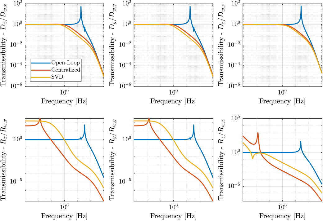
  legend('Control OFF','Decentralized control','Centralized control','SVD control','SVD control real appr.');

  figure
  bodemag(system_dec([7 9],4:6),CL_dec([7 9],4:6),CL_cen([7 9],4:6),CL_svd([7 9],4:6),CL_svd_real([7 9],4:6),P);
  title('Transmissibility from half sum and half difference in the X direction');
  legend('Control OFF','Decentralized control','Centralized control','SVD control','SVD control real appr.');

  figure
  bodemag(system_dec([8 10],4:6),CL_dec([8 10],4:6),CL_cen([8 10],4:6),CL_svd([8 10],4:6),CL_svd_real([8 10],4:6),P);
  title('Transmissibility from half sum and half difference in the Z direction');
  legend('Control OFF','Decentralized control','Centralized control','SVD control','SVD control real appr.');

Greshgorin radius

  system_dec_freq = freqresp(system_dec,w);
  x1 = zeros(1,length(w));
  z1 = zeros(1,length(w));
  x2 = zeros(1,length(w));
  S1 = zeros(1,length(w));
  S2 = zeros(1,length(w));
  S3 = zeros(1,length(w));

  for t = 1:length(w)
      x1(t) = (abs(system_dec_freq(1,2,t))+abs(system_dec_freq(1,3,t)))/abs(system_dec_freq(1,1,t));
      z1(t) = (abs(system_dec_freq(2,1,t))+abs(system_dec_freq(2,3,t)))/abs(system_dec_freq(2,2,t));
      x2(t) = (abs(system_dec_freq(3,1,t))+abs(system_dec_freq(3,2,t)))/abs(system_dec_freq(3,3,t));
      system_svd = pinv(Ureal)*system_dec_freq(1:4,1:3,t)*pinv(Vreal');
      S1(t) = (abs(system_svd(1,2))+abs(system_svd(1,3)))/abs(system_svd(1,1));
      S2(t) = (abs(system_svd(2,1))+abs(system_svd(2,3)))/abs(system_svd(2,2));
      S2(t) = (abs(system_svd(3,1))+abs(system_svd(3,2)))/abs(system_svd(3,3));
  end

  limit = 0.5*ones(1,length(w));

  figure
  loglog(w./(2*pi),x1,w./(2*pi),z1,w./(2*pi),x2,w./(2*pi),limit,'--');
  legend('x_1','z_1','x_2','Limit');
  xlabel('Frequency [Hz]');
  ylabel('Greshgorin radius [-]');

  figure
  loglog(w./(2*pi),S1,w./(2*pi),S2,w./(2*pi),S3,w./(2*pi),limit,'--');
  legend('S1','S2','S3','Limit');
  xlabel('Frequency [Hz]');
  ylabel('Greshgorin radius [-]');
  % set(gcf,'color','w')

Injecting ground motion in the system to have the output

  Fr = logspace(-2,3,1e3);
  w=2*pi*Fr*1i;
  %fit of the ground motion data in m/s^2/rtHz
  Fr_ground_x = [0.07 0.1 0.15 0.3 0.7 0.8 0.9 1.2 5 10];
  n_ground_x1 = [4e-7 4e-7 2e-6 1e-6 5e-7 5e-7 5e-7 1e-6 1e-5 3.5e-5];
  Fr_ground_v = [0.07 0.08 0.1 0.11 0.12 0.15 0.25 0.6 0.8 1 1.2 1.6 2 6 10];
  n_ground_v1 = [7e-7 7e-7 7e-7 1e-6 1.2e-6 1.5e-6 1e-6 9e-7 7e-7 7e-7 7e-7 1e-6 2e-6 1e-5 3e-5];

  n_ground_x = interp1(Fr_ground_x,n_ground_x1,Fr,'linear');
  n_ground_v = interp1(Fr_ground_v,n_ground_v1,Fr,'linear');
  % figure
  % loglog(Fr,abs(n_ground_v),Fr_ground_v,n_ground_v1,'*');
  % xlabel('Frequency [Hz]');ylabel('ASD [m/s^2 /rtHz]');
  % return

  %converting into PSD
  n_ground_x = (n_ground_x).^2;
  n_ground_v = (n_ground_v).^2;

  %Injecting ground motion in the system and getting the outputs
  system_dec_f = (freqresp(system_dec,abs(w)));
  PHI = zeros(size(Fr,2),12,12);
  for p = 1:size(Fr,2)
      Sw=zeros(6,6);
      Iact = zeros(3,3);
      Sw(4,4) = n_ground_x(p);
      Sw(5,5) = n_ground_v(p);
      Sw(6,6) = n_ground_v(p);
      Sw(1:3,1:3) = Iact;
      PHI(p,:,:) = (system_dec_f(:,:,p))*Sw(:,:)*(system_dec_f(:,:,p))';
  end
  x1 = PHI(:,1,1);
  z1 = PHI(:,2,2);
  x2 = PHI(:,3,3);
  z2 = PHI(:,4,4);
  wx = PHI(:,5,5);
  wz = PHI(:,6,6);
  x12 = PHI(:,1,3);
  z12 = PHI(:,2,4);
  PHIwx = PHI(:,1,5);
  PHIwz = PHI(:,2,6);
  xsum = PHI(:,7,7);
  zsum = PHI(:,8,8);
  xdelta = PHI(:,9,9);
  zdelta = PHI(:,10,10);
  rot = PHI(:,11,11);

Gravimeter - Functions

align

<<sec:align>>

This Matlab function is accessible here.

  function [A] = align(V)
  %A!ALIGN(V) returns a constat matrix A which is the real alignment of the
  %INVERSE of the complex input matrix V
  %from Mohit slides

      if (nargin ==0) || (nargin > 1)
          disp('usage: mat_inv_real = align(mat)')
          return
      end

      D = pinv(real(V'*V));
      A = D*real(V'*diag(exp(1i * angle(diag(V*D*V.'))/2)));


  end

pzmap_testCL

<<sec:pzmap_testCL>>

This Matlab function is accessible here.

  function [] = pzmap_testCL(system,H,gain,feedin,feedout)
  % evaluate and plot the pole-zero map for the closed loop system for
  % different values of the gain

      [~, n] = size(gain);
      [m1, n1, ~] = size(H);
      [~,n2] = size(feedin);

      figure
      for i = 1:n
          %     if n1 == n2
          system_CL = feedback(system,gain(i)*H,feedin,feedout);

          [P,Z] = pzmap(system_CL);
          plot(real(P(:)),imag(P(:)),'x',real(Z(:)),imag(Z(:)),'o');hold on
          xlabel('Real axis (s^{-1})');ylabel('Imaginary Axis (s^{-1})');
          %         clear P Z
          %     else
          %         system_CL = feedback(system,gain(i)*H(:,1+(i-1)*m1:m1+(i-1)*m1),feedin,feedout);
          %
          %         [P,Z] = pzmap(system_CL);
          %         plot(real(P(:)),imag(P(:)),'x',real(Z(:)),imag(Z(:)),'o');hold on
          %         xlabel('Real axis (s^{-1})');ylabel('Imaginary Axis (s^{-1})');
          %         clear P Z
          %     end
      end
      str = {strcat('gain = ' , num2str(gain(1)))};  % at the end of first loop, z being loop output
      str = [str , strcat('gain = ' , num2str(gain(1)))]; % after 2nd loop
      for i = 2:n
          str = [str , strcat('gain = ' , num2str(gain(i)))]; % after 2nd loop
          str = [str , strcat('gain = ' , num2str(gain(i)))]; % after 2nd loop
      end
      legend(str{:})
  end

Stewart Platform - Simscape Model

Introduction   ignore

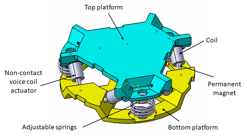
In this analysis, we wish to applied SVD control to the Stewart Platform shown in Figure fig:SP_assembly.

Stewart Platform CAD View

The analysis of the SVD control applied to the Stewart platform is performed in the following sections:

• Section sec:stewart_simscape: The parameters of the Simscape model of the Stewart platform are defined
• Section sec:stewart_identification: The plant is identified from the Simscape model and the centralized plant is computed thanks to the Jacobian
• Section sec:stewart_dynamics: The identified Dynamics is shown
• Section sec:stewart_real_approx: A real approximation of the plant is computed for further decoupling using the Singular Value Decomposition (SVD)
• Section sec:stewart_svd_decoupling: The decoupling is performed thanks to the SVD. The effectiveness of the decoupling is verified using the Gershorin Radii
• Section sec:stewart_decoupled_plant: The dynamics of the decoupled plant is shown
• Section sec:stewart_diagonal_control: A diagonal controller is defined to control the decoupled plant
• Section sec:stewart_closed_loop_results: Finally, the closed loop system properties are studied

Simscape Model - Parameters

<<sec:stewart_simscape>>

  open('drone_platform.slx');

Definition of spring parameters

  kx = 0.5*1e3/3; % [N/m]
  ky = 0.5*1e3/3;
  kz = 1e3/3;

  cx = 0.025; % [Nm/rad]
  cy = 0.025;
  cz = 0.025;

Gravity:

  g = 0;

We load the Jacobian (previously computed from the geometry).

  load('./jacobian.mat', 'Aa', 'Ab', 'As', 'l', 'J');

Identification of the plant

<<sec:stewart_identification>>

The dynamics is identified from forces applied by each legs to the measured acceleration of the top platform.

  %% Name of the Simulink File
  mdl = 'drone_platform';

  %% Input/Output definition
  clear io; io_i = 1;
  io(io_i) = linio([mdl, '/Dw'],              1, 'openinput');  io_i = io_i + 1;
  io(io_i) = linio([mdl, '/u'],               1, 'openinput');  io_i = io_i + 1;
  io(io_i) = linio([mdl, '/Inertial Sensor'], 1, 'openoutput'); io_i = io_i + 1;

  G = linearize(mdl, io);
  G.InputName  = {'Dwx', 'Dwy', 'Dwz', 'Rwx', 'Rwy', 'Rwz', ...
                  'F1', 'F2', 'F3', 'F4', 'F5', 'F6'};
  G.OutputName = {'Ax', 'Ay', 'Az', 'Arx', 'Ary', 'Arz'};

There are 24 states (6dof for the bottom platform + 6dof for the top platform).

  size(G)

State-space model with 6 outputs, 12 inputs, and 24 states.

The "centralized" plant $\bm{G}_x$ is now computed (Figure fig:centralized_control).

Centralized control architecture

Thanks to the Jacobian, we compute the transfer functions in the inertial frame (transfer function from forces and torques applied to the top platform to the absolute acceleration of the top platform).

  Gx = G*blkdiag(eye(6), inv(J'));
  Gx.InputName  = {'Dwx', 'Dwy', 'Dwz', 'Rwx', 'Rwy', 'Rwz', ...
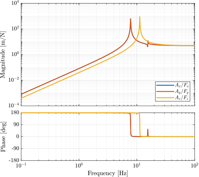
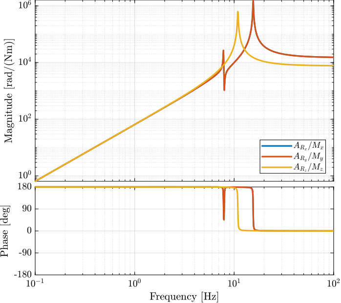
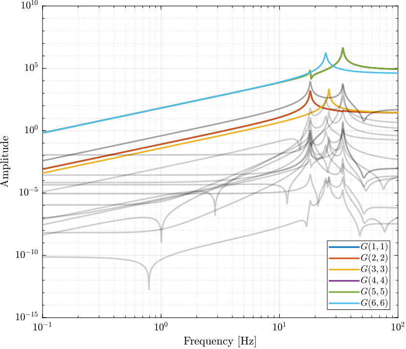
                   'Fx', 'Fy', 'Fz', 'Mx', 'My', 'Mz'};

Obtained Dynamics

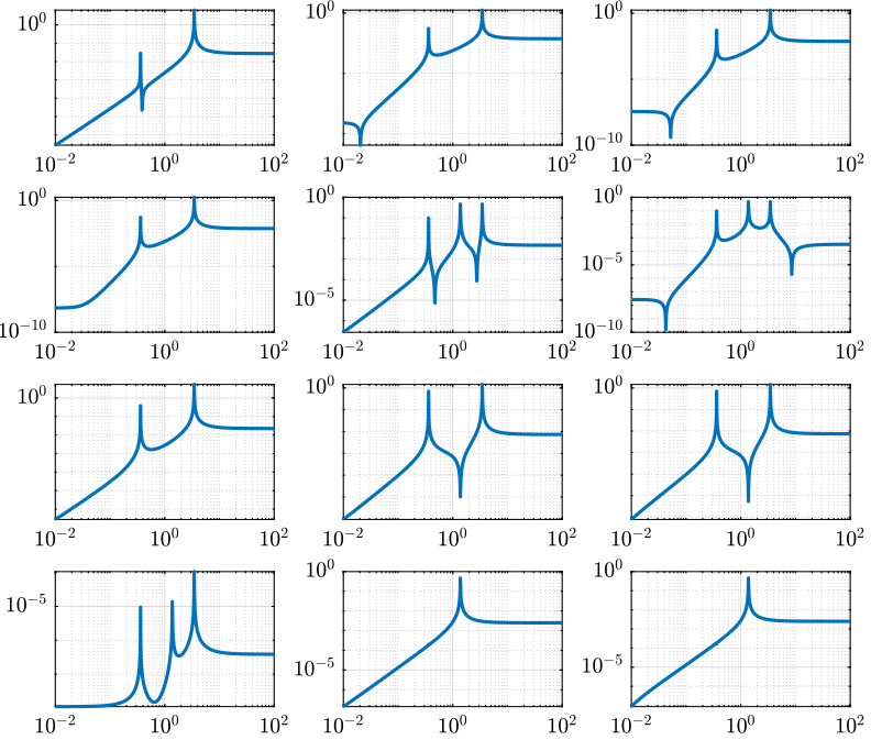
<<sec:stewart_dynamics>>

Stewart Platform Plant from forces applied by the legs to the acceleration of the platform

Stewart Platform Plant from torques applied by the legs to the angular acceleration of the platform

Real Approximation of $G$ at the decoupling frequency

<<sec:stewart_real_approx>>

Let's compute a real approximation of the complex matrix $H_1$ which corresponds to the the transfer function $G_c(j\omega_c)$ from forces applied by the actuators to the measured acceleration of the top platform evaluated at the frequency $\omega_c$.

  wc = 2*pi*30; % Decoupling frequency [rad/s]

  Gc = G({'Ax', 'Ay', 'Az', 'Arx', 'Ary', 'Arz'}, ...
         {'F1', 'F2', 'F3', 'F4', 'F5', 'F6'}); % Transfer function to find a real approximation

  H1 = evalfr(Gc, j*wc);

The real approximation is computed as follows:

  D = pinv(real(H1'*H1));
  H1 = inv(D*real(H1'*diag(exp(j*angle(diag(H1*D*H1.'))/2))));

4.4	-2.1	-2.1	4.4	-2.4	-2.4
-0.2	-3.9	3.9	0.2	-3.8	3.8
3.4	3.4	3.4	3.4	3.4	3.4
-367.1	-323.8	323.8	367.1	43.3	-43.3
-162.0	-237.0	-237.0	-162.0	398.9	398.9
220.6	-220.6	220.6	-220.6	220.6	-220.6

Real approximate of $G$ at the decoupling frequency $\omega_c$

Please not that the plant $G$ at $\omega_c$ is already an almost real matrix. This can be seen on the Bode plots where the phase is close to 1. This can be verified below where only the real value of $G(\omega_c)$ is shown

4.4	-2.1	-2.1	4.4	-2.4	-2.4
-0.2	-3.9	3.9	0.2	-3.8	3.8
3.4	3.4	3.4	3.4	3.4	3.4
-367.1	-323.8	323.8	367.1	43.3	-43.3
-162.0	-237.0	-237.0	-162.0	398.9	398.9
220.6	-220.6	220.6	-220.6	220.6	-220.6

Verification of the decoupling using the "Gershgorin Radii"

<<sec:stewart_svd_decoupling>>

First, the Singular Value Decomposition of $H_1$ is performed: \[ H_1 = U \Sigma V^H \]

  [U,S,V] = svd(H1);

Then, the "Gershgorin Radii" is computed for the plant $G_c(s)$ and the "SVD Decoupled Plant" $G_d(s)$: \[ G_d(s) = U^T G_c(s) V \]

This is computed over the following frequencies.

  freqs = logspace(-2, 2, 1000); % [Hz]

Gershgorin Radii for the coupled plant:

  Gr_coupled = zeros(length(freqs), size(Gc,2));

  H = abs(squeeze(freqresp(Gc, freqs, 'Hz')));
  for out_i = 1:size(Gc,2)
      Gr_coupled(:, out_i) = squeeze((sum(H(out_i,:,:)) - H(out_i,out_i,:))./H(out_i, out_i, :));
  end

Gershgorin Radii for the decoupled plant using SVD:

  Gd = U'*Gc*V;
  Gr_decoupled = zeros(length(freqs), size(Gd,2));

  H = abs(squeeze(freqresp(Gd, freqs, 'Hz')));
  for out_i = 1:size(Gd,2)
      Gr_decoupled(:, out_i) = squeeze((sum(H(out_i,:,:)) - H(out_i,out_i,:))./H(out_i, out_i, :));
  end

Gershgorin Radii for the decoupled plant using the Jacobian:

  Gj = Gc*inv(J');
  Gr_jacobian = zeros(length(freqs), size(Gj,2));

  H = abs(squeeze(freqresp(Gj, freqs, 'Hz')));

  for out_i = 1:size(Gj,2)
      Gr_jacobian(:, out_i) = squeeze((sum(H(out_i,:,:)) - H(out_i,out_i,:))./H(out_i, out_i, :));
  end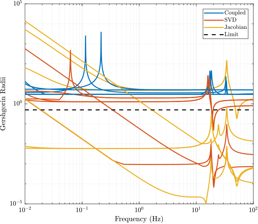

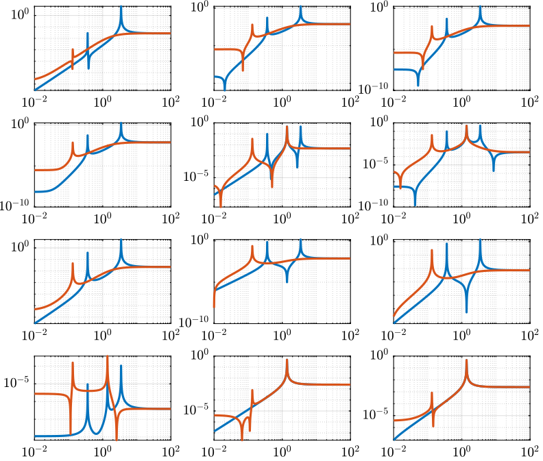
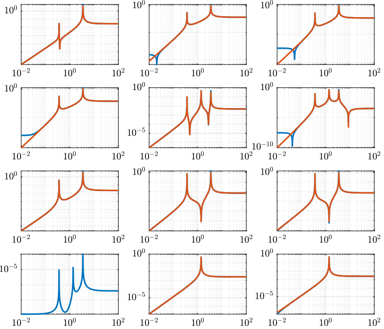
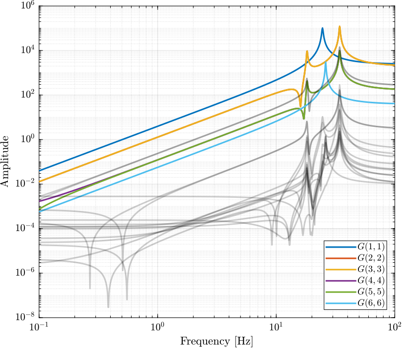
Gershgorin Radii of the Coupled and Decoupled plants

Decoupled Plant

<<sec:stewart_decoupled_plant>>

Let's see the bode plot of the decoupled plant $G_d(s)$. \[ G_d(s) = U^T G_c(s) V \]

Decoupled Plant using SVD

Decoupled Plant using the Jacobian

Diagonal Controller

<<sec:stewart_diagonal_control>>

The controller $K$ is a diagonal controller consisting a low pass filters with a crossover frequency $\omega_c$ and a DC gain $C_g$.

  wc = 2*pi*0.1; % Crossover Frequency [rad/s]
  C_g = 50; % DC Gain

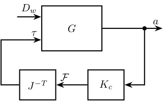
  K = eye(6)*C_g/(s+wc);

The control diagram for the centralized control is shown in Figure fig:centralized_control.

The controller $K_c$ is "working" in an cartesian frame. The Jacobian is used to convert forces in the cartesian frame to forces applied by the actuators.

Control Diagram for the Centralized control

The feedback system is computed as shown below.

  G_cen = feedback(G, inv(J')*K, [7:12], [1:6]);

The SVD control architecture is shown in Figure fig:svd_control. The matrices $U$ and $V$ are used to decoupled the plant $G$.

Control Diagram for the SVD control

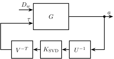
The feedback system is computed as shown below.

  G_svd = feedback(G, pinv(V')*K*pinv(U), [7:12], [1:6]);

Closed-Loop system Performances

<<sec:stewart_closed_loop_results>>

Let's first verify the stability of the closed-loop systems:

  isstable(G_cen)

ans =
  logical
   1

  isstable(G_svd)

ans =
  logical
   0

The obtained transmissibility in Open-loop, for the centralized control as well as for the SVD control are shown in Figure fig:stewart_platform_simscape_cl_transmissibility.

Obtained Transmissibility