24 KiB
Stewart Platform - Simscape Model
- Introduction
- Procedure
- Matlab Code
- initializeCubicConfiguration
- initializeGeneralConfiguration
- computeGeometricalProperties
- initializeMechanicalElements
- initializeSample
Introduction ignore
Stewart platforms are generated in multiple steps.
We define 4 important frames:
- $\{F\}$: Frame fixed to the Fixed base and located at the center of its bottom surface. This is used to fix the Stewart platform to some support.
- $\{M\}$: Frame fixed to the Moving platform and located at the center of its top surface. This is used to place things on top of the Stewart platform.
- $\{A\}$: Frame fixed to the fixed base. It defined the center of rotation of the moving platform.
- $\{B\}$: Frame fixed to the moving platform. The motion of the moving platforms and forces applied to it are defined with respect to this frame $\{B\}$.
Then, we define the location of the spherical joints:
- $\bm{a}_{i}$ are the position of the spherical joints fixed to the fixed base
- $\bm{b}_{i}$ are the position of the spherical joints fixed to the moving platform
We define the rest position of the Stewart platform:
- For simplicity, we suppose that the fixed base and the moving platform are parallel and aligned with the vertical axis at their rest position.
- Thus, to define the rest position of the Stewart platform, we just have to defined its total height $H$. $H$ corresponds to the distance from the bottom of the fixed base to the top of the moving platform.
From $\bm{a}_{i}$ and $\bm{b}_{i}$, we can determine the length and orientation of each strut:
- $l_{i}$ is the length of the strut
- ${}^{A}\hat{\bm{s}}_{i}$ is the unit vector align with the strut
The position of the Spherical joints can be done using various methods:
- Cubic configuration
- Geometrical
- Definition them by hand
- These methods should be easily scriptable and corresponds to specific functions that returns ${}^{F}\bm{a}_{i}$ and ${}^{M}\bm{b}_{i}$. The input of these functions are the parameters corresponding to the wanted geometry. We need also to know the height of the platform.
For Simscape, we need:
- The position of the frame $\{A\}$ with respect to the frame $\{F\}$: ${}^{F}\bm{O}_{A}$
- The position of the frame $\{B\}$ with respect to the frame $\{M\}$: ${}^{M}\bm{O}_{B}$
- The position and orientation of each spherical joint fixed to the fixed base: ${}^{F}\bm{a}_{i}$ and ${}^{F}\bm{R}_{a_{i}}$
- The position and orientation of each spherical joint fixed to the moving platform: ${}^{M}\bm{b}_{i}$ and ${}^{M}\bm{R}_{b_{i}}$
- The rest length of each strut: $l_{i}$
- The stiffness and damping of each actuator: $k_{i}$ and $c_{i}$
Procedure
The procedure is the following:
- Choose $H$
- Choose ${}^{F}\bm{O}_{A}$ and ${}^{M}\bm{O}_{B}$
- Choose $\bm{a}_{i}$ and $\bm{b}_{i}$, probably by specifying ${}^{F}\bm{a}_{i}$ and ${}^{M}\bm{b}_{i}$
- Choose $k_{i}$ and $c_{i}$
Matlab Code
Simscape Model
open('stewart_platform.slx')Define the Height of the Platform
  %% 1. Height of the platform. Location of {F} and {M}
  H = 90e-3; % [m]
  FO_M = [0; 0; H];
Define the location of {A} and {B}
  %% 2. Location of {A} and {B}
  FO_A = [0; 0; 100e-3] + FO_M;% [m,m,m]
  MO_B = [0; 0; 100e-3];% [m,m,m]
Define the position of $a_{i}$ and $b_{i}$
  %% 3. Position of ai and bi
  Fa = zeros(3, 6); % Fa_i is the i'th vector of Fa
  Mb = zeros(3, 6); % Mb_i is the i'th vector of Mb
Aa = Fa - repmat(FO_A, [1, 6]);
Bb = Mb - repmat(MO_B, [1, 6]);
Ab = Bb - repmat(-MO_B-FO_M+FO_A, [1, 6]);
Ba = Aa - repmat( MO_B+FO_M-FO_A, [1, 6]);
As = (Ab - Aa)./vecnorm(Ab - Aa); % As_i is the i'th vector of As
l = vecnorm(Ab - Aa);
Bs = (Bb - Ba)./vecnorm(Bb - Ba);
FRa = zeros(3,3,6);
MRb = zeros(3,3,6);
for i = 1:6
FRa(:,:,i) = [cross([0;1;0],As(:,i)) , cross(As(:,i), cross([0;1;0], As(:,i))) , As(:,i)];
FRa(:,:,i) = FRa(:,:,i)./vecnorm(FRa(:,:,i));
MRb(:,:,i) = [cross([0;1;0],Bs(:,i)) , cross(Bs(:,i), cross([0;1;0], Bs(:,i))) , Bs(:,i)];
MRb(:,:,i) = MRb(:,:,i)./vecnorm(MRb(:,:,i));
endDefine the dynamical properties of each strut
  %% 4. Stiffness and Damping of each strut
  Ki = 1e6*ones(6,1);
  Ci = 1e2*ones(6,1);
Old Introduction ignore
First, geometrical parameters are defined:
- ${}^A\bm{a}_i$ - Position of the joints fixed to the fixed base w.r.t $\{A\}$
- ${}^A\bm{b}_i$ - Position of the joints fixed to the mobile platform w.r.t $\{A\}$
- ${}^B\bm{b}_i$ - Position of the joints fixed to the mobile platform w.r.t $\{B\}$
- $H$ - Total height of the mobile platform
These parameter are enough to determine all the kinematic properties of the platform like the Jacobian, stroke, stiffness, …
These geometrical parameters can be generated using different functions: initializeCubicConfiguration for cubic configuration or initializeGeneralConfiguration for more general configuration.
A function computeGeometricalProperties is then used to compute:
- $\bm{J}_f$ - Jacobian matrix for the force location
- $\bm{J}_d$ - Jacobian matrix for displacement estimation
- $\bm{R}_m$ - Rotation matrices to position the leg vectors
Then, geometrical parameters are computed for all the mechanical elements with the function initializeMechanicalElements:
-
Shape of the platforms
- External Radius
- Internal Radius
- Density
- Thickness
-
Shape of the Legs
- Radius
- Size of ball joint
- Density
Other Parameters are defined for the Simscape simulation:
- Sample mass, volume and position (
initializeSamplefunction) - Location of the inertial sensor
- Location of the point for the differential measurements
- Location of the Jacobian point for velocity/displacement computation
Cubic Configuration
To define the cubic configuration, we need to define 4 parameters:
- The size of the cube
- The location of the cube
- The position of the plane joint the points $a_{i}$
- The position of the plane joint the points $b_{i}$
To do so, we specify the following parameters:
- $H_{C}$ the height of the useful part of the cube
- ${}^{F}O_{C}$ the position of the center of the cube with respect to $\{F\}$
- ${}^{F}H_{A}$: the height of the plane joining the points $a_{i}$ with respect to the frame $\{F\}$
- ${}^{M}H_{B}$: the height of the plane joining the points $b_{i}$ with respect to the frame $\{B\}$
We define the parameters
  Hc = 60e-3; % [m]
  FOc = 50e-3; % [m]
  FHa = 15e-3; % [m]
  MHb = 15e-3; % [m]
We define the useful points of the cube with respect to the Cube's center. ${}^{C}C$ are the 6 vertices of the cubes expressed in a frame {C} which is located at the center of the cube and aligned with {F} and {M}.
  sx = [ 2; -1; -1];
  sy = [ 0;  1; -1];
  sz = [ 1;  1;  1];

  R = [sx, sy, sz]./vecnorm([sx, sy, sz]);

  L = Hc*sqrt(3);

  Cc = R'*[[0;0;L],[L;0;L],[L;0;0],[L;L;0],[0;L;0],[0;L;L]] - [0;0;1.5*Hc];

  CCf = [Cc(:,1), Cc(:,3), Cc(:,3), Cc(:,5), Cc(:,5), Cc(:,1)]; % CCf(:,i) corresponds to the bottom cube's vertice corresponding to the i'th leg
  CCm = [Cc(:,2), Cc(:,2), Cc(:,4), Cc(:,4), Cc(:,6), Cc(:,6)]; % CCm(:,i) corresponds to the top cube's vertice corresponding to the i'th leg
We can compute the vector of each leg ${}^{C}\hat{\bm{s}}_{i}$ (unit vector from ${}^{C}C_{f}$ to ${}^{C}C_{m}$).
CSi = (CCm - CCf)./vecnorm(CCm - CCf);We now which to compute the position of the joints $a_{i}$ and $b_{i}$.
  Fa = zeros(3, 6); % Fa_i is the i'th vector of Fa
  Mb = zeros(3, 6); % Mb_i is the i'th vector of Mb
Fa = CCf + [0; 0; FOc] + ((FHa-(FOc-Hc/2))./CSi(3,:)).*CSi;
Mb = CCf + [0; 0; FOc-H] + ((H-MHb-(FOc-Hc/2))./CSi(3,:)).*CSi; % TODOinitializeCubicConfiguration
<<sec:initializeCubicConfiguration>>
Function description
function [stewart] = initializeCubicConfiguration(opts_param)Optional Parameters
Default values for opts.
  opts = struct(...
      'H_tot', 90,  ... % Total height of the Hexapod [mm]
      'L',     110, ... % Size of the Cube [mm]
      'H',     40,  ... % Height between base joints and platform joints [mm]
      'H0',    75   ... % Height between the corner of the cube and the plane containing the base joints [mm]
      );
Populate opts with input parameters
  if exist('opts_param','var')
      for opt = fieldnames(opts_param)'
          opts.(opt{1}) = opts_param.(opt{1});
      end
  end
Cube Creation
  points = [0, 0, 0; ...
            0, 0, 1; ...
            0, 1, 0; ...
            0, 1, 1; ...
            1, 0, 0; ...
            1, 0, 1; ...
            1, 1, 0; ...
            1, 1, 1];
  points = opts.L*points;
We create the rotation matrix to rotate the cube
  sx = cross([1, 1, 1], [1 0 0]);
  sx = sx/norm(sx);

  sy = -cross(sx, [1, 1, 1]);
  sy = sy/norm(sy);

  sz = [1, 1, 1];
  sz = sz/norm(sz);

  R = [sx', sy', sz']';
We use to rotation matrix to rotate the cube
  cube = zeros(size(points));
  for i = 1:size(points, 1)
    cube(i, :) = R * points(i, :)';
  end
Vectors of each leg
  leg_indices = [3, 4; ...
                 2, 4; ...
                 2, 6; ...
                 5, 6; ...
                 5, 7; ...
                 3, 7];
Vectors are:
  legs = zeros(6, 3);
  legs_start = zeros(6, 3);

  for i = 1:6
    legs(i, :) = cube(leg_indices(i, 2), :) - cube(leg_indices(i, 1), :);
    legs_start(i, :) = cube(leg_indices(i, 1), :);
  end
Verification of Height of the Stewart Platform
If the Stewart platform is not contained in the cube, throw an error.
  Hmax = cube(4, 3) - cube(2, 3);
  if opts.H0 < cube(2, 3)
    error(sprintf('H0 is not high enought. Minimum H0 = %.1f', cube(2, 3)));
  else if opts.H0 + opts.H > cube(4, 3)
    error(sprintf('H0+H is too high. Maximum H0+H = %.1f', cube(4, 3)));
    error('H0+H is too high');
  end
Determinate the location of the joints
We now determine the location of the joints on the fixed platform w.r.t the fixed frame $\{A\}$. $\{A\}$ is fixed to the bottom of the base.
  Aa = zeros(6, 3);
  for i = 1:6
    t = (opts.H0-legs_start(i, 3))/(legs(i, 3));
    Aa(i, :) = legs_start(i, :) + t*legs(i, :);
  end
And the location of the joints on the mobile platform with respect to $\{A\}$.
  Ab = zeros(6, 3);
  for i = 1:6
    t = (opts.H0+opts.H-legs_start(i, 3))/(legs(i, 3));
    Ab(i, :) = legs_start(i, :) + t*legs(i, :);
  end
And the location of the joints on the mobile platform with respect to $\{B\}$.
  Bb = zeros(6, 3);
  Bb = Ab - (opts.H0 + opts.H_tot/2 + opts.H/2)*[0, 0, 1];
h = opts.H0 + opts.H/2 - opts.H_tot/2;
Aa = Aa - h*[0, 0, 1];
Ab = Ab - h*[0, 0, 1];Returns Stewart Structure
  stewart = struct();
  stewart.Aa = Aa;
  stewart.Ab = Ab;
  stewart.Bb = Bb;
  stewart.H_tot = opts.H_tot;
end
initializeGeneralConfiguration
Function description
The initializeGeneralConfiguration function takes one structure that contains configurations for the hexapod and returns one structure representing the Hexapod.
function [stewart] = initializeGeneralConfiguration(opts_param)Optional Parameters
Default values for opts.
  opts = struct(...
      'H_tot',   90, ... % Height of the platform [mm]
      'H_joint', 15, ... % Height of the joints [mm]
      'H_plate', 10, ... % Thickness of the fixed and mobile platforms [mm]
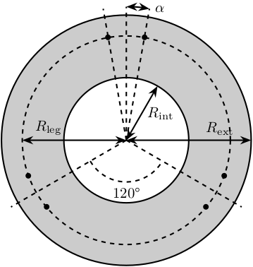
      'R_bot',  100, ... % Radius where the legs articulations are positionned [mm]
      'R_top',  80,  ... % Radius where the legs articulations are positionned [mm]
      'a_bot',  10,  ... % Angle Offset [deg]
      'a_top',  40,  ... % Angle Offset [deg]
      'da_top', 0    ... % Angle Offset from 0 position [deg]
      );
Populate opts with input parameters
  if exist('opts_param','var')
      for opt = fieldnames(opts_param)'
          opts.(opt{1}) = opts_param.(opt{1});
      end
endCompute Aa and Ab
We compute $[a_1, a_2, a_3, a_4, a_5, a_6]^T$ and $[b_1, b_2, b_3, b_4, b_5, b_6]^T$.
  Aa = zeros(6, 3); % [mm]
  Ab = zeros(6, 3); % [mm]
  Bb = zeros(6, 3); % [mm]
for i = 1:3
Aa(2*i-1,:) = [opts.R_bot*cos( pi/180*(120*(i-1) - opts.a_bot) ), ...
opts.R_bot*sin( pi/180*(120*(i-1) - opts.a_bot) ), ...
opts.H_plate+opts.H_joint];
Aa(2*i,:) = [opts.R_bot*cos( pi/180*(120*(i-1) + opts.a_bot) ), ...
opts.R_bot*sin( pi/180*(120*(i-1) + opts.a_bot) ), ...
opts.H_plate+opts.H_joint];
Ab(2*i-1,:) = [opts.R_top*cos( pi/180*(120*(i-1) + opts.da_top - opts.a_top) ), ...
opts.R_top*sin( pi/180*(120*(i-1) + opts.da_top - opts.a_top) ), ...
opts.H_tot - opts.H_plate - opts.H_joint];
Ab(2*i,:) = [opts.R_top*cos( pi/180*(120*(i-1) + opts.da_top + opts.a_top) ), ...
opts.R_top*sin( pi/180*(120*(i-1) + opts.da_top + opts.a_top) ), ...
opts.H_tot - opts.H_plate - opts.H_joint];
end
Bb = Ab - opts.H_tot*[0,0,1];Returns Stewart Structure
  stewart = struct();
  stewart.Aa = Aa;
  stewart.Ab = Ab;
  stewart.Bb = Bb;
  stewart.H_tot = opts.H_tot;
end
computeGeometricalProperties
Function description
function [stewart] = computeGeometricalProperties(stewart, opts_param)Optional Parameters
Default values for opts.
  opts = struct(...
      'Jd_pos', [0, 0, 30], ... % Position of the Jacobian for displacement estimation from the top of the mobile platform [mm]
      'Jf_pos', [0, 0, 30]  ... % Position of the Jacobian for force location from the top of the mobile platform [mm]
      );
Populate opts with input parameters
  if exist('opts_param','var')
      for opt = fieldnames(opts_param)'
          opts.(opt{1}) = opts_param.(opt{1});
      end
  end
Rotation matrices
We initialize $l_i$ and $\hat{s}_i$
  leg_length = zeros(6, 1); % [mm]
  leg_vectors = zeros(6, 3);
We compute $b_i - a_i$, and then:
\begin{align*} l_i &= \left|b_i - a_i\right| \\ \hat{s}_i &= \frac{b_i - a_i}{l_i} \end{align*} legs = stewart.Ab - stewart.Aa;
for i = 1:6
leg_length(i) = norm(legs(i,:));
leg_vectors(i,:) = legs(i,:) / leg_length(i);
endWe compute rotation matrices to have the orientation of the legs. The rotation matrix transforms the $z$ axis to the axis of the leg. The other axis are not important here.
  stewart.Rm = struct('R', eye(3));

  for i = 1:6
    sx = cross(leg_vectors(i,:), [1 0 0]);
    sx = sx/norm(sx);

    sy = -cross(sx, leg_vectors(i,:));
    sy = sy/norm(sy);

    sz = leg_vectors(i,:);
    sz = sz/norm(sz);

    stewart.Rm(i).R = [sx', sy', sz'];
  end
Jacobian matrices
Compute Jacobian Matrix
  Jd = zeros(6);

  for i = 1:6
    Jd(i, 1:3) = leg_vectors(i, :);
    Jd(i, 4:6) = cross(0.001*(stewart.Bb(i, :) - opts.Jd_pos), leg_vectors(i, :));
  end

  stewart.Jd = Jd;
  stewart.Jd_inv = inv(Jd);
Jf = zeros(6);
for i = 1:6
Jf(i, 1:3) = leg_vectors(i, :);
Jf(i, 4:6) = cross(0.001*(stewart.Bb(i, :) - opts.Jf_pos), leg_vectors(i, :));
end
stewart.Jf = Jf;
stewart.Jf_inv = inv(Jf); endinitializeMechanicalElements
Function description
function [stewart] = initializeMechanicalElements(stewart, opts_param)Optional Parameters
Default values for opts.
  opts = struct(...
      'thickness', 10, ... % Thickness of the base and platform [mm]
      'density',   1000, ... % Density of the material used for the hexapod [kg/m3]
      'k_ax',      1e8, ... % Stiffness of each actuator [N/m]
      'c_ax',      1000, ... % Damping of each actuator [N/(m/s)]
      'stroke',    50e-6  ... % Maximum stroke of each actuator [m]
      );
Populate opts with input parameters
  if exist('opts_param','var')
      for opt = fieldnames(opts_param)'
          opts.(opt{1}) = opts_param.(opt{1});
      end
  end
Bottom Plate

The bottom plate structure is initialized.
BP = struct();We defined its internal radius (if there is a hole in the bottom plate) and its outer radius.
  BP.Rint = 0;   % Internal Radius [mm]
  BP.Rext = 150; % External Radius [mm]
We define its thickness.
BP.H = opts.thickness; % Thickness of the Bottom Plate [mm]We defined the density of the material of the bottom plate.
BP.density = opts.density; % Density of the material [kg/m3]And its color.
BP.color = [0.7 0.7 0.7]; % Color [RGB]Then the profile of the bottom plate is computed and will be used by Simscape
BP.shape = [BP.Rint BP.H; BP.Rint 0; BP.Rext 0; BP.Rext BP.H]; % [mm]The structure is added to the stewart structure
stewart.BP = BP;Top Plate
The top plate structure is initialized.
TP = struct();We defined the internal and external radius of the top plate.
  TP.Rint = 0;   % [mm]
  TP.Rext = 100; % [mm]
The thickness of the top plate.
TP.H = 10; % [mm]The density of its material.
TP.density = opts.density; % Density of the material [kg/m3]Its color.
TP.color = [0.7 0.7 0.7]; % Color [RGB]Then the shape of the top plate is computed
TP.shape = [TP.Rint TP.H; TP.Rint 0; TP.Rext 0; TP.Rext TP.H];The structure is added to the stewart structure
stewart.TP = TP;Legs

The leg structure is initialized.
Leg = struct();The maximum Stroke of each leg is defined.
Leg.stroke = opts.stroke; % [m]The stiffness and damping of each leg are defined
  Leg.k_ax = opts.k_ax; % Stiffness of each leg [N/m]
  Leg.c_ax = opts.c_ax; % Damping of each leg [N/(m/s)]
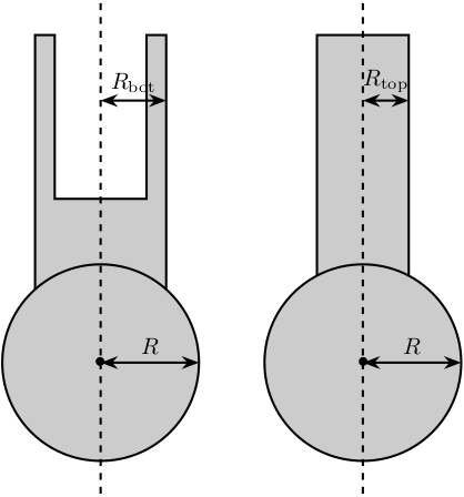
The radius of the legs are defined
  Leg.Rtop = 10; % Radius of the cylinder of the top part of the leg[mm]
  Leg.Rbot = 12; % Radius of the cylinder of the bottom part of the leg [mm]
The density of its material.
Leg.density = opts.density; % Density of the material used for the legs [kg/m3]Its color.
Leg.color = [0.5 0.5 0.5]; % Color of the top part of the leg [RGB]The radius of spheres representing the ball joints are defined.
Leg.R = 1.3*Leg.Rbot; % Size of the sphere at the extremity of the leg [mm]We estimate the length of the legs.
  legs = stewart.Ab - stewart.Aa;
  Leg.lenght = norm(legs(1,:))/1.5;
Then the shape of the bottom leg is estimated
  Leg.shape.bot = ...
      [0        0; ...
       Leg.Rbot 0; ...
       Leg.Rbot Leg.lenght; ...
       Leg.Rtop Leg.lenght; ...
       Leg.Rtop 0.2*Leg.lenght; ...
       0        0.2*Leg.lenght];
The structure is added to the stewart structure
stewart.Leg = Leg;Ball Joints

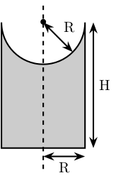
SP is the structure representing the support for the ball joints at the extremity of each leg.
The SP structure is initialized.
SP = struct();We can define its rotational stiffness and damping. For now, we use perfect joints.
  SP.k = 0; % [N*m/deg]
  SP.c = 0; % [N*m/deg]
Its height is defined
SP.H = stewart.Aa(1, 3) - BP.H; % [mm]Its radius is based on the radius on the sphere at the end of the legs.
SP.R = Leg.R; % [mm] SP.section = [0 SP.H-SP.R;
0 0;
SP.R 0;
SP.R SP.H];The density of its material is defined.
SP.density = opts.density; % [kg/m^3]Its color is defined.
SP.color = [0.7 0.7 0.7]; % [RGB]The structure is added to the Hexapod structure
stewart.SP = SP;initializeSample
Function description
function [] = initializeSample(opts_param)Optional Parameters
Default values for opts.
  sample = struct( ...
      'radius',     100, ... % radius of the cylinder [mm]
      'height',     100, ... % height of the cylinder [mm]
      'mass',       10,  ... % mass of the cylinder [kg]
      'measheight', 50, ... % measurement point z-offset [mm]
      'offset',     [0, 0, 0],   ... % offset position of the sample [mm]
      'color',      [0.9 0.1 0.1] ...
      );
Populate opts with input parameters
  if exist('opts_param','var')
      for opt = fieldnames(opts_param)'
          sample.(opt{1}) = opts_param.(opt{1});
      end
  end
Save the Sample structure
save('./mat/sample.mat', 'sample'); end