stewart-simscape/simscape-model.org

Stewart Platform - Simscape Model

• Function description and arguments
• Initialization of the stewart structure
• Bottom Plate
• Top Plate
• Legs
• Ball Joints
• More parameters are initialized
• Save the Stewart Structure
• initializeParameters Function
• initializeSample

Function description and arguments

The initializeHexapod function takes one structure that contains configurations for the hexapod and returns one structure representing the hexapod.

  function [stewart] = initializeHexapod(opts_param)

Default values for opts.

  opts = struct(...
      'height',  90,    ... % Height of the platform [mm]
      'density', 8000,  ... % Density of the material used for the hexapod [kg/m3]
      'k_ax',    1e8,   ... % Stiffness of each actuator [N/m]
      'c_ax',    1000,   ... % Damping of each actuator [N/(m/s)]
      'stroke',  50e-6, ... % Maximum stroke of each actuator [m]
      'name',    'stewart' ... % Name of the file
      );

Populate opts with input parameters

  if exist('opts_param','var')
      for opt = fieldnames(opts_param)'
          opts.(opt{1}) = opts_param.(opt{1});
      end
  end

Initialization of the stewart structure

We initialize the Stewart structure

  stewart = struct();

And we defined its total height.

  stewart.H = opts.height; % [mm]

Bottom Plate

Schematic of the bottom plates with all the parameters

The bottom plate structure is initialized.

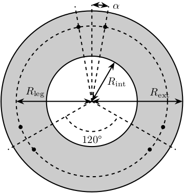
  BP = struct();

We defined its internal radius (if there is a hole in the bottom plate) and its outer radius.

  BP.Rint = 0;   % Internal Radius [mm]
  BP.Rext = 150; % External Radius [mm]

We define its thickness.

  BP.H = 10; % Thickness of the Bottom Plate [mm]

At which radius legs will be fixed and with that angle offset.

  BP.Rleg  = 100; % Radius where the legs articulations are positionned [mm]
  BP.alpha = 10;  % Angle Offset [deg]

We defined the density of the material of the bottom plate.

  BP.density = opts.density; % Density of the material [kg/m3]

And its color.

  BP.color = [0.7 0.7 0.7]; % Color [RGB]

Then the profile of the bottom plate is computed and will be used by Simscape

  BP.shape = [BP.Rint BP.H; BP.Rint 0; BP.Rext 0; BP.Rext BP.H]; % [mm]

The structure is added to the stewart structure

  stewart.BP = BP;

Top Plate

The top plate structure is initialized.

  TP = struct();

We defined the internal and external radius of the top plate.

  TP.Rint = 0;   % [mm]
  TP.Rext = 100; % [mm]

The thickness of the top plate.

  TP.H = 10; % [mm]

At which radius and angle are fixed the legs.

  TP.Rleg   = 100; % Radius where the legs articulations are positionned [mm]
  TP.alpha  = 20; % Angle [deg]
  TP.dalpha = 0; % Angle Offset from 0 position [deg]

The density of its material.

  TP.density = opts.density; % Density of the material [kg/m3]

Its color.

  TP.color = [0.7 0.7 0.7]; % Color [RGB]

Then the shape of the top plate is computed

  TP.shape = [TP.Rint TP.H; TP.Rint 0; TP.Rext 0; TP.Rext TP.H];

The structure is added to the stewart structure

  stewart.TP  = TP;

Legs

Schematic for the legs of the Stewart platform

The leg structure is initialized.

  Leg = struct();

The maximum Stroke of each leg is defined.

  Leg.stroke = opts.stroke; % [m]

The stiffness and damping of each leg are defined

  Leg.k_ax = opts.k_ax; % Stiffness of each leg [N/m]
  Leg.c_ax = opts.c_ax; % Damping of each leg [N/(m/s)]

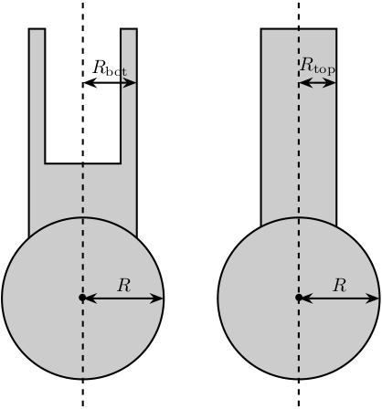
The radius of the legs are defined

  Leg.Rtop = 10; % Radius of the cylinder of the top part of the leg[mm]
  Leg.Rbot = 12; % Radius of the cylinder of the bottom part of the leg [mm]

The density of its material.

  Leg.density = opts.density; % Density of the material used for the legs [kg/m3]

Its color.

  Leg.color = [0.5 0.5 0.5]; % Color of the top part of the leg [RGB]

The radius of spheres representing the ball joints are defined.

  Leg.R = 1.3*Leg.Rbot; % Size of the sphere at the extremity of the leg [mm]

The structure is added to the stewart structure

  stewart.Leg = Leg;

Ball Joints

Schematic of the support for the ball joints

SP is the structure representing the support for the ball joints at the extremity of each leg.

The SP structure is initialized.

  SP = struct();

We can define its rotational stiffness and damping. For now, we use perfect joints.

  SP.k = 0; % [N*m/deg]
  SP.c = 0; % [N*m/deg]

Its height is defined

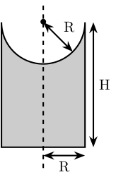
  SP.H = 15; % [mm]

Its radius is based on the radius on the sphere at the end of the legs.

  SP.R = Leg.R; % [mm]

  SP.section = [0    SP.H-SP.R;
                0    0;
                SP.R 0;
                SP.R SP.H];

The density of its material is defined.

  SP.density = opts.density; % [kg/m^3]

Its color is defined.

  SP.color = [0.7 0.7 0.7]; % [RGB]

The structure is added to the Hexapod structure

  stewart.SP  = SP;

More parameters are initialized

  stewart = initializeParameters(stewart);

Save the Stewart Structure

  save('./mat/stewart.mat', 'stewart')

initializeParameters Function

  function [stewart] = initializeParameters(stewart)

We first compute $[a_1, a_2, a_3, a_4, a_5, a_6]^T$ and $[b_1, b_2, b_3, b_4, b_5, b_6]^T$.

  stewart.Aa = zeros(6, 3); % [mm]
  stewart.Ab = zeros(6, 3); % [mm]
  stewart.Bb = zeros(6, 3); % [mm]

  for i = 1:3
      stewart.Aa(2*i-1,:) = [stewart.BP.Rleg*cos( pi/180*(120*(i-1) - stewart.BP.alpha) ), ...
                             stewart.BP.Rleg*sin( pi/180*(120*(i-1) - stewart.BP.alpha) ), ...
                             stewart.BP.H+stewart.SP.H];
      stewart.Aa(2*i,:)   = [stewart.BP.Rleg*cos( pi/180*(120*(i-1) + stewart.BP.alpha) ), ...
                             stewart.BP.Rleg*sin( pi/180*(120*(i-1) + stewart.BP.alpha) ), ...
                             stewart.BP.H+stewart.SP.H];

      stewart.Ab(2*i-1,:) = [stewart.TP.Rleg*cos( pi/180*(120*(i-1) + stewart.TP.dalpha - stewart.TP.alpha) ), ...
                             stewart.TP.Rleg*sin( pi/180*(120*(i-1) + stewart.TP.dalpha - stewart.TP.alpha) ), ...
                             stewart.H - stewart.TP.H - stewart.SP.H];
      stewart.Ab(2*i,:)   = [stewart.TP.Rleg*cos( pi/180*(120*(i-1) + stewart.TP.dalpha + stewart.TP.alpha) ), ...
                             stewart.TP.Rleg*sin( pi/180*(120*(i-1) + stewart.TP.dalpha + stewart.TP.alpha) ), ...
                             stewart.H - stewart.TP.H - stewart.SP.H];
  end
  stewart.Bb = stewart.Ab - stewart.H*[0,0,1];

Now, we compute the leg vectors $\hat{s}_i$ and leg position $l_i$: \[ b_i - a_i = l_i \hat{s}_i \]

We initialize $l_i$ and $\hat{s}_i$

  leg_length = zeros(6, 1); % [mm]
  leg_vectors = zeros(6, 3);

We compute $b_i - a_i$, and then:

\begin{align*} l_i &= \left|b_i - a_i\right| \\ \hat{s}_i &= \frac{b_i - a_i}{l_i} \end{align*}

  legs = stewart.Ab - stewart.Aa;

  for i = 1:6
      leg_length(i) = norm(legs(i,:));
      leg_vectors(i,:) = legs(i,:) / leg_length(i);
  end

Then the shape of the bottom leg is estimated

  stewart.Leg.lenght = leg_length(1)/1.5;
  stewart.Leg.shape.bot = ...
      [0                0; ...
       stewart.Leg.Rbot 0; ...
       stewart.Leg.Rbot stewart.Leg.lenght; ...
       stewart.Leg.Rtop stewart.Leg.lenght; ...
       stewart.Leg.Rtop 0.2*stewart.Leg.lenght; ...
       0                0.2*stewart.Leg.lenght];

We compute rotation matrices to have the orientation of the legs. The rotation matrix transforms the $z$ axis to the axis of the leg. The other axis are not important here.

  stewart.Rm = struct('R', eye(3));

  for i = 1:6
    sx = cross(leg_vectors(i,:), [1 0 0]);
    sx = sx/norm(sx);

    sy = -cross(sx, leg_vectors(i,:));
    sy = sy/norm(sy);

    sz = leg_vectors(i,:);
    sz = sz/norm(sz);

    stewart.Rm(i).R = [sx', sy', sz'];
  end

Compute Jacobian Matrix

  J = zeros(6);

  for i = 1:6
    J(i, 1:3) = leg_vectors(i, :);
    J(i, 4:6) = cross(0.001*(stewart.Ab(i, :)- stewart.H*[0,0,1]), leg_vectors(i, :));
  end

  stewart.J = J;
  stewart.Jinv = inv(J);

  stewart.K = stewart.Leg.k_ax*stewart.J'*stewart.J;

    end
  end

initializeSample

  function [] = initializeSample(opts_param)
  %% Default values for opts
      sample = struct( ...
          'radius',     100, ... % radius of the cylinder [mm]
          'height',     100, ... % height of the cylinder [mm]
          'mass',       10,  ... % mass of the cylinder [kg]
          'measheight', 50, ... % measurement point z-offset [mm]
          'offset',     [0, 0, 0],   ... % offset position of the sample [mm]
          'color',      [0.9 0.1 0.1] ...
          );

      %% Populate opts with input parameters
      if exist('opts_param','var')
          for opt = fieldnames(opts_param)'
              sample.(opt{1}) = opts_param.(opt{1});
          end
      end

      %% Save
      save('./mat/sample.mat', 'sample');
  end