spectral-analysis/index.org

Compute Spectral Densities of signals with Matlab

• Introduction
• Spectral Analysis - Basics
  • Introduction
  • PSD of ADC quantization noise
  • Sensitivity of the instrumentation
  • Convert the time domain from volts to velocity
  • Power Spectral Density and Amplitude Spectral Density
  • Modification of a signal's Power Spectral Density when going through an LTI system
  • From PSD of the velocity to the PSD of the displacement
  • Cumulative Power/Amplitude Spectrum
  • Add best practices from the Article and simple snippet that works
• Technique 1 : Approximation with a transfer function
  • Introduction
  • Signal's PSD
  • Transfer Function that approximate the ASD
  • Generated Time domain signal
  • Comparison of the Power Spectral Densities
  • Simulink
• Technique 2 : IFFT
  • Introduction
  • Signal's PSD
  • Algorithm
  • Obtained Time Domain Signal
  • PSD Comparison
• Compute the Noise level and Signal level from PSD
  • Introduction
  • Computation
• Bibliography

Introduction   ignore

This document presents the mathematics as well as the matlab scripts to do various spectral analysis on a measured signal.

Some matlab documentation about Spectral Analysis can be found here.

First, in section sec:spectral_analysis_basics, some basics of spectral analysis are presented.

In some cases, we want to generate a time domain signal with defined Power Spectral Density. Two methods are presented in sections sec:approximate_tf and sec:approximate_ifft.

Finally, some notes are done on how to compute the noise level and signal level from a given Power Spectral Density in section sec:compute_psd_levels.

Spectral Analysis - Basics

<<sec:spectral_analysis_basics>>

Introduction   ignore

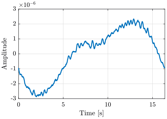
Typically this signal is coming from an inertial sensor, a force sensor or any other sensor.

We here take the example of a signal coming from a Geophone measurement the vertical velocity of the floor at the ESRF.

PSD of ADC quantization noise

This is taken from here.

Let's note:

• $q$ is the corresponding value in [V] of the least significant bit (LSB)
• $\Delta V$ is the full range of the ADC in [V]
• $n$ is the number of ADC's bits
• $f_s$ is the sample frequency in [Hz]

Let's suppose that the ADC is ideal. The only noise comes from the quantization error. Interestingly, the noise amplitude is uniformly distributed.

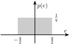
The quantization noise can take a value between $\pm q/2$, and the probability density function is constant in this range (i.e., it’s a uniform distribution). Since the integral of the probability density function is equal to one, its value will be $1/q$ for $-q/2 < e < q/2$ (Fig. fig:probability_density_function_adc).

Probability density function $p(e)$ of the ADC error $e$

Now, we can calculate the time average power of the quantization noise as

\begin{equation} P_q = \int_{-q/2}^{q/2} e^2 p(e) de = \frac{q^2}{12} \end{equation}

The other important parameter of a noise source is the power spectral density (PSD), which indicates how the noise power spreads in different frequency bands. To find the power spectral density, we need to calculate the Fourier transform of the autocorrelation function of the noise.

Assuming that the noise samples are not correlated with one another, we can approximate the autocorrelation function with a delta function in the time domain. Since the Fourier transform of a delta function is equal to one, the power spectral density will be frequency independent. Therefore, the quantization noise is white noise with total power equal to $P_q = \frac{q^2}{12}$.

Thus, the two-sided PSD (from $\frac{-f_s}{2}$ to $\frac{f_s}{2}$), we should divide the noise power $P_q$ by $f_s$:

\begin{equation} \int_{-f_s/2}^{f_s/2} \Gamma(f) d f = f_s \Gamma = \frac{q^2}{12} \end{equation}

Finally:

\begin{equation} \begin{align} \Gamma &= \frac{q^2}{12 f_s} \\ &= \frac{\left(\frac{\Delta V}{2^n}\right)^2}{12 f_s} \text{ in } \left[ \frac{V^2}{Hz} \right] \end{align} \end{equation}

Sensitivity of the instrumentation

The measured signal $x$ by the ADC is in Volts. The corresponding real velocity $v$ in m/s.

To obtain the real quantity as measured by the sensor, one have to know the sensitivity of the sensors and electronics used.

Schematic of the instrumentation used for the measurement

Convert the time domain from volts to velocity

Let's say, we know that the sensitivity of the geophone used is \[ G_g(s) = G_0 \frac{\frac{s}{2\pi f_0}}{1 + \frac{s}{2\pi f_0}} \quad \left[\frac{V}{m/s}\right] \]

  G0 = 88; % Sensitivity [V/(m/s)]
  f0 = 2; % Cut-off frequency [Hz]

  Gg = G0*(s/2/pi/f0)/(1+s/2/pi/f0);

And the gain of the amplifier is 1000: $G_m(s) = 1000$.

  Gm = 1000;

If ${G_m(s)}^{-1} {G_g(s)}^{-1}$ is proper, we can simulate this dynamical system to go from the voltage to the velocity units (figure fig:voltage_to_velocity).

  data = load('mat/data_028.mat', 'data'); data = data.data;

  t = data(:, 3); % [s]
  x = data(:, 1)-mean(data(:, 1)); % The offset if removed (coming from the voltage amplifier) [v]

  dt = t(2)-t(1); Fs = 1/dt;

Schematic of the instrumentation used for the measurement

We simulate this system with matlab:

  v = lsim(inv(Gg*Gm), x, t);

And we plot the obtained velocity

  figure;
  plot(t, v);
  xlabel("Time [s]"); ylabel("Velocity [m/s]");

  <<plt-matlab>>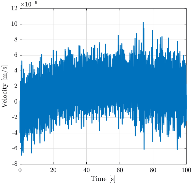

Measured Velocity

Power Spectral Density and Amplitude Spectral Density

We now have the velocity in the time domain: \[ v(t)\ [m/s] \]

To compute the Power Spectral Density (PSD): \[ S_v(f)\ \left[\frac{(m/s)^2}{Hz}\right] \]

To compute that with matlab, we use the pwelch function.

We first have to defined a window:

  win = hanning(ceil(10*Fs)); % 10s window

  [Sv, f] = pwelch(v, win, [], [], Fs);

  figure;
  loglog(f, Sv);
  xlabel('Frequency [Hz]');
  ylabel('Power Spectral Density $\left[\frac{(m/s)^2}{Hz}\right]$')

  <<plt-matlab>>

The Amplitude Spectral Density (ASD) is the square root of the Power Spectral Density:

Power Spectral Density of the measured velocity

\begin{equation} \Gamma_{vv}(f) = \sqrt{S_{vv}(f)} \quad \left[ \frac{m/s}{\sqrt{Hz}} \right] \end{equation}

  figure;
  loglog(f, sqrt(Sv));
  xlabel('Frequency [Hz]');
  ylabel('Amplitude Spectral Density $\left[\frac{m/s}{\sqrt{Hz}}\right]$')

  <<plt-matlab>>

Power Spectral Density of the measured velocity

Modification of a signal's Power Spectral Density when going through an LTI system

Schematic of the instrumentation used for the measurement

We can show that:

\begin{equation} S_{yy}(\omega) = \left|G(j\omega)\right|^2 S_{xx}(\omega) \end{equation}

And we also have:

\begin{equation} \Gamma_{yy}(\omega) = \left|G(j\omega)\right| \Gamma_{xx}(\omega) \end{equation}

From PSD of the velocity to the PSD of the displacement

Schematic of the instrumentation used for the measurement

The displacement is the integral of the velocity.

We then have that

\begin{equation} S_{xx}(\omega) = \left|\frac{1}{j \omega}\right|^2 S_{vv}(\omega) \end{equation}

Using a frequency variable in Hz:

\begin{equation} S_{xx}(f) = \left| \frac{1}{j 2\pi f} \right|^2 S_{vv}(f) \end{equation}

For the Amplitude Spectral Density:

\begin{equation} \Gamma_{xx}(f) = \frac{1}{2\pi f} \Gamma_{vv}(f) \end{equation}

\begin{equation} S_{xx}(\omega = 1) = S_{vv}(\omega = 1) \end{equation}

Now if we want to obtain the Power Spectral Density of the Position or Acceleration: For each frequency: \[ \left| \frac{d sin(2 \pi f t)}{dt} \right| = | 2 \pi f | \times | \cos(2\pi f t) | \]

\[ \left| \int_0^t sin(2 \pi f \tau) d\tau \right| = \left| \frac{1}{2 \pi f} \right| \times | \cos(2\pi f t) | \]

\[ ASD_x(f) = \frac{1}{2\pi f} ASD_v(f) \ \left[\frac{m}{\sqrt{Hz}}\right] \]

\[ ASD_a(f) = 2\pi f ASD_v(f) \ \left[\frac{m/s^2}{\sqrt{Hz}}\right] \] And we have \[ PSD_x(f) = {ASD_x(f)}^2 = \frac{1}{(2 \pi f)^2} {ASD_v(f)}^2 = \frac{1}{(2 \pi f)^2} PSD_v(f) \]

Note here that we always have \[ PSD_x \left(f = \frac{1}{2\pi}\right) = PSD_v \left(f = \frac{1}{2\pi}\right) = PSD_a \left(f = \frac{1}{2\pi}\right), \quad \frac{1}{2\pi} \approx 0.16 [Hz] \]

Cumulative Power/Amplitude Spectrum

If we want to compute the Cumulative Power Spectrum: \[ CPS_v(f) = \int_0^f PSD_v(\nu) d\nu \quad [(m/s)^2] \]

We can also want to integrate from high frequency to low frequency: \[ CPS_v(f) = \int_f^\infty PSD_v(\nu) d\nu \quad [(m/s)^2] \]

The Cumulative Amplitude Spectrum is then the square root of the Cumulative Power Spectrum: \[ CAS_v(f) = \sqrt{CPS_v(f)} = \sqrt{\int_f^\infty PSD_v(\nu) d\nu} \quad [m/s] \]

Then, we can obtain the Root Mean Square value of the velocity: \[ v_{\text{rms}} = CAS_v(0) \quad [m/s \ \text{rms}] \]

  figure;
  hold on;
  plot(f, cumtrapz(f, Sv));
  hold off;
  set(gca, 'xscale', 'log'); set(gca, 'yscale', 'log');
  xlabel('Frequency [Hz]'); ylabel('Cumulative Power Spectrum [$(m/s)^2$]')

In order to integrate from high frequency to low frequency:

  figure;
  hold on;
  plot(f, flip(-cumtrapz(flip(f), flip(Sv))));
  hold off;
  set(gca, 'xscale', 'log'); set(gca, 'yscale', 'log');
  xlabel('Frequency [Hz]'); ylabel('Cumulative Power Spectrum [$(m/s)^2$]')

TODO Add best practices from the Article and simple snippet that works

Technique 1 : Approximation with a transfer function

<<sec:approximate_tf>>

Introduction   ignore

Signal's PSD

We load the PSD of the signal we wish to replicate.

  load('./mat/dist_psd.mat', 'dist_f');

We remove the first value with very high PSD.

  dist_f.f = dist_f.f(3:end);
  dist_f.psd_gm = dist_f.psd_gm(3:end);

The PSD of the signal is shown on figure ref:fig:psd_ground_motion.

  <<plt-matlab>>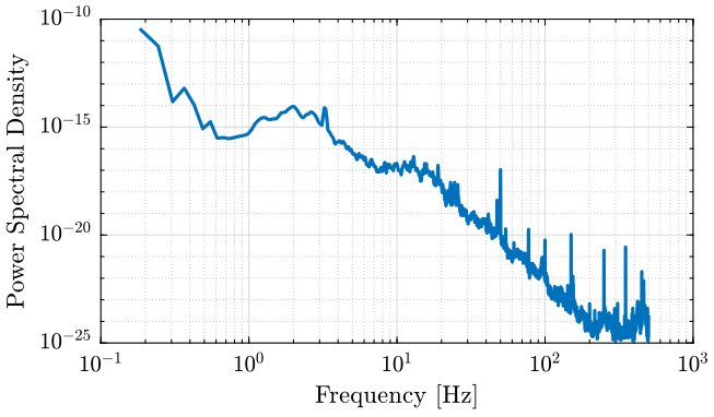

PSD of the signal (png, pdf)

Transfer Function that approximate the ASD

  G_gm = 0.002*(s^2 + 3.169*s + 27.74)/(s*(s+32.73)*(s+8.829)*(s+7.983)^2);

Generated Time domain signal

  Fs = 2*dist_f.f(end);
  Ts = 1/Fs;

  t = 0:Ts:500;
  u = sqrt(Fs/2)*randn(length(t), 1);

  u_o = lsim(G_gm, u, t);

  figure;
  plot(t, u_o);

Comparison of the Power Spectral Densities

  nx = length(u_o);
  na = 16;
  win = hanning(floor(nx/na));

  [pxx, f] = pwelch(u_o, win, 0, [], Fs);

Finally, we compare the PSD of the original signal and the obtained signal on figure ref:fig:psd_comparison.

Simulink

Simulink Schematic

The parameters for the Band-Limited White Noise are:

• Noise Power: 1

  nx = length(out.u_gm.Data);
  na = 8;
  win = hanning(floor(nx/na));

  [pxx, f] = pwelch(out.u_gm.Data, win, 0, [], 1e3);

Technique 2 : IFFT

<<sec:approximate_ifft>>

Introduction   ignore

The technique comes from cite:preumont94_random_vibrat_spect_analy (section 12.11).

Signal's PSD

We load the PSD of the signal we wish to replicate.

  load('./mat/dist_psd.mat', 'dist_f');

We remove the first value with very high PSD.

  dist_f.f = dist_f.f(3:end);
  dist_f.psd_gm = dist_f.psd_gm(3:end);

The PSD of the signal is shown on figure ref:fig:psd_original.

  <<plt-matlab>>

PSD of the original signal (png, pdf)

Algorithm

We define some parameters.

  Fs = 2*dist_f.f(end);   % Sampling Frequency of data is twice the maximum frequency of the PSD vector [Hz]
  N = 2*length(dist_f.f); % Number of Samples match the one of the wanted PSD
  T0 = N/Fs;              % Signal Duration [s]
  df = 1/T0;              % Frequency resolution of the DFT [Hz]
                          % Also equal to (dist_f.f(2)-dist_f.f(1))

We then specify the wanted PSD.

  phi = dist_f.psd_gm;

Create amplitudes corresponding to wanted PSD.

  C = zeros(N/2,1);
  for i = 1:N/2
    C(i) = sqrt(phi(i)*df);
  end

Add random phase to C.

  theta = 2*pi*rand(N/2,1); % Generate random phase [rad]

  Cx = [0 ; C.*complex(cos(theta),sin(theta))];
  Cx = [Cx; flipud(conj(Cx(2:end)))];;

Obtained Time Domain Signal

The time domain data is generated by an inverse FFT. We normalize the ifft Matlab command.

  u = 1/(sqrt(2)*df*1/Fs)*ifft(Cx); % Normalisation of the IFFT
  t = linspace(0, T0, N+1); % Time Vector [s]

  <<plt-matlab>>

Obtained signal in the time domain (png, pdf)

PSD Comparison

We duplicate the time domain signal to have a longer signal and thus a more precise PSD result.

  u_rep = repmat(u, 10, 1);

We compute the PSD of the obtained signal with the following commands.

  nx = length(u_rep);
  na = 16;
  win = hanning(floor(nx/na));

  [pxx, f] = pwelch(u_rep, win, 0, [], Fs);

Finally, we compare the PSD of the original signal and the obtained signal on figure ref:fig:psd_comparison.

  <<plt-matlab>>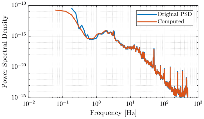

Comparison of the PSD of the original signal and the PSD of the obtained signal (png, pdf)

TODO Compute the Noise level and Signal level from PSD

<<sec:compute_psd_levels>>

Introduction   ignore

Computation

• Add table to compare the methods
• Add some explanations

  N = 10000;
  dt = 0.001;

  t = dt*(0:1:N-1)';

Parameters of the signal

  asig = 0.8; % Amplitude of the signal [V]
  fsig = 100; % Frequency of the signal [Hz]

  anoi = 1e-3; % RMS value of the noise

  x = anoi*randn(N, 1) + asig*sin((2*pi*fsig)*t);

  figure;
  plot(t, x);

Compute the PSD of the signal.

  nx = length(x);
  na = 8;
  win = blackmanharris(floor(nx/na));

  [pxx, f] = pwelch(x, win, 0, [], 1/dt);

Normalization of the PSD.

  CG = sum(win)/(nx/na);
  NG = sum(win.^2)/(nx/na);
  fbin = f(2) - f(1);

  pxx_norm = pxx*(NG*fbin/(CG)^2);

  isig = round(fsig/fbin)+1;

Estimate the Signal magnitude.

  srmt = asig/sqrt(2) % Theoretical value of signal magnitude
  srms = sqrt(sum(pxx(isig-5:isig+5)*fbin)) % Signal spectrum integrated
  srmsp = sqrt(pxx(isig) * NG*fbin/CG^2) % Maximum read off spectrum

Estimate the noise floor.

  nth = anoi/sqrt(max(f)) % Theoretical value [V/sqrt(Hz)]

  inmax = isig-20;
  nsum = sqrt(sum(pxx(1:inmax)*fbin)) / sqrt(f(inmax)) % Signal spectrum integrated

  navg = sqrt(mean(pxx(1:inmax))) % pwelch output averaged

  figure;
  hold on;
  plot(f, pxx)
  plot(f, pxx_norm)
  hold off;
  xlabel('Frequency [Hz]');
  ylabel('Power Spectral Density');
  set(gca, 'xscale', 'log');
  set(gca, 'yscale', 'log');

Bibliography   ignore

bibliographystyle:unsrt bibliography:ref.bib