phd-thesis/example-phd.org

Glossary and Acronyms - Tables

label	name	description
ka	\ensuremath{k_a}	Actuator Stiffness in
phi	\ensuremath{ɸ}	A woody bush

key	abbreviation	full form
mimo	MIMO	Multiple-Inputs Multiple-Outputs
siso	SISO	Single-Input Single-Output
nass	NASS	Nano Active Stabilization System
lti	LTI	Linear Time Invariant

Title Page

Abstract

Résumé

Acknowledgments

Table of Contents

Introduction

Test

minitoc

Abstract

Lorem Ipsum is simply dummy text of the printing and typesetting industry. Lorem Ipsum has been the industry's standard dummy text ever since the 1500s, when an unknown printer took a galley of type and scrambled it to make a type specimen book. It has survived not only five centuries, but also the leap into electronic typesetting, remaining essentially unchanged. It was popularised in the 1960s with the release of Letraset sheets containing Lorem Ipsum passages, and more recently with desktop publishing software like Aldus PageMaker including versions of Lorem Ipsum.

Test

A list:

• acronyms acrshort:nass acrshort:mimo acrshort:lti Single-Input Single-Output (SISO)
• glossary terms gls:ka, gls:phi.
• Bibliography citations: cite:&dehaeze21_activ_dampin_rotat_platf_using;&dehaeze21_mechat_approac_devel_nano_activ_stabil_system.

A definition list:

this

means that

that

means this

Some Footnote¹

Section

Sub section

This is a sub section.

Sub section

Start of the sub section

Paragraph

This is a paragraph

lksdfjasd

lksdfjasd

blabla

Source Blocks

minitoc

Figures

t = 0:0.01:5; % Time [s]
x = sin(2*pi*t); % Output Voltage [V]

figure;
plot(t, x);
xlabel('Time [s]'); ylabel('Voltage [V]');

Matlab Figure

Table Result

x = 1:10;
y = x.^2;

$x$	$y = x^2$
1	1
2	4
3	9
4	16
5	25
6	36
7	49
8	64
9	81
10	100

Table caption

Inline Results

Results can be automatically outputed as shown below.

sqrt(2)

1.4142

y

y =
     1     4     9    16    25    36    49    64    81   100

Caption and Reference

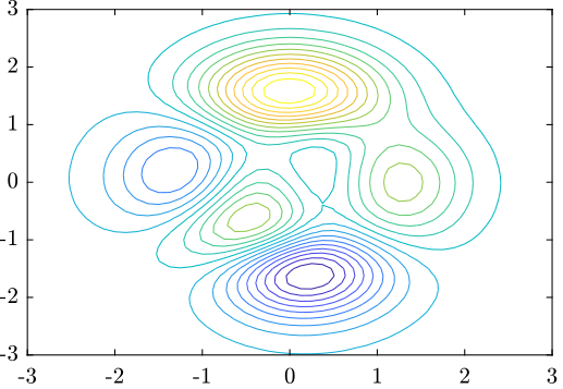
Captions can be added to code blocks. Moreover, we can link to specific bode blocks (Listing lst:matlab_figure or lst:matlab_svd).

figure;
[X,Y,Z] = peaks;
contour(X,Y,Z,20)

Code to produce a nice contour plot

Obtained Contour Plot

A = [1 2; 3 4; 5 6; 7 8]
[U,S,V] = svd(A)

A = [1 2; 3 4; 5 6; 7 8]
A =
     1     2
     3     4
     5     6
     7     8
[U,S,V] = svd(A)
U =
        -0.152483233310201         -0.82264747222566        -0.394501022283829        -0.379959133877596
        -0.349918371807964         -0.42137528768458         0.242796545704357         0.800655879510063
        -0.547353510305727       -0.0201031031435029         0.697909975442776        -0.461434357387336
         -0.74478864880349         0.381169081397575        -0.546205498863303        0.0407376117548695
S =
          14.2690954992615                         0
                         0         0.626828232417541
                         0                         0
                         0                         0
V =
        -0.641423027995072         0.767187395072177
        -0.767187395072177        -0.641423027995072

Code to compute the Singular Value Decomposition

Source Blocks with Line Numbers

Citation cite:&taghirad13_paral;&dehaeze21_activ_dampin_rotat_platf_using

The Listing lst:matlab_line_numbers has line numbers as the -n option was used.

Specific lines of codes can be referenced. For instance, the code used to specify the wanted the vertical label is on line /tdehaeze/phd-thesis/src/commit/893fabe70bfca627ed0d928d03d9cb04c4a768c0/(test).

figure;
plot(t, x)
xlabel('Time [s]');
ylabel('Output [V]'); (ref:test)

Specify Labels

Numbering can be continued by using +n option as shown below.

figure;
plot(t, u)
xlabel('Time [s]');
ylabel('Input [V]');

Images

minitoc

Normal Image

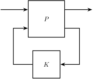
Figure fig:general_control_names shows the results of the Tikz code of listing lst:tikz_test.

  \begin{tikzpicture}

    % Blocs
    \node[block={2.0cm}{2.0cm}] (P) {$P$};
    \node[block={1.5cm}{1.5cm}, below=0.7 of P] (K) {$K$};

    % Input and outputs coordinates
    \coordinate[] (inputw)  at ($(P.south west)!0.75!(P.north west)$);
    \coordinate[] (inputu)  at ($(P.south west)!0.25!(P.north west)$);
    \coordinate[] (outputz) at ($(P.south east)!0.75!(P.north east)$);
    \coordinate[] (outputv) at ($(P.south east)!0.25!(P.north east)$);

    % Connections and labels
    \draw[<-] (inputw) -- ++(-1.5, 0);
    \draw[<-] (inputu) -- ++(-0.8, 0) |- (K.west);

    \draw[->] (outputz) -- ++(1.5, 0);
    \draw[->] (outputv) -- ++(0.8, 0) |- (K.east);
  \end{tikzpicture}

Tikz code that is used to generate Figure fig:general_control_names

General Control Configuration

Sub Images

Link to subfigure fig:general_control_names_1.

file:figs/general_control_names.png	file:figs/general_control_names.png
<<fig:general_control_names_1>> sub figure caption	<<fig:general_control_names_2>> sub figure caption

Tables

minitoc

Table tab:table_with_equations shows a table with some mathematics inside.

$N$	$N^2$	$N^3$	$N^4$	$\sqrt n$	$\sqrt[4]N$
1	1	1	1	1	1
2	4	8	16	1.4142136	1.1892071
3	9	27	81	1.7320508	1.3160740

A Simple table with included math

	1	2	3	4	5
1	1	2	3	4	5
2	2	4	6	8	10
3	3	6	9	12	15
4	4	8	12	16	20
5	5	10	15	20	25

Table without Head

	Classical Control	Modern Control
Date	1930-	1960-
Tools	Transfer Functions	State Space formulation
	Nyquist Plots	Riccati Equations
	Bode Plots
	Phase and Gain margins
Control Architectures	Proportional, Integral, Derivative	Full State Feedback
	Leads, Lags	LQR, LQG
		Kalman Filters
Advantages	Study Stability	Automatic Synthesis
	Simple	MIMO
	Natural	Optimization Problem
Disadvantages	Manual Method	No Guaranteed Robustness
	Only SISO	Difficult Rejection of Perturbations

Table with multiples groups

Appendix

Mathematical formulas

Comments on something

Bibliography

List of Publications

Glossary

Footnotes

¹this is a footnote with citation cite:&dehaeze21_mechat_approac_devel_nano_activ_stabil_system.

---