phd-test-bench-struts/test-bench-struts.org

Test Bench - Nano-Hexapod Struts

• Introduction
• Mounting Procedure
  • Introduction
  • Mounting Bench
  • Mounting Procedure
• Measurement of flexible modes
  • Introduction
  • Measurement Setup
  • Measured results
  • Conclusion
• Dynamical measurements
  • Introduction
  • Effect of the Encoder on the measured dynamics
  • Comparison of the encoder and interferometer
  • Comparison of all the Struts
  • Conclusion
• Simscape Model
  • Introduction
  • Model dynamics
  • Effect of strut misalignment
  • Measured strut misalignment
  • Proper struts alignment
  • Effect of the flexible joint
  • Conclusion
• Conclusion
• Bibliography
• Footnotes

---

This report is also available as a pdf.

---

Introduction   ignore

In this document, a test-bench is used to characterize the struts of the nano-hexapod.

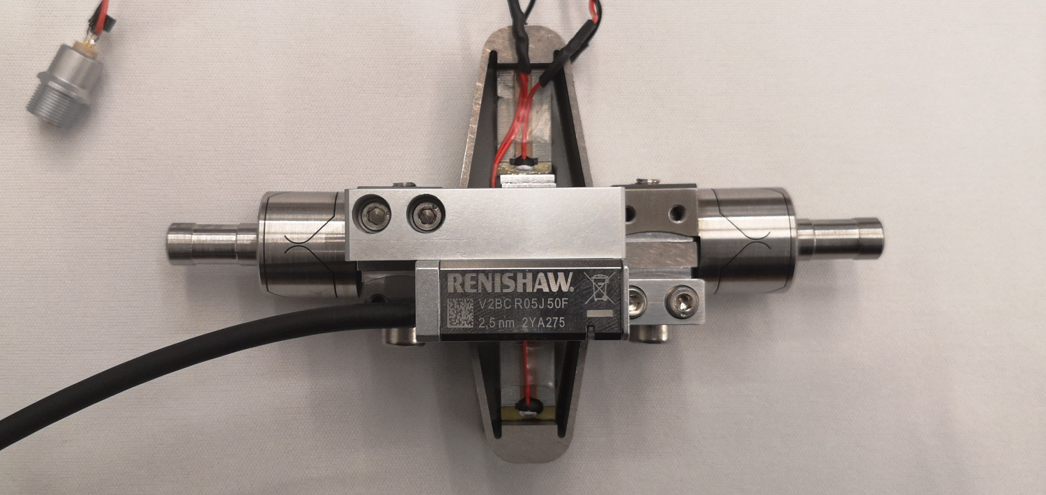
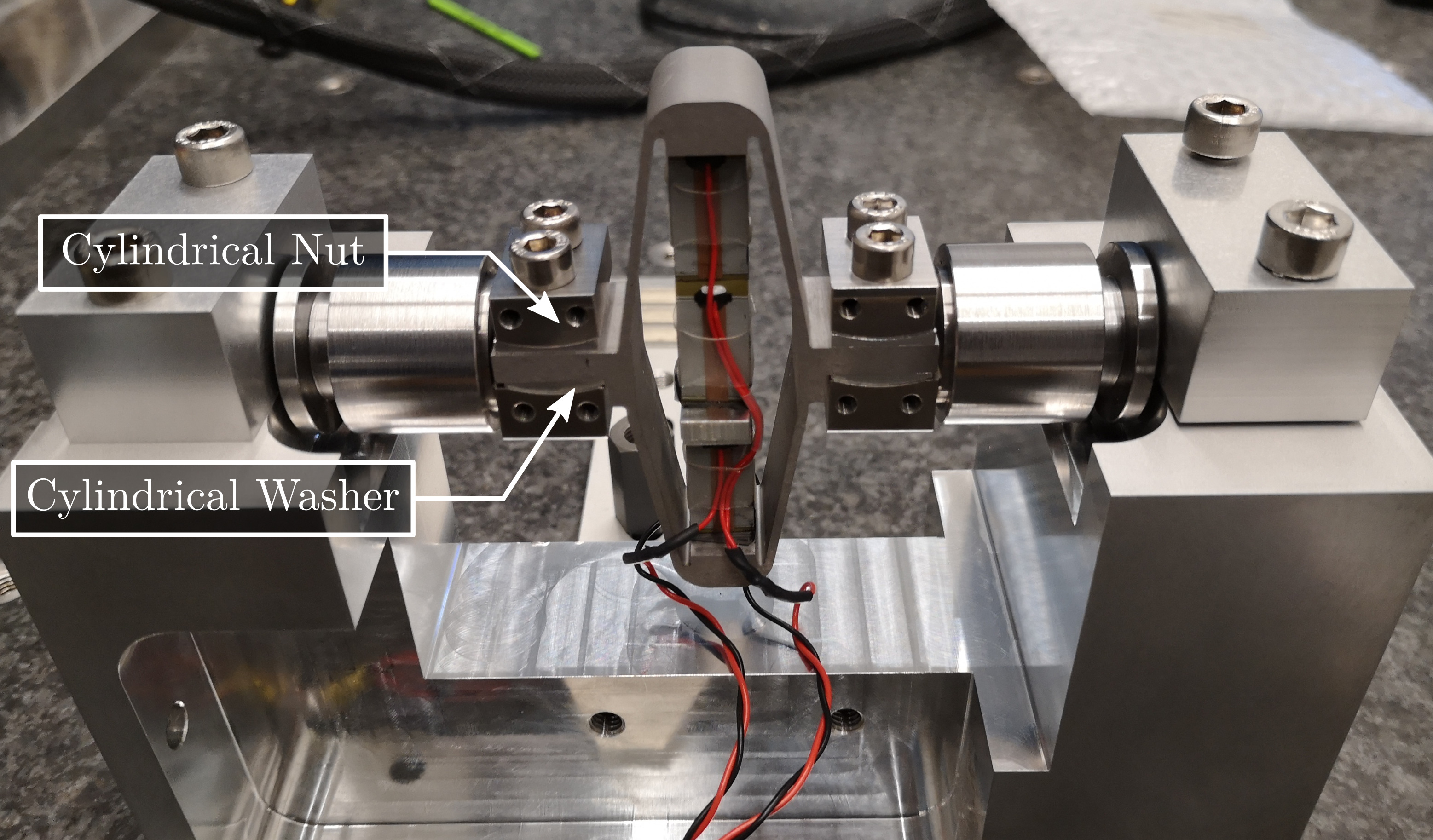
Each strut includes (Figure ref:fig:test_struts_picture_strut):

• 2 flexible joints at each ends. These flexible joints have been characterized in a separate test bench (see …).
• 1 Amplified Piezoelectric Actuator (APA300ML) (described in Section …). Two stacks are used as an actuator and one stack as a (force) sensor.
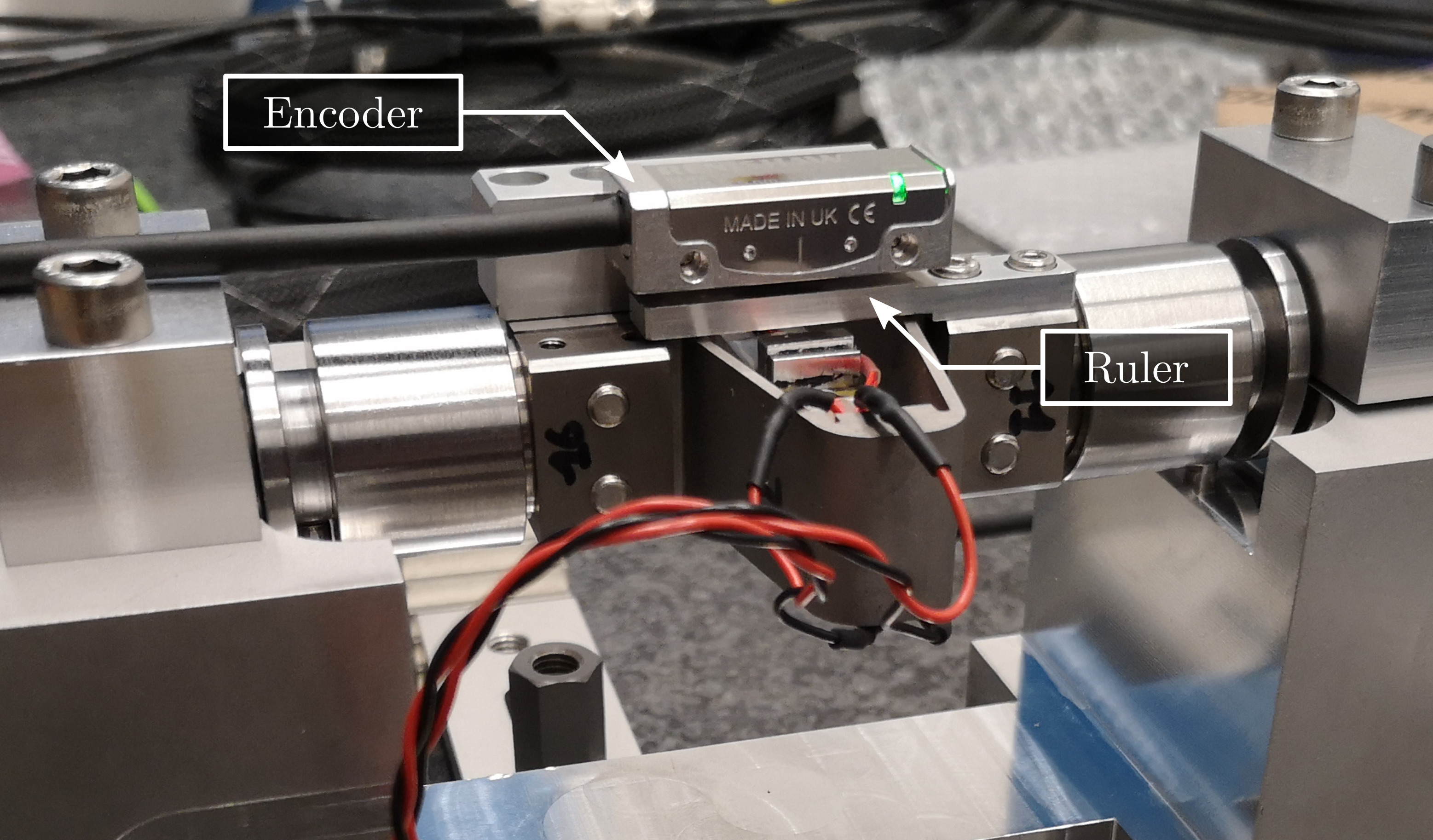
• 1 encoder (Renishaw Vionic) that has been characterized in a separate test bench (see …).

Then the struts are mounted (procedure described in Section ref:sec:test_struts_mounting), and are fixed to the same measurement bench. The goals are to:

• Section ref:sec:test_struts_dynamical_meas: Identify the dynamics from the generated DAC voltage to:

  • the sensors stack generated voltage
  • the measured displacement by the encoder
  • the measured displacement by the interferometer (representing encoders that would be fixed to the nano-hexapod's plates instead of the struts)
• Section ref:sec:test_struts_simscape: Compare the measurements with the Simscape model of the struts and tune the models

The final goal of the work presented in this document is to have an accurate Simscape model of the struts that can then be included in the Simscape model of the nano-hexapod.

Sections	Matlab File
Section ref:sec:test_struts_flexible_modes	test_struts_1_flexible_modes.m
Section ref:sec:test_struts_dynamical_meas	test_struts_2_dynamical_meas.m
Section ref:sec:test_struts_simscape	test_struts_3_simscape_model.m

Mounting Procedure

<<sec:test_struts_mounting>>

Introduction   ignore

Mounting Bench

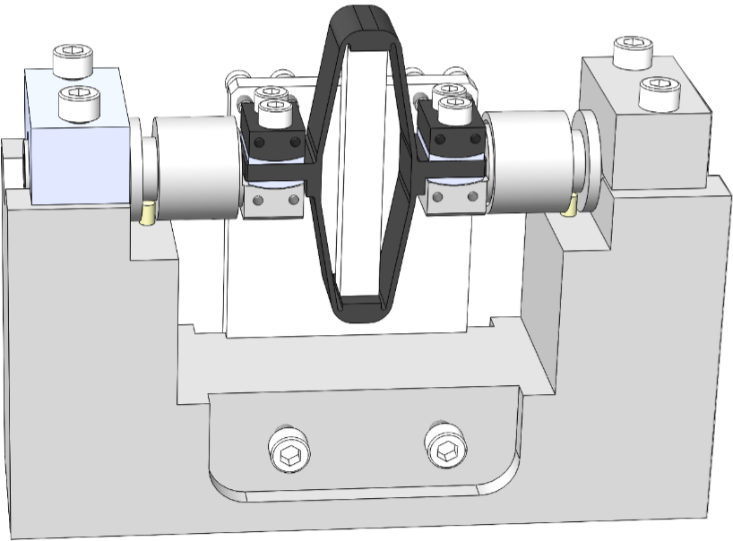
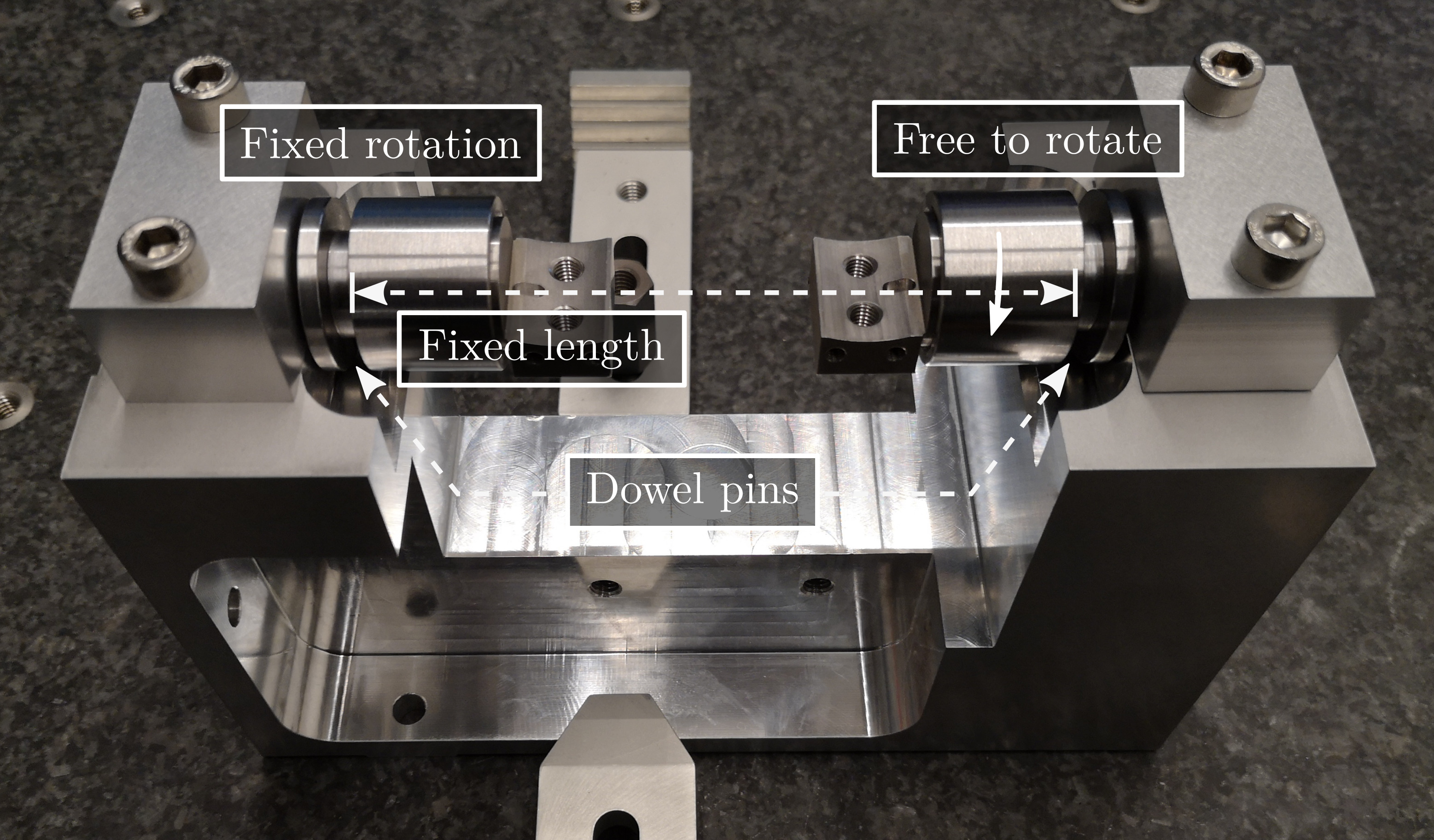
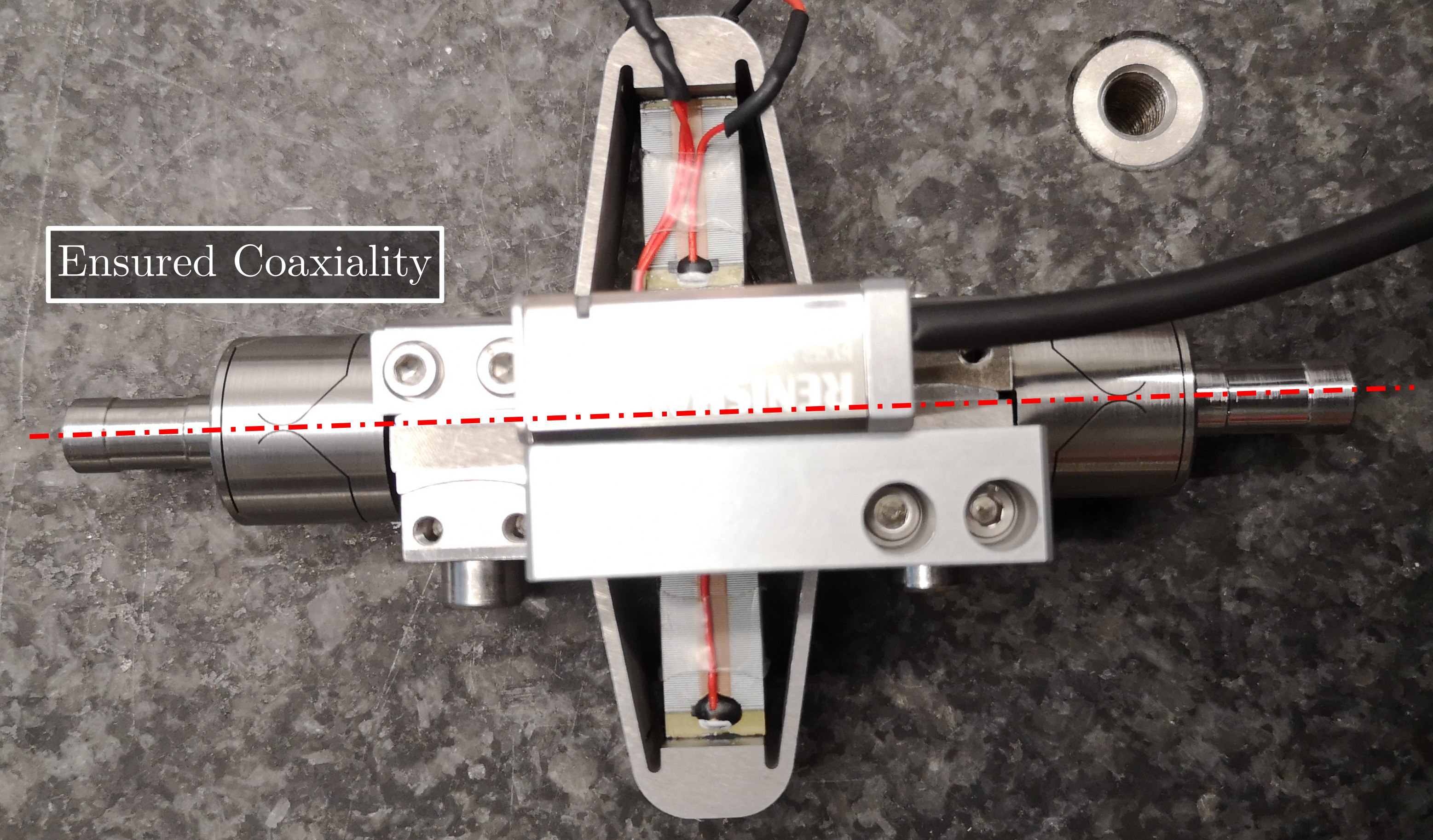
A mounting bench is used to greatly simply the mounting of the struts as well as ensuring the correct strut length and coaxiality of the flexible joint's interfaces. This is very important in order to not loose any stroke when the struts will be mounted on the nano-hexapod.

A CAD view of the mounting bench is shown in Figure ref:fig:test_struts_mounting_bench_first_concept.

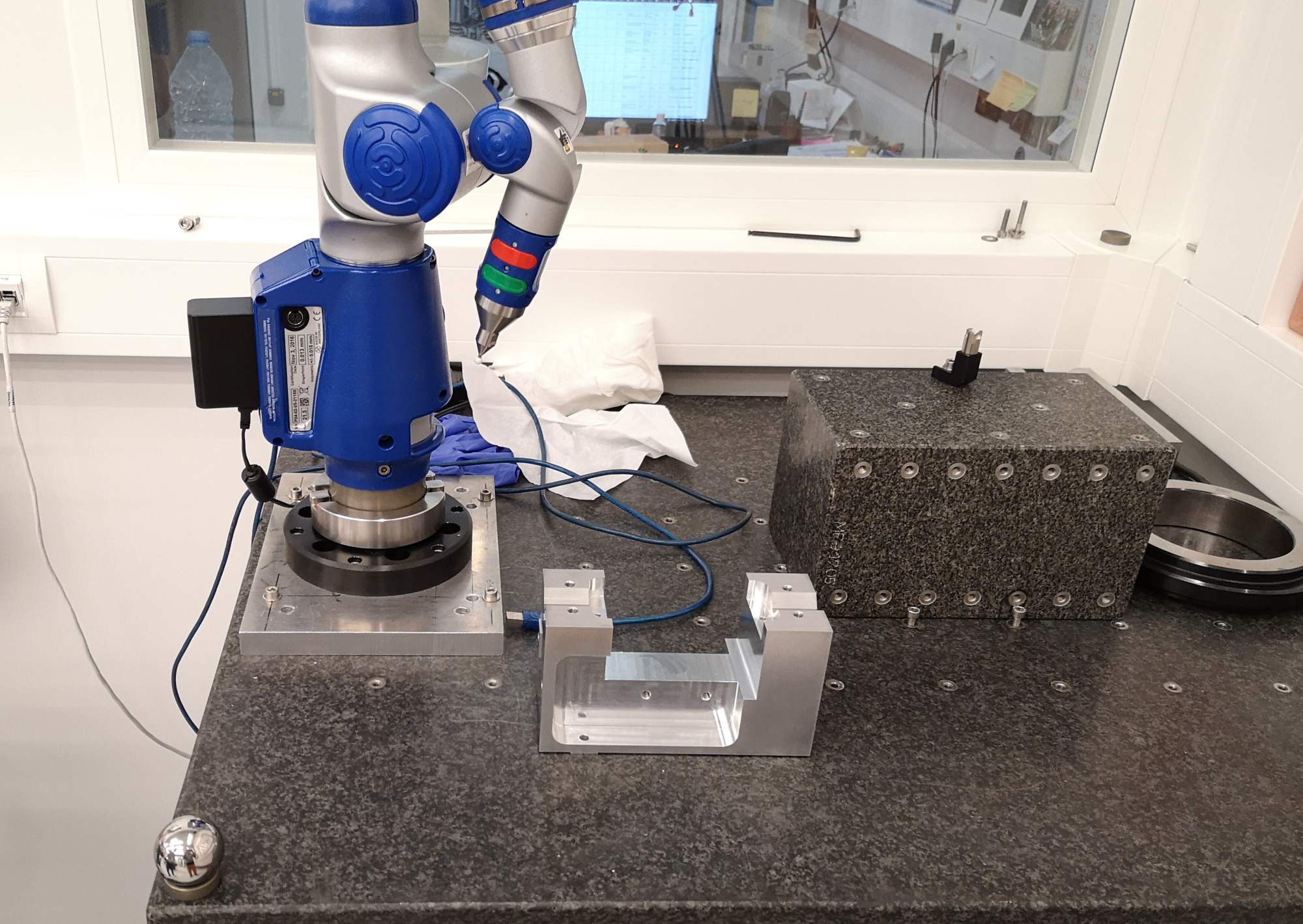
Faro arm¹

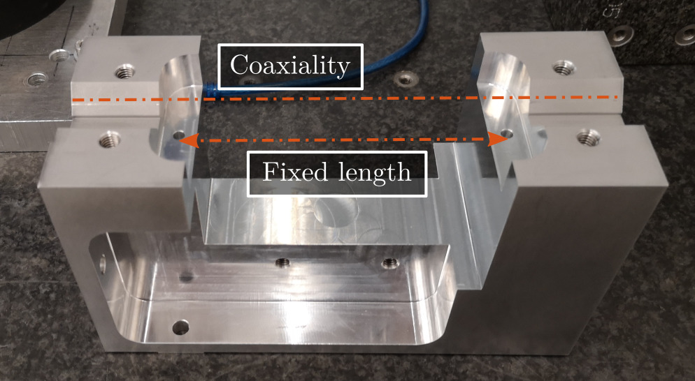
The main part of the bench is here to ensure both the correct strut length and strut coaxiality as shown in Figure ref:fig:test_struts_mounting_step_0.

The tight tolerances of this element has been verified as shown in Figure ref:fig:test_struts_check_dimensions_bench and were found to comply with the requirements.

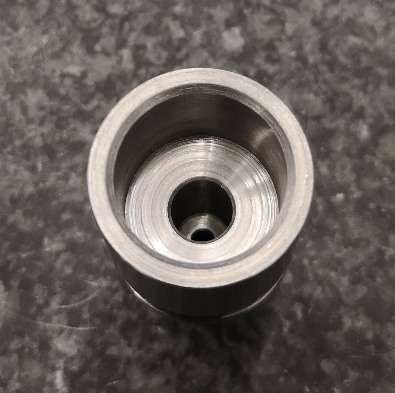
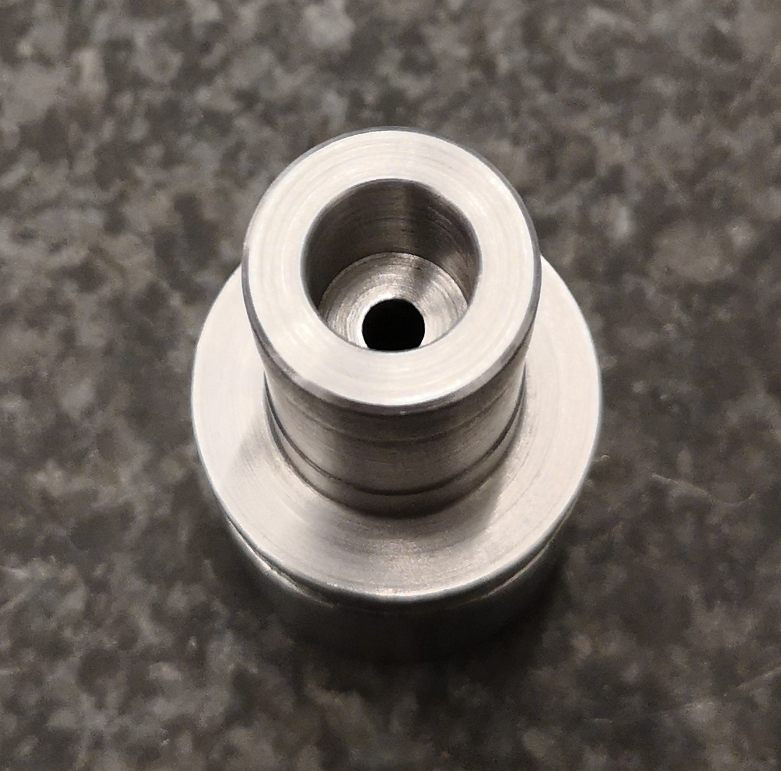
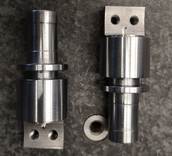
The flexible joints are rigidly fixed to cylindrical tools shown in Figures ref:fig:test_struts_cylindrical_mounting_part_top and ref:fig:test_struts_cylindrical_mounting_part_bot which are then mounted on the mounting tool shown in Figure ref:fig:test_struts_mounting_step_0. This cylindrical tool is here to protect the flexible joints when tightening the screws and therefore applying large torque.

Mounting Procedure

• Better explain the mounting procedure
• Speak about the "locating" pins that are used to aligned the APA with the two flexible joints

The mounting procedure is as follows:

1. Screw flexible joints inside the cylindrical interface element shown in Figure ref:fig:test_struts_cylindrical_mounting
2. Fix the two interface elements. One of the two should be clamped, the other one should have its axial rotation free. Visually align the clamped one horizontally. (Figure ref:fig:test_struts_mounting_step_1)
3. Put cylindrical washers, APA and interface pieces on top of the flexible joints (Figure ref:fig:test_struts_mounting_step_2)
4. Put the 4 screws just in contact such that everything is correctly positioned and such that the "free" flexible joint is correctly oriented
5. Put the 8 lateral screws in contact
6. Tighten the 4 screws to fix the APA on the two flexible joints (using a torque screwdriver)
7. Remove the 4 laterals screws
8. (optional) Put the APA horizontally and fix the encoder and align it to maximize the contrast (Figure ref:fig:test_struts_mounting_step_3)
9. Disassemble to have an properly mounted strut (Figure ref:fig:test_struts_mounting_step_4) for which the coaxiality between the two flexible joint's interfaces is good

\bigskip

Measurement of flexible modes

<<sec:test_struts_flexible_modes>>

Introduction

From a Finite Element Model of the struts, it have been found that three main resonances are foreseen to be problematic for the control of the APA300ML (Figure ref:fig:test_struts_mode_shapes): an "X-bending" mode at 189Hz, a "Y-bending" mode at 285Hz and a "Z-torsion" mode at 400Hz.

Measurement Setup

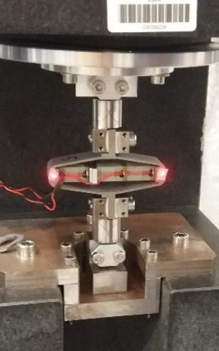
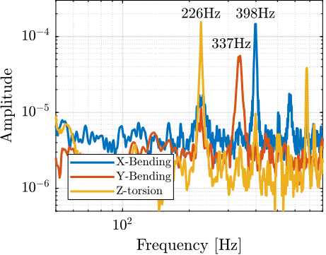
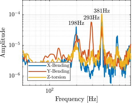
A Laser vibrometer is measuring the difference of motion between two beam path (red points in Figure ref:fig:test_struts_meas_modes). The strut is excited with an instrumented hammer and the transfer function from the hammer to the measured rotation is computed.

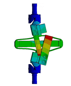
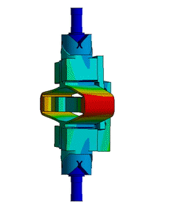
The "X-bending" mode is measured as shown in Figure ref:fig:test_struts_meas_x_bending. The "Y-bending" mode is measured as shown in Figure ref:fig:test_struts_meas_y_bending. Finally, the "Z-torsion" is measured as shown in Figure ref:fig:test_struts_meas_z_torsion.

This is done with and without the encoder fixed to the strut.

Measured results

The obtained frequency response functions are shown in Figure ref:fig:test_struts_spur_res_frf.

Conclusion   ignore

Table ref:tab:test_struts_spur_mode_freqs summarizes the measured resonance frequencies as well as the computed ones using the Finite Element Model. It is shown that:

• the resonance frequencies of the 3 modes are only slightly increasing when the encoder is removed
• the computed resonance frequencies from the FEM are very close to the measured one when the encoder is fixed to the strut

Mode	Struts (FEM)	Struts (exp)	Plates (exp)
X-Bending	189Hz	198Hz	226Hz
Y-Bending	285Hz	293Hz	337Hz
Z-Torsion	400Hz	381Hz	398Hz

Dynamical measurements

<<sec:test_struts_dynamical_meas>>

Introduction   ignore

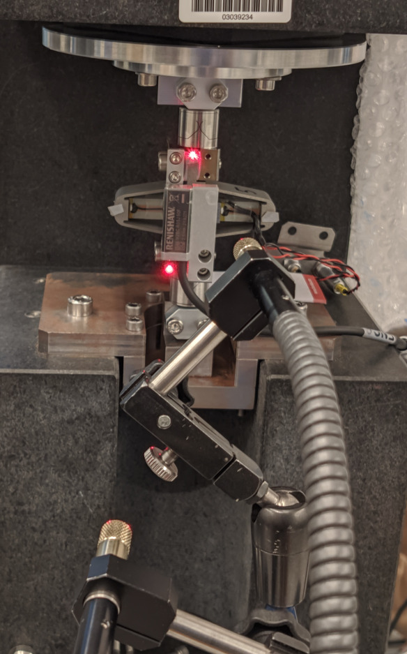
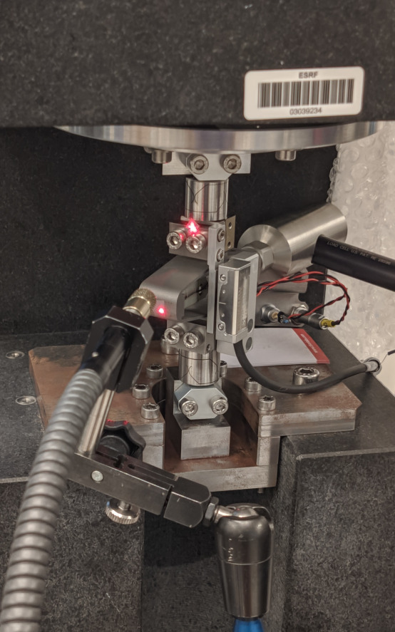
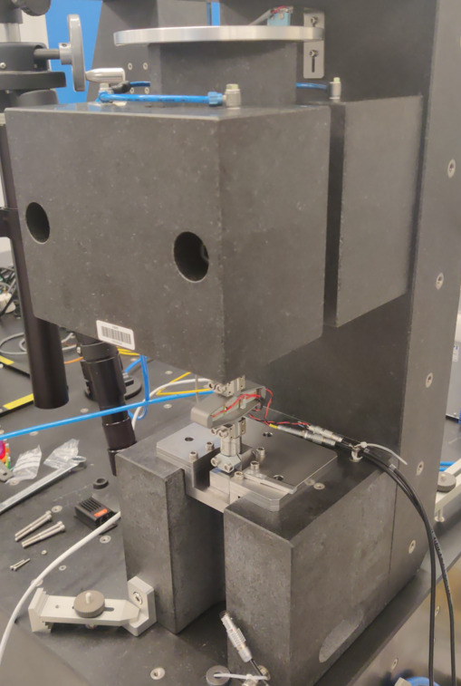
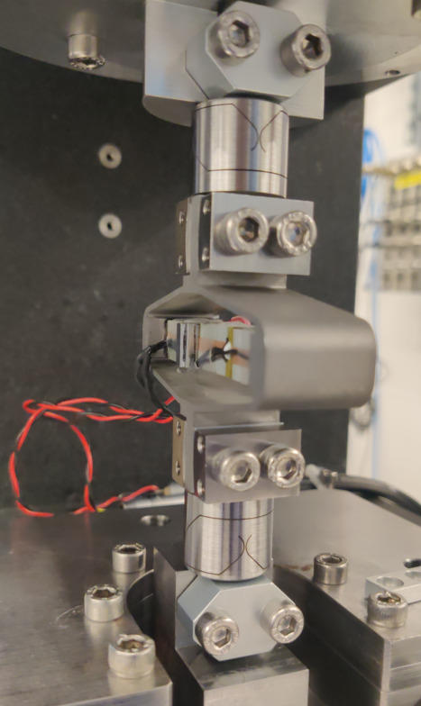
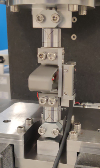
The bench is shown in Figure ref:fig:test_struts_bench_leg_overview. Measurements are performed either when no encoder is fixed to the strut (Figure ref:fig:test_struts_bench_leg_front) or when one encoder is fixed to the strut (Figure ref:fig:test_struts_bench_leg_coder).

First, the effect of the encoder on the measured dynamics is studied in Section ref:ssec:test_struts_effect_encoder. Then, the dynamics seen by the encoder and by the interferometers are compared in Section ref:ssec:test_struts_comp_enc_int. Finally, all the measured struts are compared in terms of dynamics in Section ref:ssec:test_struts_comp_all_struts.

Effect of the Encoder on the measured dynamics

<<ssec:test_struts_effect_encoder>>

%% Parameters for Frequency Analysis
Ts = 1e-4; % Sampling Time [s]
Nfft = floor(1/Ts); % Number of points for the FFT computation
win = hanning(Nfft); % Hanning window
Noverlap = floor(Nfft/2); % Overlap between frequency analysis

%% Measure FRF for Strut 1 - No encoder
% Load Data
leg_sweep    = load('frf_data_leg_1_sweep.mat', 'u', 'Vs', 'de', 'da');
leg_noise_hf = load('frf_data_leg_1_noise_hf.mat', 'u', 'Vs', 'de', 'da');

% We get the frequency vector that will be the same for all the frequency domain analysis.
[~, f] = tfestimate(leg_sweep.u, leg_sweep.de, win, Noverlap, Nfft, 1/Ts);
i_lf = f <= 350; % Indices used for the low frequency
i_hf = f >  350; % Indices used for the high frequency

% Compute FRF function from u to da (interferometer)
[frf_sweep, ~]    = tfestimate(leg_sweep.u,    leg_sweep.da,    win, Noverlap, Nfft, 1/Ts);
[frf_noise_hf, ~] = tfestimate(leg_noise_hf.u, leg_noise_hf.da, win, Noverlap, Nfft, 1/Ts);
int_frf = [frf_sweep(i_lf); frf_noise_hf(i_hf)]; % Combine the FRF

% Compute FRF function from u to Vs (force sensor)
[frf_sweep,    ~] = tfestimate(leg_sweep.u,    leg_sweep.Vs,    win, Noverlap, Nfft, 1/Ts);
[frf_noise_hf, ~] = tfestimate(leg_noise_hf.u, leg_noise_hf.Vs, win, Noverlap, Nfft, 1/Ts);
iff_frf = [frf_sweep(i_lf); frf_noise_hf(i_hf)]; % Combine the FRF

%% Measure FRF for Strut 1 - With encoder
% Load Data
leg_enc_sweep    = load('frf_data_leg_coder_1_noise.mat',    'u', 'Vs', 'de', 'da');
leg_enc_noise_hf = load('frf_data_leg_coder_1_noise_hf.mat', 'u', 'Vs', 'de', 'da');

% Compute FRF function from u to da (interferometer)
[frf_sweep, ~]    = tfestimate(leg_enc_sweep.u,    leg_enc_sweep.da,    win, Noverlap, Nfft, 1/Ts);
[frf_noise_hf, ~] = tfestimate(leg_enc_noise_hf.u, leg_enc_noise_hf.da, win, Noverlap, Nfft, 1/Ts);
int_with_enc_frf = [frf_sweep(i_lf); frf_noise_hf(i_hf)]; % Combine the FRF

% Compute FRF function from u to Vs (force sensor)
[frf_sweep, ~]    = tfestimate(leg_enc_sweep.u,    leg_enc_sweep.Vs,    win, Noverlap, Nfft, 1/Ts);
[frf_noise_hf, ~] = tfestimate(leg_enc_noise_hf.u, leg_enc_noise_hf.Vs, win, Noverlap, Nfft, 1/Ts);
iff_with_enc_frf = [frf_sweep(i_lf); frf_noise_hf(i_hf)]; % Combine the FRF

% Compute FRF function from u to de (encoder)
[frf_sweep, ~]    = tfestimate(leg_enc_sweep.u,    leg_enc_sweep.de,    win, Noverlap, Nfft, 1/Ts);
[frf_noise_hf, ~] = tfestimate(leg_enc_noise_hf.u, leg_enc_noise_hf.de, win, Noverlap, Nfft, 1/Ts);
enc_frf = [frf_sweep(i_lf); frf_noise_hf(i_hf)]; % Combine the FRF

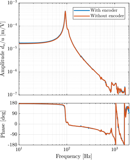
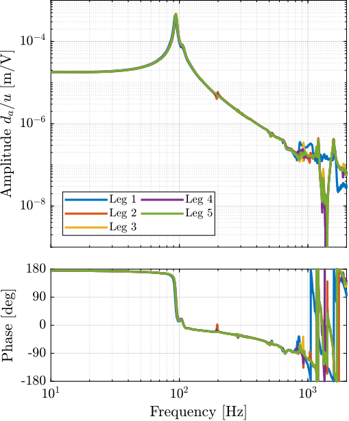
Figure ref:fig:test_struts_effect_encoder_int Same goes for the transfer function from excitation voltage $u$ to the axial motion of the strut $d_a$ as measured by the interferometer ().

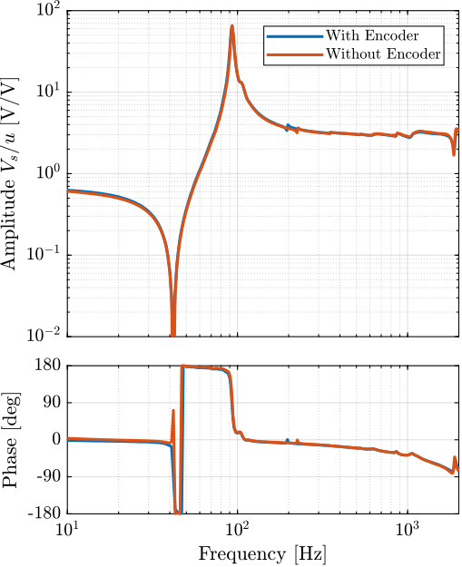
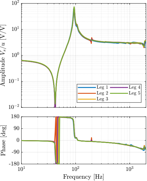
The transfer function from the excitation voltage $u$ to the generated voltage $V_s$ by the sensor stack is not influence by the fixation of the encoder (Figure ref:fig:test_struts_effect_encoder_iff). This means that the IFF control strategy should be as effective whether or not the encoders are fixed to the struts.

Comparison of the encoder and interferometer

<<ssec:test_struts_comp_enc_int>>

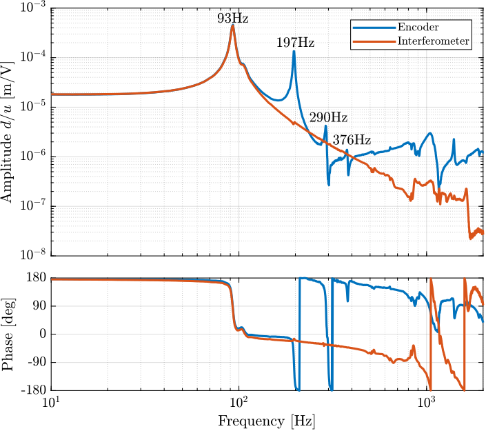
The dynamics as measured by the encoder and by the interferometers are compared in Figure ref:fig:test_struts_comp_enc_int.

The dynamics from the excitation voltage $u$ to the measured displacement by the encoder $d_e$ presents much more complicated behavior than the transfer function to the displacement as measured by the Interferometer (compared in Figure ref:fig:test_struts_comp_enc_int). It will be further investigated why the two dynamics as so different and what are causing all these resonances.

As shown in Figure ref:fig:test_struts_comp_enc_int, we can clearly see three spurious resonances at 197Hz, 290Hz and 376Hz. These resonances correspond to parasitic resonances of the strut itself that was estimated using a finite element model of the strut (Figure ref:fig:test_struts_mode_shapes):

• Mode in X-bending at 189Hz
• Mode in Y-bending at 285Hz
• Mode in Z-torsion at 400Hz

The good news is that these resonances are not seen on the interferometer (they are therefore not impacting the axial motion of the strut). But these resonances are making the use of encoder fixed to the strut difficult.

Comparison of the transfer functions from excitation voltage $u$ to either the encoder $d_e$ or the interferometer $d_a$

Comparison of all the Struts

<<ssec:test_struts_comp_all_struts>>

%% Numbers of the measured legs
strut_nums = [1 2 3 4 5];

%% Load the measurement data
% First identification (low frequency noise)
leg_noise = {};
for i = 1:length(strut_nums)
    leg_noise(i) = {load(sprintf('frf_data_leg_coder_%i_noise.mat', strut_nums(i)), 'u', 'Vs', 'de', 'da')};
end

% Second identification (high frequency noise)
leg_noise_hf = {};
for i = 1:length(strut_nums)
    leg_noise_hf(i) = {load(sprintf('frf_data_leg_coder_%i_noise_hf.mat', strut_nums(i)), 'u', 'Vs', 'de', 'da')};
end

%% Compute FRF - From u to de (encoder)
enc_frf = zeros(length(f), length(strut_nums));

for i = 1:length(strut_nums)
    [frf_lf, ~] = tfestimate(leg_noise{i}.u,    detrend(leg_noise{i}.de, 0),    win, Noverlap, Nfft, 1/Ts);
    [frf_hf, ~] = tfestimate(leg_noise_hf{i}.u, detrend(leg_noise_hf{i}.de, 0), win, Noverlap, Nfft, 1/Ts);
    enc_frf(:, i) = [frf_lf(i_lf); frf_hf(i_hf)];
end

%% Compute FRF - From u to da (interferometer)
int_frf = zeros(length(f), length(strut_nums));
for i = 1:length(strut_nums)
    [frf_lf, ~] = tfestimate(leg_noise{i}.u,    leg_noise{i}.da,    win, Noverlap, Nfft, 1/Ts);
    [frf_hf, ~] = tfestimate(leg_noise_hf{i}.u, leg_noise_hf{i}.da, win, Noverlap, Nfft, 1/Ts);
    int_frf(:, i) = [frf_lf(i_lf); frf_hf(i_hf)];
end

%% Compute FRF - From u to Vs (force sensor)
iff_frf = zeros(length(f), length(strut_nums));
for i = 1:length(strut_nums)
    [frf_lf, ~] = tfestimate(leg_noise{i}.u,    leg_noise{i}.Vs,    win, Noverlap, Nfft, 1/Ts);
    [frf_hf, ~] = tfestimate(leg_noise_hf{i}.u, leg_noise_hf{i}.Vs, win, Noverlap, Nfft, 1/Ts);
    iff_frf(:, i) = [frf_lf(i_lf); frf_hf(i_hf)];
end

Then, the transfer function from the DAC output voltage $u$ to the measured displacement by the Attocube is computed for all the struts and shown in Figure ref:fig:test_struts_comp_interf_plants. All the struts are giving very similar FRF.

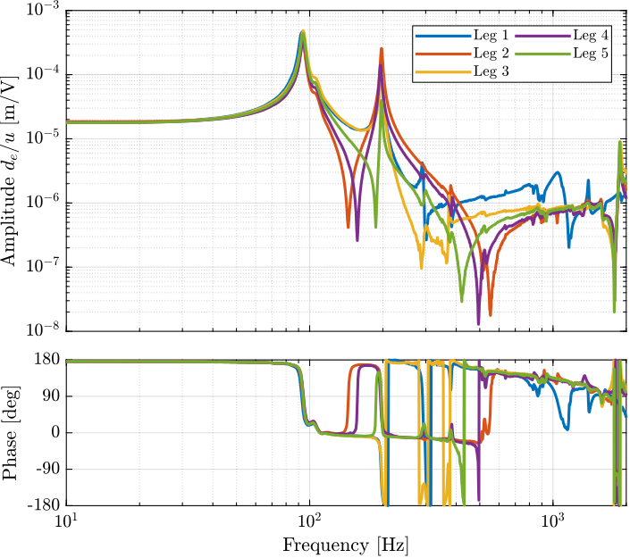
There is a very large variability of the dynamics as measured by the encoder as shown in Figure ref:fig:test_struts_comp_enc_plants. Even-though the same peaks are seen for all of the struts (95Hz, 200Hz, 300Hz, 400Hz), the amplitude of the peaks are not the same. Moreover, the location or even the presence of complex conjugate zeros is changing from one strut to the other.

All of this will be studied in Section ref:sec:test_struts_simscape using the Simscape model.

Estimated frequency response functions from $u$ to the encoder $d_e$ for all the mounted struts

Conclusion   ignore

All the struts are giving very consistent behavior from the excitation voltage $u$ to the force sensor generated voltage $V_s$ and to the interferometer measured displacement $d_a$. However, the dynamics from $u$ to the encoder measurement $d_e$ is much more complex and variable from one strut to the other most likely due to poor alignment of the APA with respect to the flexible joints.

%% Save the estimated FRF for further analysis
save('./mat/meas_struts_frf.mat', 'f', 'enc_frf', 'int_frf', 'iff_frf', 'strut_nums');

Simscape Model

<<sec:test_struts_simscape>>

Introduction   ignore

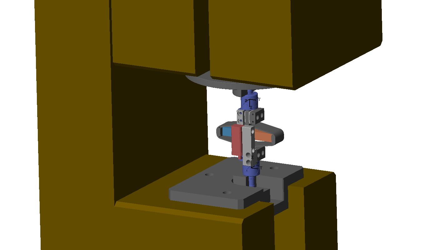
However, now the full strut is put instead of only the APA (see Figure ref:fig:test_struts_simscape_model).

This Simscape model is used to:

• compare the measured FRF with the modelled FRF
• help the correct understanding/interpretation of the results
• tune the model of the struts (APA, flexible joints, encoder)

This study is structured as follow:

• Section ref:ssec:test_struts_comp_model: the measured FRF are compared with the Simscape model.
• Section ref:ssec:test_struts_effect_misalignment: the flexible APA model is used, and the effect of a misalignment of the APA and flexible joints is studied. It is found that the misalignment has a large impact on the dynamics from $u$ to $d_e$.
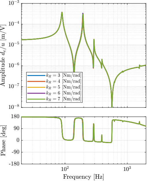
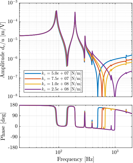
• Section ref:ssec:test_struts_effect_joint_stiffness: the effect of the flexible joint's stiffness on the dynamics is studied. It is found that the axial stiffness of the joints has a large impact on the location of the zeros on the transfer function from $V_s$ to $d_e$.

Model dynamics

<<ssec:test_struts_comp_model>>

%% Load measured FRF for comparison
load('meas_struts_frf.mat', 'f', 'enc_frf', 'int_frf', 'iff_frf', 'strut_nums');

%% Initialize strut with 2DoF model for the APA300ML and identify the dynamics
n_hexapod = struct();
n_hexapod.flex_bot = initializeBotFlexibleJoint('type', '4dof');
n_hexapod.flex_top = initializeTopFlexibleJoint('type', '4dof');
n_hexapod.actuator = initializeAPA('type', '2dof');

c_granite = 0; % Do not take into account damping added by the air bearing

% Run the linearization
Gs_2dof = exp(-s*1e-4)*linearize(mdl, io, 0.0, opts);
Gs_2dof.InputName  = {'u'};
Gs_2dof.OutputName = {'Vs', 'de', 'da'};

%% Initialize strut with "flexible" model for the APA300ML and identify the dynamics
n_hexapod = struct();
n_hexapod.flex_bot = initializeBotFlexibleJoint('type', '4dof');
n_hexapod.flex_top = initializeTopFlexibleJoint('type', '4dof');
n_hexapod.actuator = initializeAPA('type', 'flexible');

c_granite = 100; % Do not take into account damping added by the air bearing

% Run the linearization
Gs_flex = exp(-s*1e-4)*linearize(mdl, io, 0.0, opts);
Gs_flex.InputName  = {'u'};
Gs_flex.OutputName = {'Vs', 'de', 'da'};

Two models of the APA300ML are used here for comparison:

• a simple two degrees of freedom model
• a model using a super element extracted from a finite element model

These two models of the APA300ML were tuned to best match measured frequency response functions of the APA alone. The flexible joints are here modelled with the 4DoF model (axial stiffness, two bending stiffnesses and one torsion stiffness).

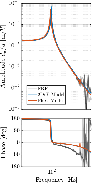
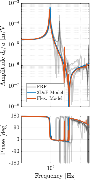
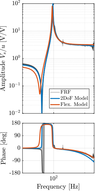
These two models are compared with the measured frequency responses in Figure ref:fig:test_struts_comp_frf_flexible_model.

The model dynamics from DAC voltage $u$ to the axial motion of the strut $d_a$ (Figure ref:fig:test_struts_comp_frf_flexible_model_int) and from DAC voltage $u$ to the force sensor voltage $V_s$ (Figure ref:fig:test_struts_comp_frf_flexible_model_iff) are well matching the experimental identification.

However, the transfer function from $u$ to encoder displacement $d_e$ are not well matching for both models. For the 2DoF model, this is normal as the resonances affecting the dynamics are not modelled at all (the APA300ML is modelled as infinitely rigid in all directions except the translation along it's actuation axis). For the flexible model, it will be shown in the next section that by adding some misalignment betwen the flexible joints and the APA300ML, this model can better represent the observed dynamics.

Effect of strut misalignment

<<ssec:test_struts_effect_misalignment>>

As was shown in Figure ref:fig:test_struts_comp_enc_plants, the identified dynamics from DAC voltage $u$ to encoder measured displacement $d_e$ are very different from one strut to the other.

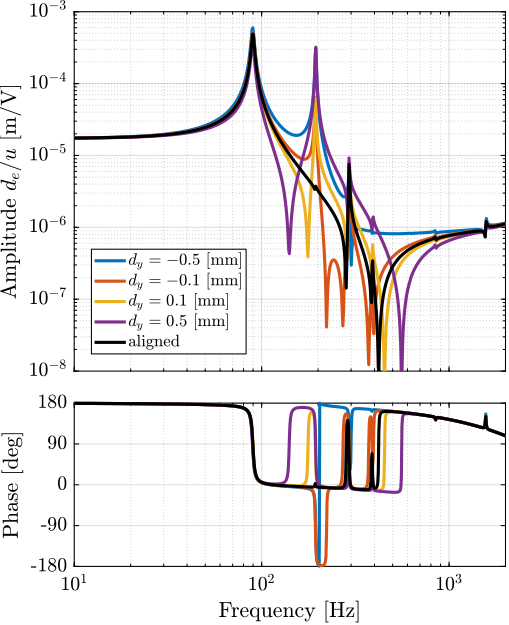
In this section, it is investigated whether poor alignment of the strut (flexible joints with respect to the APA) can explain such dynamics. For instance, consider Figure ref:fig:test_struts_misalign_schematic where there is a misalignment in the $y$ direction between the two flexible joints (well aligned thanks to the mounting procedure in Section ref:sec:test_struts_mounting) and the APA300ML. In such case, the "x-bending" mode at 200Hz (see Figure ref:fig:test_struts_meas_x_bending) can be expected to be more excited, and thus the dynamics from the actuator to the encoder should be affected at frequencies around 200Hz.

To verify this assumption, the dynamics from output DAC voltage $u$ to the measured displacement by the encoder $d_e$ is computed using the Simscape model with flexible APA for several misalignment in the $y$ direction. Obtained dynamics are shown in Figure ref:fig:test_struts_effect_misalignment_y. The alignment of the APA with the flexible joints as a huge influence on the dynamics from actuator voltage to measured displacement by the encoder. The misalignment in the $y$ direction mostly influences:

• the presence of the flexible mode at 200Hz (see mode shape in Figure ref:fig:test_struts_mode_shapes_1)

• the location of the complex conjugate zero between the first two resonances:

  • if $d_y < 0$: there is no zero between the two resonances and possibly not even between the second and third ones
  • if $d_y > 0$: there is a complex conjugate zero between the first two resonances
• the location of the high frequency complex conjugate zeros at 500Hz (secondary effect, as the axial stiffness of the joint also has large effect on the position of this zero)

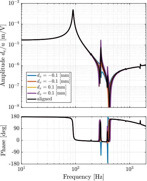
The same can be done for a misalignment in the $x$ direction. The obtained dynamics are shown in Figure ref:fig:test_struts_effect_misalignment_x where it is shown that misalignment in the $x$ direction mostly influences the presence of the flexible mode at 300Hz (see mode shape in Figure ref:fig:test_struts_mode_shapes_2).

Comparing the experimental frequency response functions for all the APA in Figure ref:fig:test_struts_comp_enc_plants with the model dynamics for several $y$ misalignments in Figure ref:fig:test_struts_effect_misalignment_y indicates a clear similarity. This similarity suggests that the identified differences in dynamics are caused by the misalignment.

%% Effect of a misalignment in Y-Direction
% Considered misalignment in the Y direction
dy_aligns = [-0.5, -0.1, 0.1, 0.5]*1e-3; % [m]

% Transfer functions from u to de for all the misalignment in y direction
Gs_dy_align = {zeros(length(dy_aligns), 1)};

for i = 1:length(dy_aligns)
    n_hexapod.actuator = initializeAPA('type', 'flexible', 'd_align_bot', [0; dy_aligns(i); 0], 'd_align_top', [0; dy_aligns(i); 0]);

    G = exp(-s*1e-4)*linearize(mdl, io, 0.0, opts);
    G.InputName  = {'u'};
    G.OutputName = {'Vs', 'de', 'da'};

    Gs_dy_align(i) = {G};
end

%% Effect of a misalignment in X-Direction
% Considered misalignment in the X direction
dx_aligns = [-0.1, -0.05, 0.05, 0.1]*1e-3; % [m]

% Transfer functions from u to de for all the misalignment in x direction
Gs_dx_align = {zeros(length(dx_aligns), 1)};

for i = 1:length(dx_aligns)
    n_hexapod.actuator = initializeAPA('type', 'flexible', 'd_align_bot', [dx_aligns(i); 0; 0], 'd_align_top', [dx_aligns(i); 0; 0]);

    G = exp(-s*1e-4)*linearize(mdl, io, 0.0, opts);
    G.InputName  = {'u'};
    G.OutputName = {'Vs', 'de', 'da'};

    Gs_dx_align(i) = {G};
end

Measured strut misalignment

<<ssec:test_struts_meas_misalignment>>

During the first mounting of the struts presented in Section ref:sec:test_struts_mounting, the positioning pins used to position the APA with respect to the flexible joints in the $y$ directions were not used (not received at the time). Therefore, large $y$ misalignments may be expected.

In order to estimate the misalignments between the two flexible joints and the APA:

• the struts are fixed horizontally to the mounting bench as shown in Figure ref:fig:test_struts_mounting_step_3 but without the encoder
• using a length gauge², the height difference from the flexible joints surface and the APA shell surface is measured both for the top and bottom joints and on both sides
• as the thickness of the flexible joint is $21\,mm$ and the thickness of the APA shell is $20\,mm$, $0.5\,mm$ of height different should be measured is the two are perfectly aligned

Large variations in the $y$ misalignment are found from one strut to the other (results are summarized in Table ref:tab:test_struts_meas_y_misalignment).

To check the validity of the measurement, it can be verified that sum of the measured thickness difference on each side is $1\,mm$ (equal to the thickness difference between the flexible joint and the APA). This thickness differences for all the struts were found to be between $0.94\,mm$ and $1.00\,mm$ which indicate low errors as compared to the misalignments found in Table ref:tab:test_struts_meas_y_misalignment.

%% Measurement of the y misalignment between the APA and the flexible joints
% Mesured struts
strut_nums = [1, 2, 3, 4, 5];

% Measured height differences in [mm]
% R ("red" side), B ("black" side)
%                R Top  B Top  R Bot  B Bot
strut_align = [[-0.40, -0.60, -0.16, -0.82]   % Strut 1
               [-0.67, -0.30, -0.34, -0.63]   % Strut 2
               [-0.07, -0.88, -0.16, -0.79]   % Strut 3
               [-0.48, -0.46,  0.07, -1.00]   % Strut 4
               [-0.33, -0.64, -0.48, -0.52]]; % Strut 5

% Verification that the thickness difference between the APA shell and the flexible joints is 1mm
thichness_diff_top = strut_align(:,1) + strut_align(:,2); % [mm]
thichness_diff_bot = strut_align(:,1) + strut_align(:,2); % [mm]

% Estimation of the dy misalignment
dy_bot = (strut_align(:,1) - strut_align(:,2))/2; % [mm]
dy_top = (strut_align(:,3) - strut_align(:,4))/2; % [mm]

Strut	Bot	Top
1	0.1	0.33
2	-0.19	0.14
3	0.41	0.32
4	-0.01	0.54
5	0.15	0.02

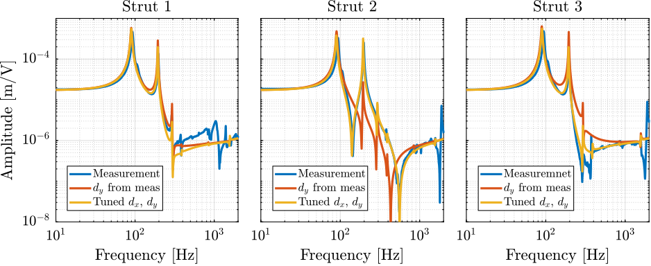
By using the measured $y$ misalignment in the Simscape model with the flexible APA model, the measured dynamics from $u$ to $d_e$ can be approached as shown in Figure ref:fig:test_struts_comp_dy_tuned_model_frf_enc. Even better match in the dynamics can be obtained by fine tuning both the $x$ and $y$ misalignments (yellow curves in Figure ref:fig:test_struts_comp_dy_tuned_model_frf_enc).

This confirms that the misalignment between the APA and the strut axis (determined by the two flexible joints) is critical and is inducing large variations in the dynamics from DAC voltage $u$ to encoder measured displacement $d_e$. If encoders are to be used when fixed on the struts, it is therefore very important to properly align the APA and the flexible joints when mounting the struts.

In the next section, the struts are re-assembled with a "positioning pin" to better align the APA with the flexible joints. With a better alignment, the amplitude of the spurious resonances are expected to decrease as was shown in Figure ref:fig:test_struts_effect_misalignment_y.

%% Idenfity the dynamics from u to de - misalignement estimated from measurement
Gs_y_align = {zeros(size(strut_align,1), 1)};

% Measured dy alignment
strut_align = 1e-3*[[-0.60, -0.82, -0.40, -0.16]
                    [-0.30, -0.63, -0.67, -0.34]
                    [-0.88, -0.79, -0.07, -0.16]
                    [-0.48,  0.07, -0.46, -1.00]
                    [-0.33, -0.48, -0.64, -0.52]
                    [-0.34, -0.42, -0.63, -0.57]];

for i = 1:size(strut_align,1)
    n_hexapod.actuator = initializeAPA('type', 'flexible', ...
                                       'd_align_bot', [0; strut_align(i, 2) - strut_align(i, 4); 0], ...
                                       'd_align_top', [0; strut_align(i, 1) - strut_align(i, 3); 0]);

    G = exp(-s*1e-4)*linearize(mdl, io, 0.0, opts);
    G.InputName  = {'u'};
    G.OutputName = {'Vs', 'de', 'da'};

    Gs_y_align(i) = {G};
end

%% Idenfity the dynamics from u to de - misalignement tuned to have the best match
d_aligns = [[-0.05,  -0.3,  0];
            [ 0,      0.5,  0];
            [-0.1,   -0.3,  0];
            [ 0,      0.3,  0];
            [-0.05,   0.05, 0]]'*1e-3;

% Idenfity the transfer function from actuator to encoder for all cases
Gs_xy_align = {zeros(size(d_aligns,2), 1)};

for i = 1:5
    n_hexapod.actuator = initializeAPA('type', 'flexible', 'd_align_top', d_aligns(:,i), 'd_align_bot', d_aligns(:,i));

    G = exp(-s*1e-4)*linearize(mdl, io, 0.0, opts);
    G.InputName  = {'u'};
    G.OutputName = {'Vs', 'de', 'da'};

    Gs_xy_align(i) = {G};
end

Comparison of the frequency response functions from DAC voltage $u$ to measured displacement $d_e$ by the encoders for three struts. In blue the measured dynamics, in red the dynamics extracted from the model with the $y$ misalignment estimated from measurements, in yellow the dynamics extracted from the model when both the $x$ and $y$ misalignments are tuned

Proper struts alignment

<<sec:test_struts_meas_all_aligned_struts>>

After the positioning pins had been received, the struts were mounted again with the positioning pins. This should make the APA better aligned with the two flexible joints.

This alignment is then estimated using a length gauge as in the previous sections. Measured $y$ alignments are summarized in Table ref:tab:test_struts_meas_y_misalignment_with_pin and are found to be bellow $55\mu m$ for all the struts which is much better than better (see Table ref:tab:test_struts_meas_y_misalignment).

%% Measurement of the y misalignment between the APA and the flexible joints after strut better alignment

% Numbers of the measured legs
strut_align_nums = [1 2 3 4 5 6];

% Measured height differences in [mm]
% R ("red" side), B ("black" side)
%                R Top  B Top  R Bot  B Bot
strut_align = [[-0.54, -0.50, -0.50, -0.52]   % strut 1
               [-0.44, -0.55, -0.49, -0.49]   % strut 2
               [-0.48, -0.50, -0.50, -0.46]   % strut 3
               [-0.45, -0.51, -0.51, -0.45]   % strut 4
               [-0.50, -0.50, -0.50, -0.50]   % strut 5
               [-0.50, -0.49, -0.43, -0.54]]; % strut 6

% Verification that the thickness difference between the APA shell and the flexible joints is 1mm
thichness_diff_top = strut_align(:,1) + strut_align(:,2); % [mm]
thichness_diff_bot = strut_align(:,1) + strut_align(:,2); % [mm]

% Estimation of the dy misalignment
dy_bot = (strut_align(:,1) - strut_align(:,2))/2; % [mm]
dy_top = (strut_align(:,3) - strut_align(:,4))/2; % [mm]

Strut	Bot	Top
1	-0.02	0.01
2	0.055	0.0
3	0.01	-0.02
4	0.03	-0.03
5	0.0	0.0
6	-0.005	0.055

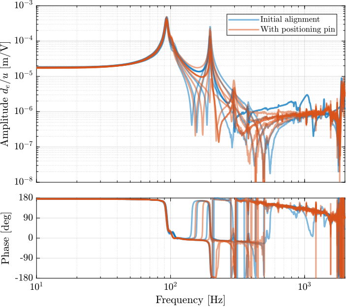
The dynamics of the re-aligned struts are then measured using the same test bench (Figure ref:fig:test_struts_bench_leg). The comparison of the initial strut dynamics and the dynamics of the re-aligned struts (i.e. with the positioning pin) is made in Figure ref:fig:test_struts_comp_enc_frf_realign.

Even though the struts are now much better aligned, not much improvement can be observed. The dynamics of the six aligned struts are quite different from one another.

Having the encoders fixed to the struts may prove to be difficult to use. Therefore, the encoders may be fixed to the nano-hexapod plates instead.

%% New dynamical identified with re-aligned struts
% Load the identification data
leg_noise = {};
for i = 1:length(strut_align_nums)
    leg_noise(i) = {load(sprintf('frf_struts_align_%i_noise.mat', strut_align_nums(i)), 'u', 'Vs', 'de')};
end

% Parameters for Frequency Analysis
Ts = 1e-4; % Sampling Time [s]
Nfft = floor(1/Ts); % Number of points for the FFT computation
win = hanning(Nfft); % Hanning window
Noverlap = floor(Nfft/2); % Overlap between frequency analysis

% Only used to have the frequency vector "f"
[~, f] = tfestimate(leg_noise{1}.u, leg_noise{1}.de, win, Noverlap, Nfft, 1/Ts);

% Transfer function from u to de (encoder)
enc_frf_aligned = zeros(length(f), length(strut_align_nums));

for i = 1:length(strut_align_nums)
    enc_frf_aligned(:, i) = tfestimate(leg_noise{i}.u,    leg_noise{i}.de,    win, Noverlap, Nfft, 1/Ts);
end

Effect of the flexible joint

<<ssec:test_struts_effect_joint_stiffness>>

As the struts are composed of one APA and two flexible joints, it is expected that the flexible joint characteristics will change the dynamic behavior of the struts.

Using the Simscape model, the effect of the flexible joint's characteristics on the dynamics as measured on the test bench are studied. The studied dynamics is between $u$ and the encoder displacement $d_e$.

Let's initialize an APA which is a little bit misaligned.

% APA Initialization
n_hexapod.actuator = initializeAPA('type', 'flexible', 'd_align_bot', [0.1e-3; 0.5e-3; 0], 'd_align_top', [0.1e-3; 0.5e-3; 0]);

%% Study the effect of the bending stiffness of the Flexible joints
% Tested bending stiffnesses [Nm/rad]
kRs = [3, 4, 5, 6, 7];

% Idenfity the transfer function from actuator to encoder for all bending stiffnesses
Gs_kRs = {zeros(length(kRs), 1)};

for i = 1:length(kRs)
    n_hexapod.flex_bot = initializeBotFlexibleJoint(...
        'type', '4dof', ...
        'kRx', kRs(i), ...
        'kRy', kRs(i));
    n_hexapod.flex_top = initializeTopFlexibleJoint(...
        'type', '4dof', ...
        'kRx', kRs(i), ...
        'kRy', kRs(i));

    G = exp(-s*1e-4)*linearize(mdl, io, 0.0, opts);
    G.InputName  = {'u'};
    G.OutputName = {'Vs', 'de', 'da'};

    Gs_kRs(i) = {G};
end

%% Study the effect of the axial stiffness of the Flexible joints
% Tested axial stiffnesses [N/m]
kzs = [5e7 7.5e7 1e8 2.5e8];

% Idenfity the transfer function from actuator to encoder for all bending stiffnesses
Gs_kzs = {zeros(length(kzs), 1)};

for i = 1:length(kzs)
    n_hexapod.flex_bot = initializeBotFlexibleJoint(...
        'type', '4dof', ...
        'kz', kzs(i));
    n_hexapod.flex_top = initializeTopFlexibleJoint(...
        'type', '4dof', ...
        'kz', kzs(i));

    G = exp(-s*1e-4)*linearize(mdl, io, 0.0, opts);
    G.InputName  = {'u'};
    G.OutputName = {'Vs', 'de', 'da'};

    Gs_kzs(i) = {G};
end

The bending stiffness of the joints has little impact on the transfer function from $u$ to $d_e$.

The axial stiffness of the flexible joint has a large impact on the frequency of the complex conjugate zero. Using the measured FRF on the test-bench, if is therefore possible to estimate the axial stiffness of the flexible joints from the location of the zero.

This method gives nice match between the measured FRF and the one extracted from the simscape model, however it could give not so accurate values of the joint's axial stiffness as other factors are also influencing the location of the zero.

Using this method, an axial stiffness of $70 N/\mu m$ is found to give good results (and is reasonable based on the finite element models).

Conclusion   ignore

Conclusion

<<sec:test_struts_conclusion>>

Bibliography   ignore

Footnotes

²Heidenhain MT25, specified accuracy of $\pm 0.5\,\mu m$ ¹Faro Arm Platinum 4ft, specified accuracy of $\pm 13\mu m$

---