phd-test-bench-struts/test-bench-struts.org

Test Bench - Nano-Hexapod Struts

• Glossary and Acronyms - Tables
• Introduction
• Mounting Procedure
• Measurement of flexible modes
• Dynamical measurements
  • Introduction
  • Effect of the Encoder on the measured dynamics
  • Comparison of the encoder and interferometer
  • Comparison of all the Struts
  • Conclusion
• Strut Model
  • Introduction
  • Model dynamics
  • Effect of strut misalignment
  • Measured strut misalignment
  • Proper struts alignment
• Conclusion
• Glossary
• Footnotes

---

This report is also available as a pdf.

---

Glossary and Acronyms - Tables   ignore

key	abbreviation	full form
nass	NASS	Nano Active Stabilization System
fem	FEM	Finite Element Model
apa	APA	Amplified Piezoelectric Actuator
dac	DAC	Digital to Analog Converter

Introduction   ignore

The Nano-Hexapod struts (shown in Figure ref:fig:test_struts_picture_strut) are composed of two flexible joints that are fixed at the two ends of the strut, one acrfull:apa¹ and one optical encoder².

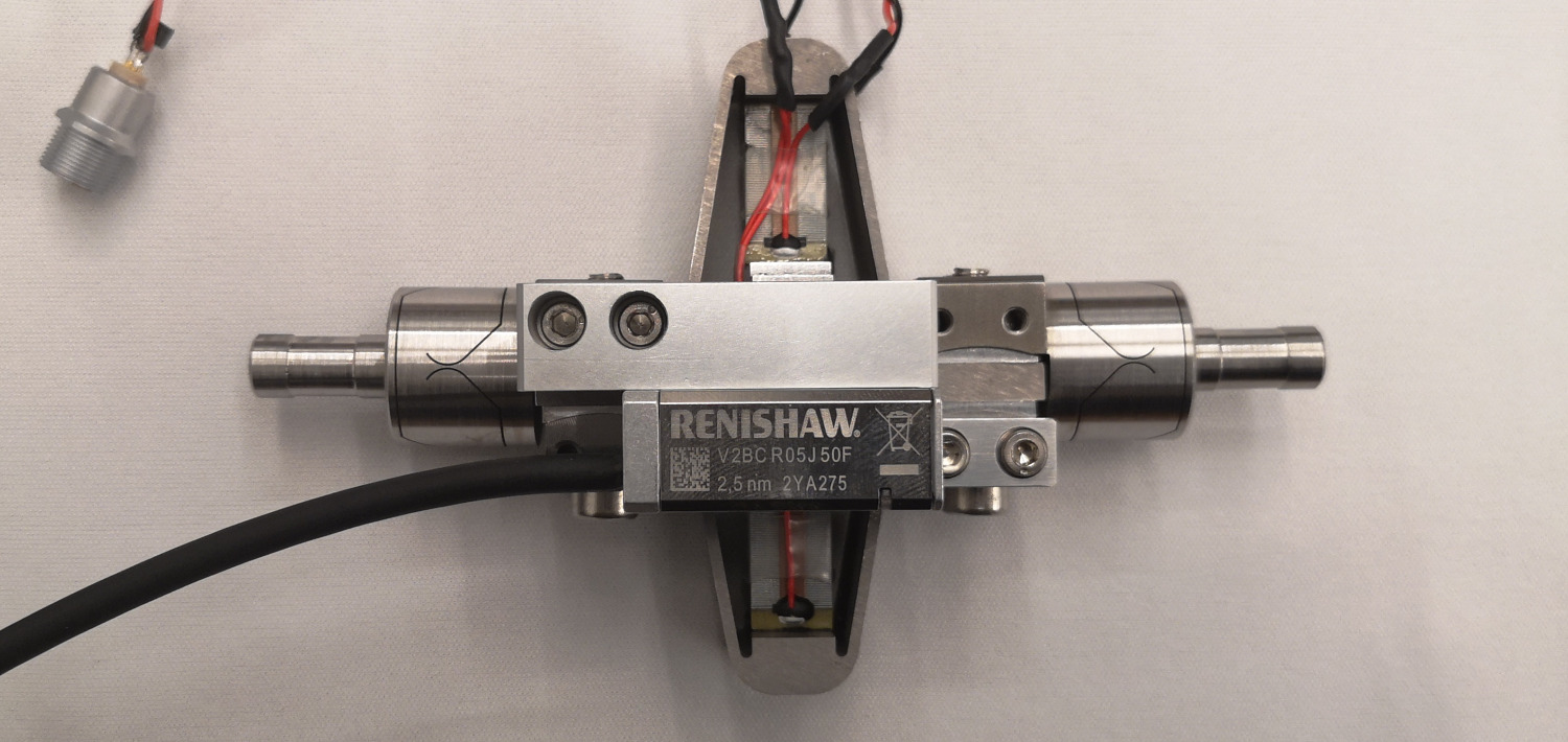
After the strut elements have been individually characterized (see previous sections), the struts are assembled. The mounting procedure of the struts is explained in Section ref:sec:test_struts_mounting. A mounting bench was used to ensure coaxiality between the two ends of the struts. In this way, no angular stroke is lost when mounted to the nano-hexapod.

The flexible modes of the struts were then experimentally measured and compared with a finite element model (Section ref:sec:test_struts_flexible_modes).

Dynamic measurements of the strut are performed with the same test bench used to characterize the APA300ML dynamics (Section ref:sec:test_struts_dynamical_meas). It was found that the dynamics from the acrshort:dac voltage to the displacement measured by the encoder is complex due to the flexible modes of the struts (Section ref:sec:test_struts_flexible_modes).

The strut models were then compared with the measured dynamics (Section ref:sec:test_struts_simscape). The model dynamics from the acrshort:dac voltage to the axial motion of the strut (measured by an interferometer) and to the force sensor voltage well match the experimental results. However, this is not the case for the dynamics from acrshort:dac voltage to the encoder displacement. It is found that the complex dynamics is due to a misalignment between the flexible joints and the acrshort:apa.

Mounting Procedure

<<sec:test_struts_mounting>>

A mounting bench was developed to ensure:

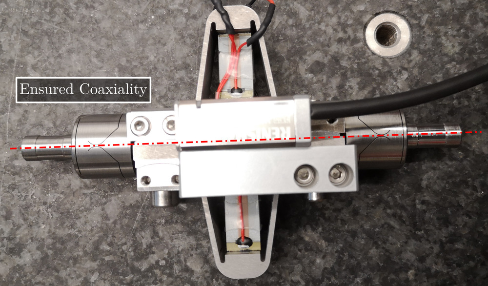
• Good coaxial alignment between the interfaces (cylinders) of the flexible joints. This is important not to loose to much angular stroke during their mounting into the nano-hexapod
• Uniform length across all struts
• Precise alignment of the APA with the two flexible joints
• Reproducible and consistent assembly between all struts

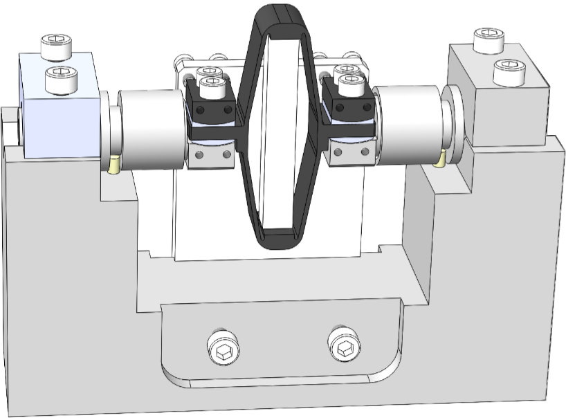
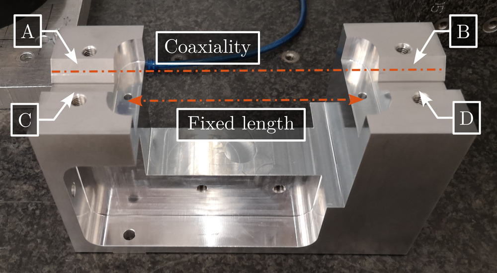
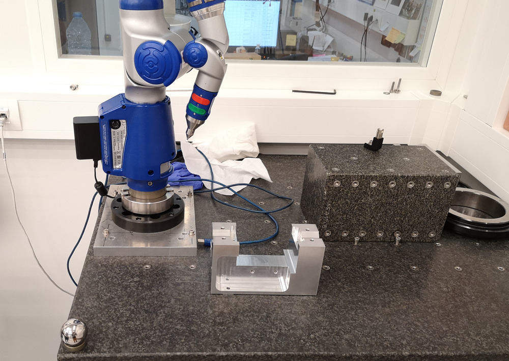
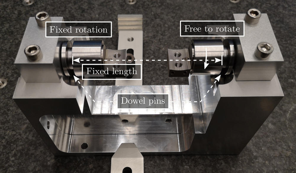
A CAD view of the mounting bench is shown in Figure ref:fig:test_struts_mounting_bench_first_concept. It consists of a "main frame" (Figure ref:fig:test_struts_mounting_step_0) precisely machined to ensure both correct strut length and strut coaxiality. The coaxiality is ensured by good flatness (specified at $20\,\mu m$) between surfaces A and B and between surfaces C and D. Such flatness was checked using a FARO arm³ (see Figure ref:fig:test_struts_check_dimensions_bench) and was found to comply with the requirements. The strut length (defined by the distance between the rotation points of the two flexible joints) was ensured by using precisely machined dowel holes.

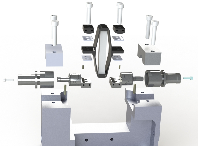
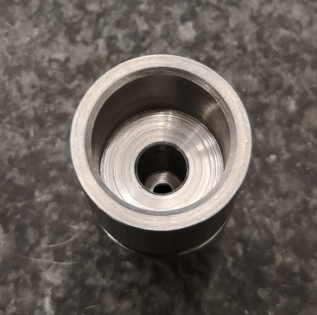
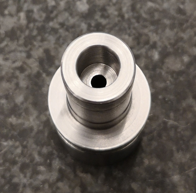
The flexible joints were not directly fixed to the mounting bench but were fixed to a cylindrical "sleeve" shown in Figures ref:fig:test_struts_cylindrical_mounting_part_top and ref:fig:test_struts_cylindrical_mounting_part_bot. The goal of these "sleeves" is to avoid mechanical stress that could damage the flexible joints during the mounting process. These "sleeves" have one dowel groove (that are fitted to the dowel holes shown in Figure ref:fig:test_struts_mounting_step_0) that will determine the length of the mounted strut.

The "sleeves" were mounted to the main element as shown in Figure ref:fig:test_struts_mounting_step_0. The left sleeve has a thigh fit such that its orientation is fixed (it is roughly aligned horizontally), while the right sleeve has a loose fit such that it can rotate (it will get the same orientation as the fixed one when tightening the screws).

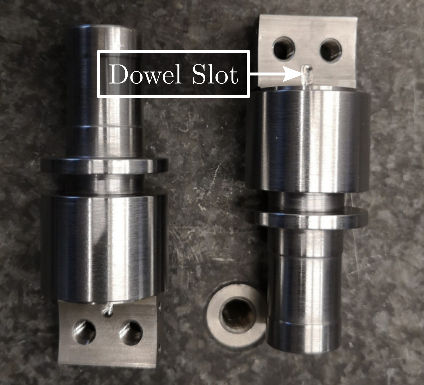
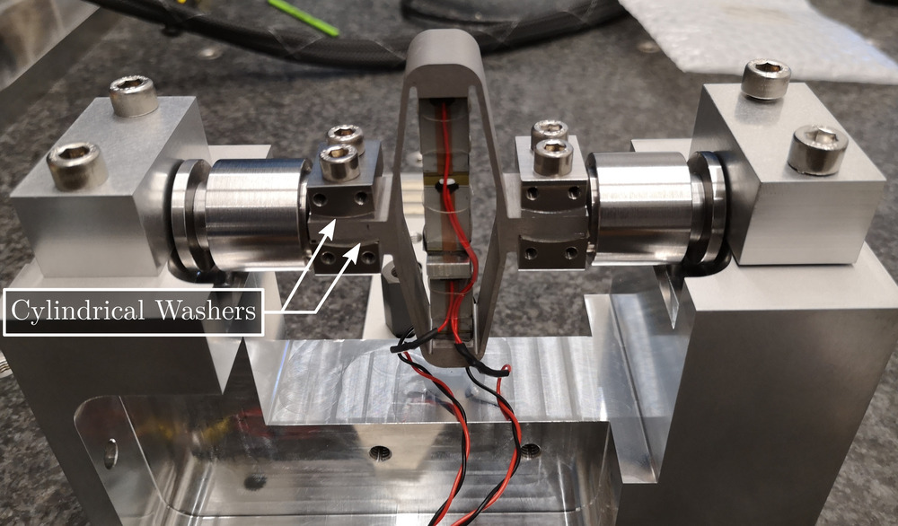
The cylindrical washers and the APA300ML are stacked on top of the flexible joints, as shown in Figure ref:fig:test_struts_mounting_step_2 and screwed together using a torque screwdriver. A dowel pin is used to laterally align the APA300ML with the flexible joints (see the dowel slot on the flexible joints in Figure ref:fig:test_struts_mounting_joints). Two cylindrical washers are used to allow proper mounting even when the two APA interfaces are not parallel.

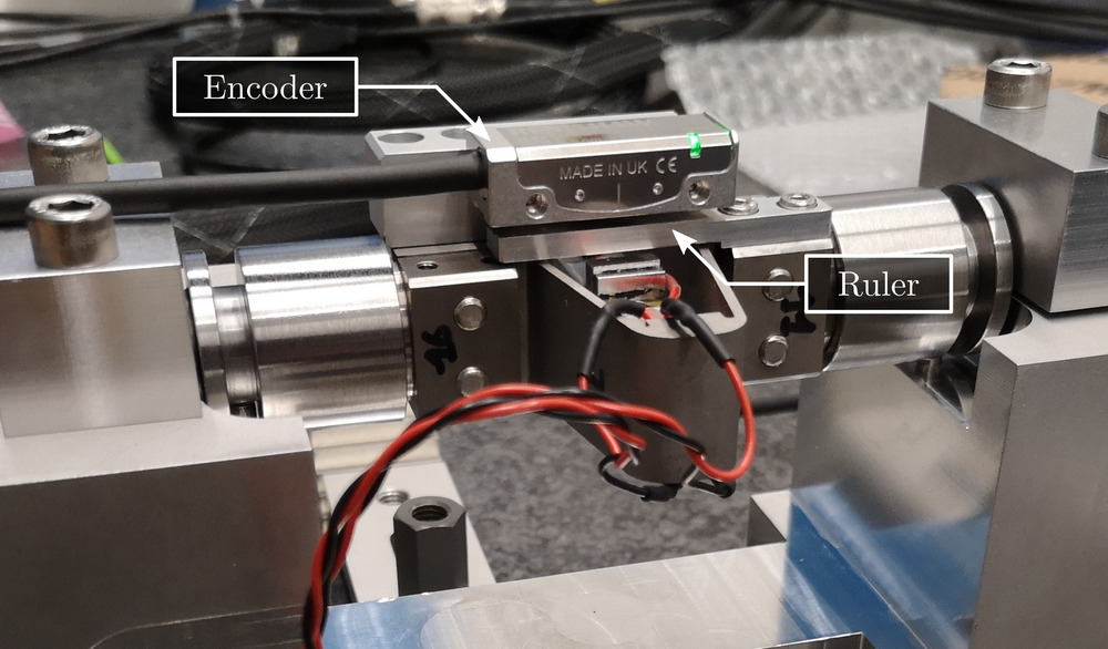
The encoder and ruler are then fixed to the strut and properly aligned, as shown in Figure ref:fig:test_struts_mounting_step_3.

Finally, the strut can be disassembled from the mounting bench (Figure ref:fig:test_struts_mounting_step_4). Thanks to this mounting procedure, the coaxiality and length between the two flexible joint's interfaces can be obtained within the desired tolerances.

\bigskip

Measurement of flexible modes

<<sec:test_struts_flexible_modes>>

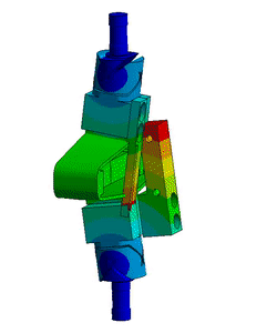
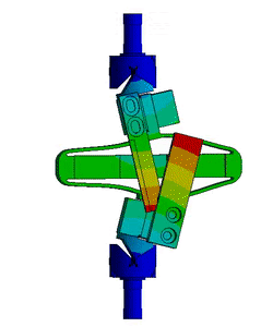
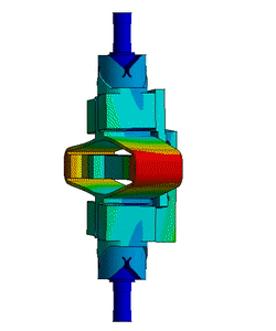
A Finite Element Model⁴ of the struts is developed and is used to estimate the flexible modes. The inertia of the encoder (estimated at $15\,g$) is considered. The two cylindrical interfaces were fixed (boundary conditions), and the first three flexible modes were computed. The mode shapes are displayed in Figure ref:fig:test_struts_mode_shapes: an "X-bending" mode at 189Hz, a "Y-bending" mode at 285Hz and a "Z-torsion" mode at 400Hz.

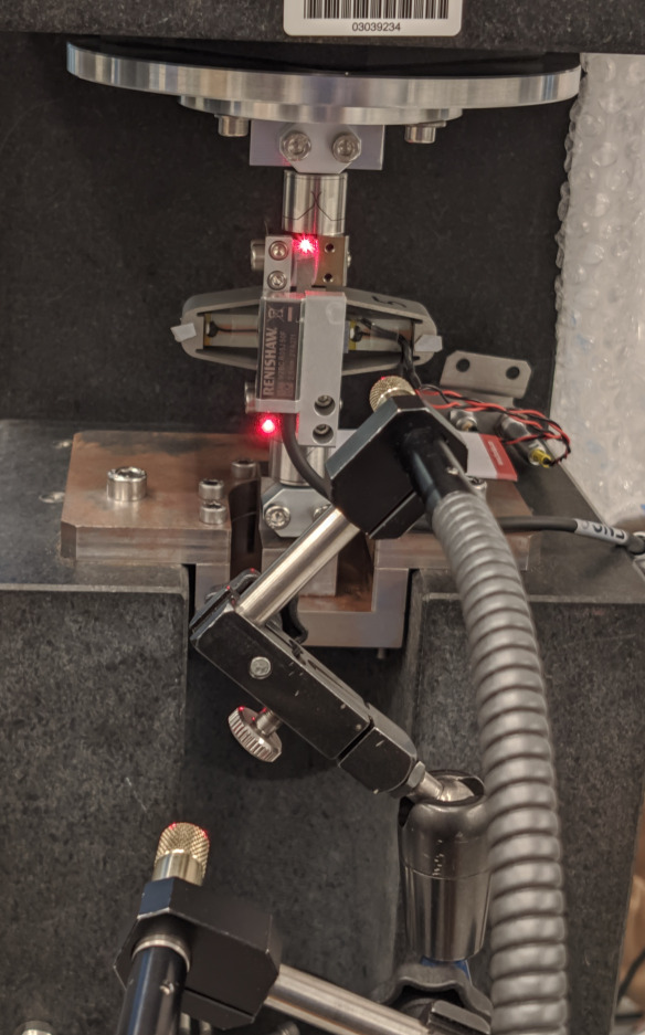
<<m-init-path>>

<<m-init-path-tangle>>

<<m-init-other>>

To experimentally measure these mode shapes, a Laser vibrometer⁵ was used. It measures the difference of motion between two beam path (red points in Figure ref:fig:test_struts_meas_modes). The strut is then excited by an instrumented hammer, and the transfer function from the hammer to the measured rotation is computed.

The setup used to measure the "X-bending" mode is shown in Figure ref:fig:test_struts_meas_x_bending. The "Y-bending" mode is measured as shown in Figure ref:fig:test_struts_meas_y_bending and the "Z-torsion" measurement setup is shown in Figure ref:fig:test_struts_meas_z_torsion. These tests were performed with and without the encoder being fixed to the strut.

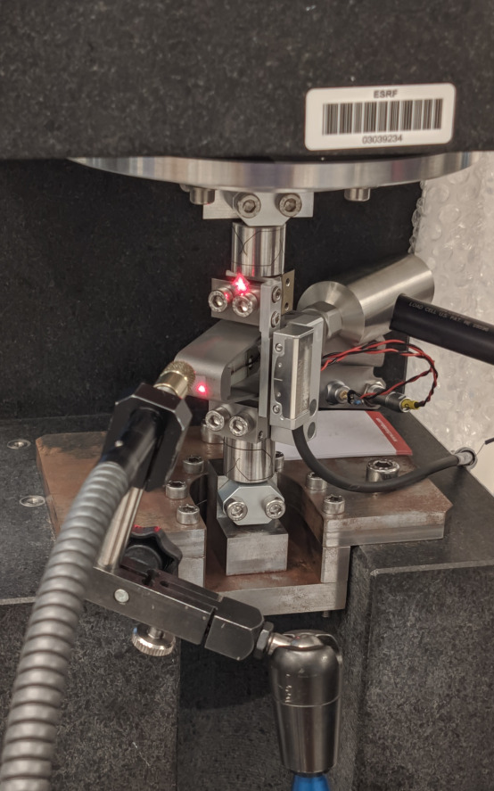
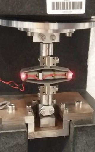
The obtained frequency response functions for the three configurations (X-bending, Y-bending and Z-torsion) are shown in Figure ref:fig:test_struts_spur_res_frf_no_enc when the encoder is not fixed to the strut and in Figure ref:fig:test_struts_spur_res_frf_enc when the encoder is fixed to the strut.

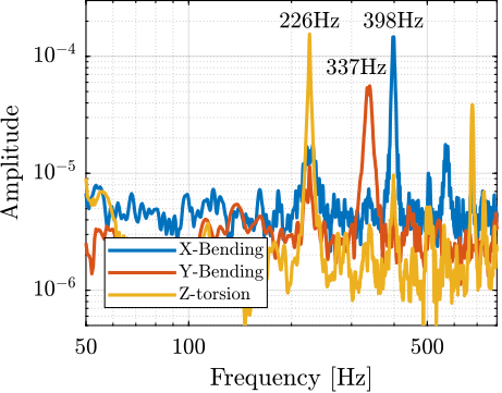
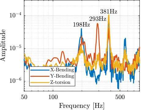
Table ref:tab:test_struts_spur_mode_freqs summarizes the measured resonance frequencies and the computed ones using the acrfull:fem. The resonance frequencies of the 3 modes are only slightly decreased when the encoder is fixed to the strut. In addition, the computed resonance frequencies from the acrshort:fem are very close to the measured frequencies when the encoder is fixed to the strut. This validates the quality of the acrshort:fem.

Mode	FEM with Encoder	Exp. with Encoder	Exp. without Encoder
X-Bending	189Hz	198Hz	226Hz
Y-Bending	285Hz	293Hz	337Hz
Z-Torsion	400Hz	381Hz	398Hz

Dynamical measurements

<<sec:test_struts_dynamical_meas>>

Introduction   ignore

In order to measure the dynamics of the strut, the test bench used to measure the APA300ML dynamics is being used again.

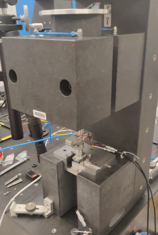
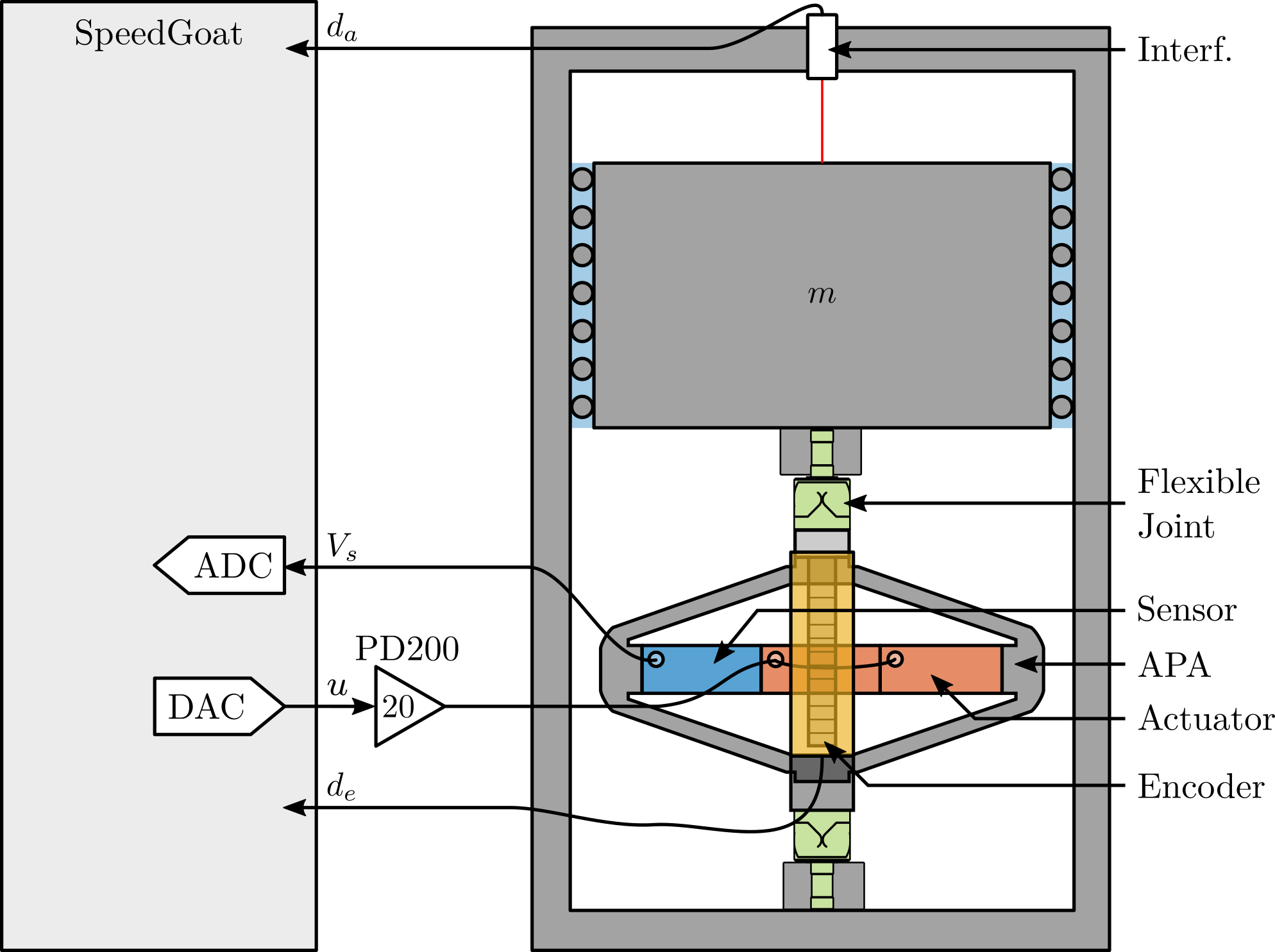
The strut mounted on the bench is shown in Figure ref:fig:test_struts_bench_leg_overview A schematic of the bench and the associated signals are shown in Figure ref:fig:test_struts_bench_schematic. A fiber interferometer⁶ is used to measure the motion of the granite (i.e. the axial motion of the strut).

First, the effect of the encoder on the measured dynamics is investigated in Section ref:ssec:test_struts_effect_encoder. The dynamics observed by the encoder and interferometers are compared in Section ref:ssec:test_struts_comp_enc_int. Finally, all measured struts are compared in terms of dynamics in Section ref:ssec:test_struts_comp_all_struts.

Effect of the Encoder on the measured dynamics

<<ssec:test_struts_effect_encoder>>

%% Parameters for Frequency Analysis
Ts = 1e-4; % Sampling Time [s]
Nfft = floor(1/Ts); % Number of points for the FFT computation
win = hanning(Nfft); % Hanning window
Noverlap = floor(Nfft/2); % Overlap between frequency analysis

%% Measure FRF for Strut 1 - No encoder
% Load Data
leg_sweep    = load('frf_data_leg_1_sweep.mat', 'u', 'Vs', 'de', 'da');
leg_noise_hf = load('frf_data_leg_1_noise_hf.mat', 'u', 'Vs', 'de', 'da');

% We get the frequency vector that will be the same for all the frequency domain analysis.
[~, f] = tfestimate(leg_sweep.u, leg_sweep.de, win, Noverlap, Nfft, 1/Ts);
i_lf = f <= 350; % Indices used for the low frequency
i_hf = f >  350; % Indices used for the high frequency

% Compute FRF function from u to da (interferometer)
[frf_sweep, ~]    = tfestimate(leg_sweep.u,    leg_sweep.da,    win, Noverlap, Nfft, 1/Ts);
[frf_noise_hf, ~] = tfestimate(leg_noise_hf.u, leg_noise_hf.da, win, Noverlap, Nfft, 1/Ts);
int_frf = [frf_sweep(i_lf); frf_noise_hf(i_hf)]; % Combine the FRF

% Compute FRF function from u to Vs (force sensor)
[frf_sweep,    ~] = tfestimate(leg_sweep.u,    leg_sweep.Vs,    win, Noverlap, Nfft, 1/Ts);
[frf_noise_hf, ~] = tfestimate(leg_noise_hf.u, leg_noise_hf.Vs, win, Noverlap, Nfft, 1/Ts);
iff_frf = [frf_sweep(i_lf); frf_noise_hf(i_hf)]; % Combine the FRF

%% Measure FRF for Strut 1 - With encoder
% Load Data
leg_enc_sweep    = load('frf_data_leg_coder_1_noise.mat',    'u', 'Vs', 'de', 'da');
leg_enc_noise_hf = load('frf_data_leg_coder_1_noise_hf.mat', 'u', 'Vs', 'de', 'da');

% Compute FRF function from u to da (interferometer)
[frf_sweep, ~]    = tfestimate(leg_enc_sweep.u,    leg_enc_sweep.da,    win, Noverlap, Nfft, 1/Ts);
[frf_noise_hf, ~] = tfestimate(leg_enc_noise_hf.u, leg_enc_noise_hf.da, win, Noverlap, Nfft, 1/Ts);
int_with_enc_frf = [frf_sweep(i_lf); frf_noise_hf(i_hf)]; % Combine the FRF

% Compute FRF function from u to Vs (force sensor)
[frf_sweep, ~]    = tfestimate(leg_enc_sweep.u,    leg_enc_sweep.Vs,    win, Noverlap, Nfft, 1/Ts);
[frf_noise_hf, ~] = tfestimate(leg_enc_noise_hf.u, leg_enc_noise_hf.Vs, win, Noverlap, Nfft, 1/Ts);
iff_with_enc_frf = [frf_sweep(i_lf); frf_noise_hf(i_hf)]; % Combine the FRF

% Compute FRF function from u to de (encoder)
[frf_sweep, ~]    = tfestimate(leg_enc_sweep.u,    leg_enc_sweep.de,    win, Noverlap, Nfft, 1/Ts);
[frf_noise_hf, ~] = tfestimate(leg_enc_noise_hf.u, leg_enc_noise_hf.de, win, Noverlap, Nfft, 1/Ts);
enc_frf = [frf_sweep(i_lf); frf_noise_hf(i_hf)]; % Combine the FRF

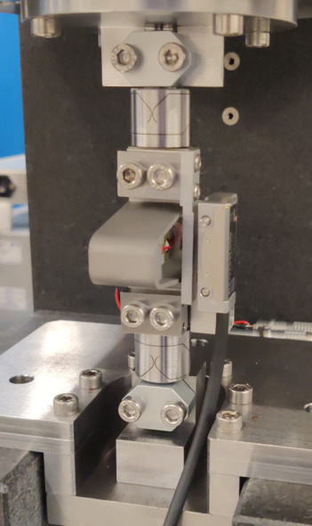
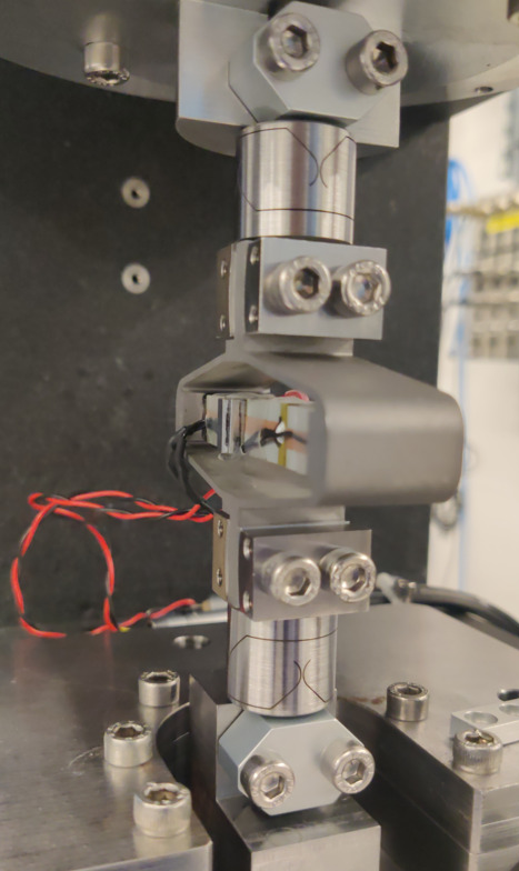
System identification was performed without the encoder being fixed to the strut (Figure ref:fig:test_struts_bench_leg_front) and with one encoder being fixed to the strut (Figure ref:fig:test_struts_bench_leg_coder).

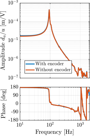
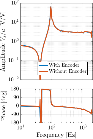
The obtained frequency response functions are compared in Figure ref:fig:test_struts_effect_encoder. It was found that the encoder had very little effect on the transfer function from excitation voltage $u$ to the axial motion of the strut $d_a$ as measured by the interferometer (Figure ref:fig:test_struts_effect_encoder_int). This means that the axial motion of the strut is unaffected by the presence of the encoder. Similarly, it has little effect on the transfer function from $u$ to the sensor stack voltage $V_s$ (Figure ref:fig:test_struts_effect_encoder_iff). This means that the encoder should have little effect on the effectiveness of the integral force feedback control strategy.

Comparison of the encoder and interferometer

<<ssec:test_struts_comp_enc_int>>

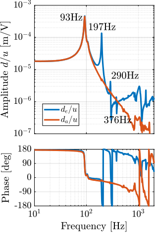
The dynamics measured by the encoder (i.e. $d_e/u$) and interferometers (i.e. $d_a/u$) are compared in Figure ref:fig:test_struts_comp_enc_int. The dynamics from the excitation voltage $u$ to the displacement measured by the encoder $d_e$ presents a behavior that is much more complex than the dynamics of the displacement measured by the interferometer (comparison made in Figure ref:fig:test_struts_comp_enc_int). Three additional resonance frequencies can be observed at 197Hz, 290Hz and 376Hz. These resonance frequencies match the frequencies of the flexible modes studied in Section ref:sec:test_struts_flexible_modes.

The good news is that these resonances are not impacting the axial motion of the strut (which is what is important for the hexapod positioning). However, these resonances make the use of an encoder fixed to the strut difficult from a control perspective.

Comparison of all the Struts

<<ssec:test_struts_comp_all_struts>>

%% Numbers of the measured legs
strut_nums = [1 2 3 4 5];

%% Load the measurement data
% First identification (low frequency noise)
leg_noise = {};
for i = 1:length(strut_nums)
    leg_noise(i) = {load(sprintf('frf_data_leg_coder_%i_noise.mat', strut_nums(i)), 'u', 'Vs', 'de', 'da')};
end

% Second identification (high frequency noise)
leg_noise_hf = {};
for i = 1:length(strut_nums)
    leg_noise_hf(i) = {load(sprintf('frf_data_leg_coder_%i_noise_hf.mat', strut_nums(i)), 'u', 'Vs', 'de', 'da')};
end

%% Compute FRF - From u to de (encoder)
enc_frf = zeros(length(f), length(strut_nums));

for i = 1:length(strut_nums)
    [frf_lf, ~] = tfestimate(leg_noise{i}.u,    detrend(leg_noise{i}.de, 0),    win, Noverlap, Nfft, 1/Ts);
    [frf_hf, ~] = tfestimate(leg_noise_hf{i}.u, detrend(leg_noise_hf{i}.de, 0), win, Noverlap, Nfft, 1/Ts);
    enc_frf(:, i) = [frf_lf(i_lf); frf_hf(i_hf)];
end

%% Compute FRF - From u to da (interferometer)
int_frf = zeros(length(f), length(strut_nums));
for i = 1:length(strut_nums)
    [frf_lf, ~] = tfestimate(leg_noise{i}.u,    leg_noise{i}.da,    win, Noverlap, Nfft, 1/Ts);
    [frf_hf, ~] = tfestimate(leg_noise_hf{i}.u, leg_noise_hf{i}.da, win, Noverlap, Nfft, 1/Ts);
    int_frf(:, i) = [frf_lf(i_lf); frf_hf(i_hf)];
end

%% Compute FRF - From u to Vs (force sensor)
iff_frf = zeros(length(f), length(strut_nums));
for i = 1:length(strut_nums)
    [frf_lf, ~] = tfestimate(leg_noise{i}.u,    leg_noise{i}.Vs,    win, Noverlap, Nfft, 1/Ts);
    [frf_hf, ~] = tfestimate(leg_noise_hf{i}.u, leg_noise_hf{i}.Vs, win, Noverlap, Nfft, 1/Ts);
    iff_frf(:, i) = [frf_lf(i_lf); frf_hf(i_hf)];
end

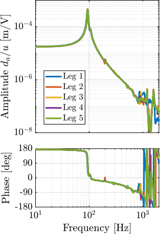
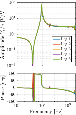
The dynamics of all the mounted struts (only 5 at the time of the experiment) were then measured on the same test bench. The obtained dynamics from $u$ to $d_a$ are compared in Figure ref:fig:test_struts_comp_interf_plants while is dynamics from $u$ to $V_s$ are compared in Figure ref:fig:test_struts_comp_iff_plants. A very good match can be observed between the struts.

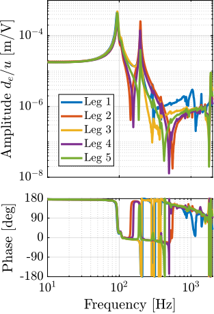
The same comparison is made for the transfer function from $u$ to $d_e$ (encoder output) in Figure ref:fig:test_struts_comp_enc_plants. In this study, large dynamics differences were observed between the 5 struts. Although the same resonance frequencies were seen for all of the struts (95Hz, 200Hz, 300Hz and 400Hz), the amplitude of the peaks were not the same. In addition, the location or even presence of complex conjugate zeros changes from one strut to another.

%% Save the estimated FRF for further analysis
save('./mat/meas_struts_frf.mat', 'f', 'enc_frf', 'int_frf', 'iff_frf', 'strut_nums');

Conclusion

All the struts exhibit very consistent behavior from the excitation voltage $u$ to the force sensor generated voltage $V_s$ and to the interferometer measured displacement $d_a$. However, the dynamics from $u$ to the encoder measurement $d_e$ is much more complex and vary from one strut to the another. The reason for this variability will be studied in the next section thanks to the strut model.

Strut Model

<<sec:test_struts_simscape>>

Introduction   ignore

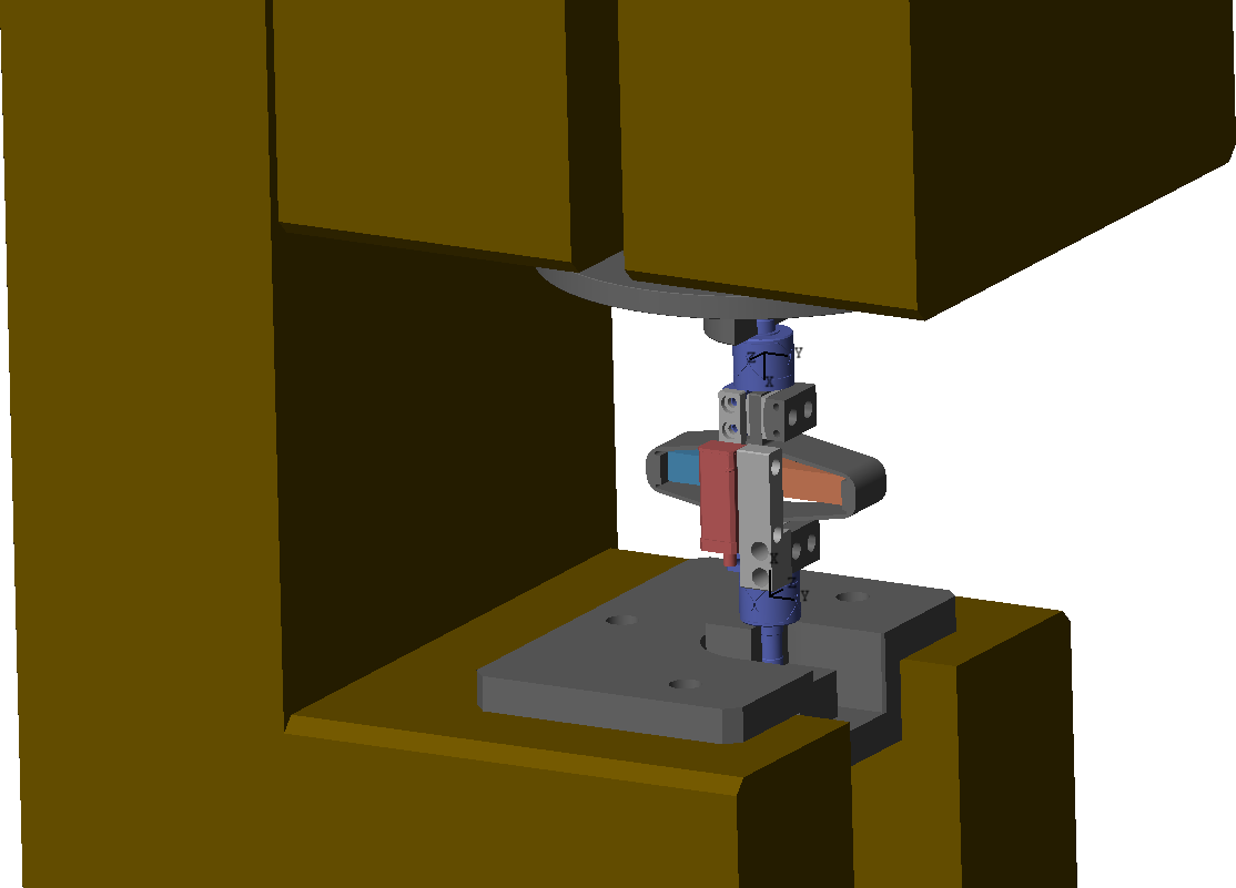
The Simscape model of the strut was included in the Simscape model of the test bench (see Figure ref:fig:test_struts_simscape_model). The obtained model was first used to compare the measured FRF with the existing model (Section ref:ssec:test_struts_comp_model).

Using a flexible APA model (extracted from a acrshort:fem), the effect of a misalignment of the APA with respect to flexible joints is studied (Section ref:ssec:test_struts_effect_misalignment). It was found that misalignment has a large impact on the dynamics from $u$ to $d_e$. This misalignment is estimated and measured in Section ref:ssec:test_struts_meas_misalignment. The struts were then disassembled and reassemble a second time to optimize alignment (Section ref:sec:test_struts_meas_all_aligned_struts).

Model dynamics

<<ssec:test_struts_comp_model>>

%% Load measured FRF for comparison
load('meas_struts_frf.mat', 'f', 'enc_frf', 'int_frf', 'iff_frf', 'strut_nums');

%% Initialize strut with 2DoF model for the APA300ML and identify the dynamics
n_hexapod = struct();
n_hexapod.flex_bot = initializeBotFlexibleJoint('type', '4dof');
n_hexapod.flex_top = initializeTopFlexibleJoint('type', '4dof');
n_hexapod.actuator = initializeAPA('type', '2dof');

c_granite = 0; % Do not take into account damping added by the air bearing

% Run the linearization
Gs_2dof = exp(-s*1e-4)*linearize(mdl, io, 0.0, opts);
Gs_2dof.InputName  = {'u'};
Gs_2dof.OutputName = {'Vs', 'de', 'da'};

%% Initialize strut with "flexible" model for the APA300ML and identify the dynamics
n_hexapod = struct();
n_hexapod.flex_bot = initializeBotFlexibleJoint('type', '4dof');
n_hexapod.flex_top = initializeTopFlexibleJoint('type', '4dof');
n_hexapod.actuator = initializeAPA('type', 'flexible');

c_granite = 100; % Do not take into account damping added by the air bearing

% Run the linearization
Gs_flex = exp(-s*1e-4)*linearize(mdl, io, 0.0, opts);
Gs_flex.InputName  = {'u'};
Gs_flex.OutputName = {'Vs', 'de', 'da'};

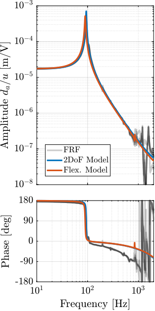
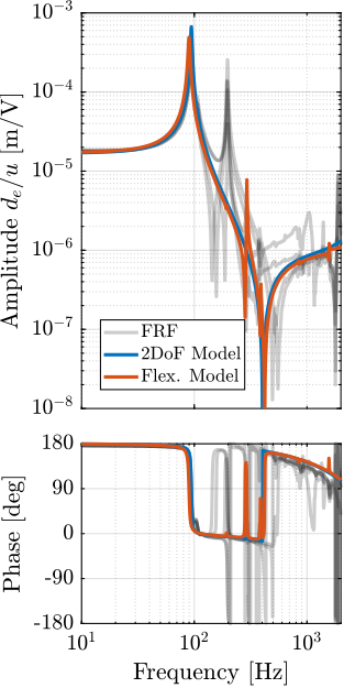
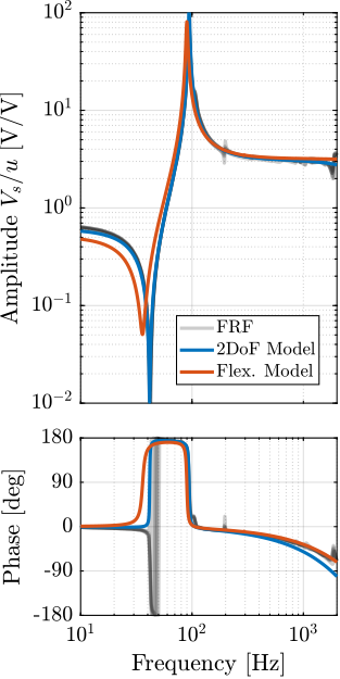
Two models of the APA300ML are used here: a simple two-degrees-of-freedom model and a model using a super-element extracted from a acrlong:fem. These two models of the APA300ML were tuned to best match the measured frequency response functions of the APA alone. The flexible joints were modelled with the 4DoF model (axial stiffness, two bending stiffnesses and one torsion stiffness). These two models are compared with the measured frequency responses in Figure ref:fig:test_struts_comp_frf_flexible_model.

The model dynamics from DAC voltage $u$ to the axial motion of the strut $d_a$ (Figure ref:fig:test_struts_comp_frf_flexible_model_int) and from DAC voltage $u$ to the force sensor voltage $V_s$ (Figure ref:fig:test_struts_comp_frf_flexible_model_iff) are well matching the experimental identification.

However, the transfer function from $u$ to encoder displacement $d_e$ are not well matching for both models. For the 2DoF model, this is normal because the resonances affecting the dynamics are not modelled at all (the APA300ML is modeled as infinitely rigid in all directions except the translation along it's actuation axis). For the flexible model, it will be shown in the next section that by adding some misalignment between the flexible joints and the APA300ML, this model can better represent the observed dynamics.

Effect of strut misalignment

<<ssec:test_struts_effect_misalignment>>

As shown in Figure ref:fig:test_struts_comp_enc_plants, the identified dynamics from DAC voltage $u$ to encoder measured displacement $d_e$ are very different from one strut to the other. In this section, it is investigated whether poor alignment of the strut (flexible joints with respect to the APA) can explain such dynamics. For instance, consider Figure ref:fig:test_struts_misalign_schematic where there is a misalignment in the $y$ direction between the two flexible joints (well aligned thanks to the mounting procedure in Section ref:sec:test_struts_mounting) and the APA300ML. In this case, the "x-bending" mode at 200Hz (see Figure ref:fig:test_struts_meas_x_bending) can be expected to have greater impact on the dynamics from the actuator to the encoder.

To verify this assumption, the dynamics from the output DAC voltage $u$ to the measured displacement by the encoder $d_e$ is computed using the flexible APA Simscape model for several misalignments in the $y$ direction. The obtained dynamics are shown in Figure ref:fig:test_struts_effect_misalignment_y. The alignment of the APA with the flexible joints has a large influence on the dynamics from actuator voltage to the measured displacement by the encoder. The misalignment in the $y$ direction mostly influences:

• the presence of the flexible mode at 200Hz (see mode shape in Figure ref:fig:test_struts_mode_shapes_1)

• the location of the complex conjugate zero between the first two resonances:

  • if $d_{y} < 0$: there is no zero between the two resonances and possibly not even between the second and third resonances
  • if $d_{y} > 0$: there is a complex conjugate zero between the first two resonances
• the location of the high frequency complex conjugate zeros at 500Hz (secondary effect, as the axial stiffness of the joint also has large effect on the position of this zero)

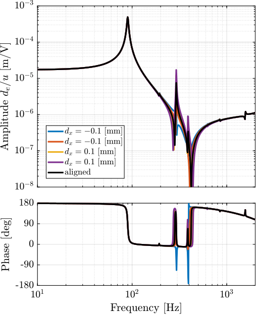
The same can be done for misalignments in the $x$ direction. The obtained dynamics (Figure ref:fig:test_struts_effect_misalignment_x) are showing that misalignment in the $x$ direction mostly influences the presence of the flexible mode at 300Hz (see mode shape in Figure ref:fig:test_struts_mode_shapes_2).

A comparison of the experimental frequency response functions in Figure ref:fig:test_struts_comp_enc_plants with the model dynamics for several $y$ misalignments in Figure ref:fig:test_struts_effect_misalignment_y indicates a clear similarity. This similarity suggests that the identified differences in dynamics are caused by misalignment.

%% Effect of a misalignment in Y-Direction
% Considered misalignment in the Y direction
dy_aligns = [-0.5, -0.1, 0.1, 0.5]*1e-3; % [m]

% Transfer functions from u to de for all the misalignment in y direction
Gs_dy_align = {zeros(length(dy_aligns), 1)};

for i = 1:length(dy_aligns)
    n_hexapod.actuator = initializeAPA('type', 'flexible', 'd_align_bot', [0; dy_aligns(i); 0], 'd_align_top', [0; dy_aligns(i); 0]);

    G = exp(-s*1e-4)*linearize(mdl, io, 0.0, opts);
    G.InputName  = {'u'};
    G.OutputName = {'Vs', 'de', 'da'};

    Gs_dy_align(i) = {G};
end

%% Effect of a misalignment in X-Direction
% Considered misalignment in the X direction
dx_aligns = [-0.1, -0.05, 0.05, 0.1]*1e-3; % [m]

% Transfer functions from u to de for all the misalignment in x direction
Gs_dx_align = {zeros(length(dx_aligns), 1)};

for i = 1:length(dx_aligns)
    n_hexapod.actuator = initializeAPA('type', 'flexible', 'd_align_bot', [dx_aligns(i); 0; 0], 'd_align_top', [dx_aligns(i); 0; 0]);

    G = exp(-s*1e-4)*linearize(mdl, io, 0.0, opts);
    G.InputName  = {'u'};
    G.OutputName = {'Vs', 'de', 'da'};

    Gs_dx_align(i) = {G};
end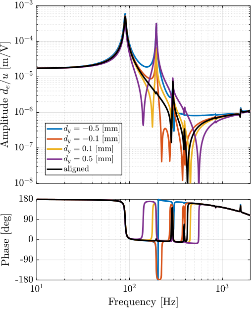

Measured strut misalignment

<<ssec:test_struts_meas_misalignment>>

During the initial mounting of the struts, as presented in Section ref:sec:test_struts_mounting, the positioning pins that were used to position the APA with respect to the flexible joints in the $y$ directions were not used (not received at the time). Therefore, large $y$ misalignments are expected.

To estimate the misalignments between the two flexible joints and the APA:

• the struts were fixed horizontally on the mounting bench, as shown in Figure ref:fig:test_struts_mounting_step_3 but without the encoder
• using a length gauge⁷, the height difference between the flexible joints surface and the APA shell surface was measured for both the top and bottom joints and for both sides
• as the thickness of the flexible joint is $21\,mm$ and the thickness of the APA shell is $20\,mm$, $0.5\,mm$ of height difference should be measured if the two are perfectly aligned

Large variations in the $y$ misalignment are found from one strut to the other (results are summarized in Table ref:tab:test_struts_meas_y_misalignment).

To check the validity of the measurement, it can be verified that the sum of the measured thickness difference on each side is $1\,mm$ (equal to the thickness difference between the flexible joint and the APA). Thickness differences for all the struts were found to be between $0.94\,mm$ and $1.00\,mm$ which indicate low errors compared to the misalignments found in Table ref:tab:test_struts_meas_y_misalignment.

%% Measurement of the y misalignment between the APA and the flexible joints
% Mesured struts
strut_nums = [1, 2, 3, 4, 5];

% Measured height differences in [mm]
% R ("red" side), B ("black" side)
%                R Top  B Top  R Bot  B Bot
strut_align = [[-0.40, -0.60, -0.16, -0.82]   % Strut 1
               [-0.67, -0.30, -0.34, -0.63]   % Strut 2
               [-0.07, -0.88, -0.16, -0.79]   % Strut 3
               [-0.48, -0.46,  0.07, -1.00]   % Strut 4
               [-0.33, -0.64, -0.48, -0.52]]; % Strut 5

% Verification that the thickness difference between the APA shell and the flexible joints is 1mm
thichness_diff_top = strut_align(:,1) + strut_align(:,2); % [mm]
thichness_diff_bot = strut_align(:,1) + strut_align(:,2); % [mm]

% Estimation of the dy misalignment
dy_bot = (strut_align(:,1) - strut_align(:,2))/2; % [mm]
dy_top = (strut_align(:,3) - strut_align(:,4))/2; % [mm]

Strut	Bot	Top
1	0.1	0.33
2	-0.19	0.14
3	0.41	0.32
4	-0.01	0.54
5	0.15	0.02

By using the measured $y$ misalignment in the Simscape model with the flexible APA model, the model dynamics from $u$ to $d_e$ is closer to the measured dynamics, as shown in Figure ref:fig:test_struts_comp_dy_tuned_model_frf_enc. A better match in the dynamics can be obtained by fine-tuning both the $x$ and $y$ misalignments (yellow curves in Figure ref:fig:test_struts_comp_dy_tuned_model_frf_enc).

This confirms that misalignment between the APA and the strut axis (determined by the two flexible joints) is critical and inducing large variations in the dynamics from DAC voltage $u$ to encoder measured displacement $d_e$. If encoders are fixed to the struts, the APA and flexible joints must be precisely aligned when mounting the struts.

In the next section, the struts are re-assembled with a "positioning pin" to better align the APA with the flexible joints. With a better alignment, the amplitude of the spurious resonances is expected to decrease, as shown in Figure ref:fig:test_struts_effect_misalignment_y.

%% Idenfity the dynamics from u to de - misalignement estimated from measurement
Gs_y_align = {zeros(size(strut_align,1), 1)};

% Measured dy alignment
strut_align = 1e-3*[[-0.60, -0.82, -0.40, -0.16]
                    [-0.30, -0.63, -0.67, -0.34]
                    [-0.88, -0.79, -0.07, -0.16]
                    [-0.48,  0.07, -0.46, -1.00]
                    [-0.33, -0.48, -0.64, -0.52]
                    [-0.34, -0.42, -0.63, -0.57]];

for i = 1:size(strut_align,1)
    n_hexapod.actuator = initializeAPA('type', 'flexible', ...
                                       'd_align_bot', [0; strut_align(i, 2) - strut_align(i, 4); 0], ...
                                       'd_align_top', [0; strut_align(i, 1) - strut_align(i, 3); 0]);

    G = exp(-s*1e-4)*linearize(mdl, io, 0.0, opts);
    G.InputName  = {'u'};
    G.OutputName = {'Vs', 'de', 'da'};

    Gs_y_align(i) = {G};
end

%% Idenfity the dynamics from u to de - misalignement tuned to have the best match
d_aligns = [[-0.05,  -0.3,  0];
            [ 0,      0.5,  0];
            [-0.1,   -0.3,  0];
            [ 0,      0.3,  0];
            [-0.05,   0.05, 0]]'*1e-3;

% Idenfity the transfer function from actuator to encoder for all cases
Gs_xy_align = {zeros(size(d_aligns,2), 1)};

for i = 1:5
    n_hexapod.actuator = initializeAPA('type', 'flexible', 'd_align_top', d_aligns(:,i), 'd_align_bot', d_aligns(:,i));

    G = exp(-s*1e-4)*linearize(mdl, io, 0.0, opts);
    G.InputName  = {'u'};
    G.OutputName = {'Vs', 'de', 'da'};

    Gs_xy_align(i) = {G};
end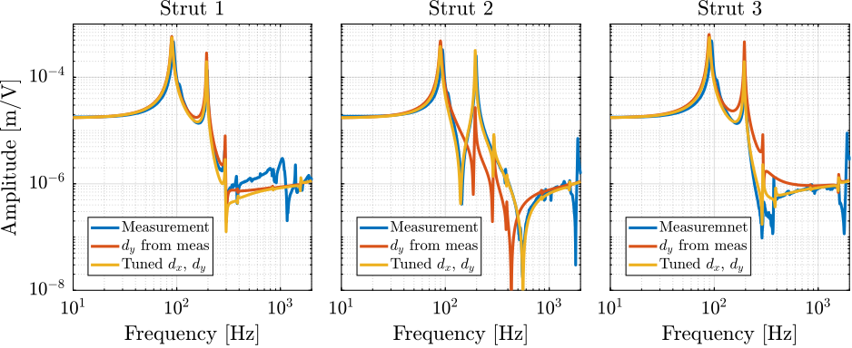

Comparison of the frequency response functions from DAC voltage $u$ to measured displacement $d_e$ by the encoders for the three struts. In blue, the measured dynamics is represted, in red the dynamics extracted from the model with the $y$ misalignment estimated from measurements, and in yellow, the dynamics extracted from the model when both the $x$ and $y$ misalignments are tuned

Proper struts alignment

<<sec:test_struts_meas_all_aligned_struts>>

After receiving the positioning pins, the struts were mounted again with the positioning pins. This should improve the alignment of the APA with the two flexible joints.

The alignment is then estimated using a length gauge, as described in the previous sections. Measured $y$ alignments are summarized in Table ref:tab:test_struts_meas_y_misalignment_with_pin and are found to be bellow $55\mu m$ for all the struts, which is much better than before (see Table ref:tab:test_struts_meas_y_misalignment).

%% Measurement of the y misalignment between the APA and the flexible joints after strut better alignment

% Numbers of the measured legs
strut_align_nums = [1 2 3 4 5 6];

% Measured height differences in [mm]
% R ("red" side), B ("black" side)
%                R Top  B Top  R Bot  B Bot
strut_align = [[-0.54, -0.50, -0.50, -0.52]   % strut 1
               [-0.44, -0.55, -0.49, -0.49]   % strut 2
               [-0.48, -0.50, -0.50, -0.46]   % strut 3
               [-0.45, -0.51, -0.51, -0.45]   % strut 4
               [-0.50, -0.50, -0.50, -0.50]   % strut 5
               [-0.50, -0.49, -0.43, -0.54]]; % strut 6

% Verification that the thickness difference between the APA shell and the flexible joints is 1mm
thichness_diff_top = strut_align(:,1) + strut_align(:,2); % [mm]
thichness_diff_bot = strut_align(:,1) + strut_align(:,2); % [mm]

% Estimation of the dy misalignment
dy_bot = (strut_align(:,1) - strut_align(:,2))/2; % [mm]
dy_top = (strut_align(:,3) - strut_align(:,4))/2; % [mm]

Strut	Bot	Top
1	-0.02	0.01
2	0.055	0.0
3	0.01	-0.02
4	0.03	-0.03
5	0.0	0.0
6	-0.005	0.055

The dynamics of the re-aligned struts were then measured on the same test bench (Figure ref:fig:test_struts_bench_leg). A comparison of the initial strut dynamics and the dynamics of the re-aligned struts (i.e. with the positioning pin) is presented in Figure ref:fig:test_struts_comp_enc_frf_realign. Even though the struts are now much better aligned, not much improvement can be observed. The dynamics of the six aligned struts were also quite different from one another.

The fact that the encoders are fixed to the struts makes the control more challenging. Therefore, fixing the encoders to the nano-hexapod plates instead may be an interesting option.

%% New dynamical identified with re-aligned struts
% Load the identification data
leg_noise = {};
for i = 1:length(strut_align_nums)
    leg_noise(i) = {load(sprintf('frf_struts_align_%i_noise.mat', strut_align_nums(i)), 'u', 'Vs', 'de')};
end

% Parameters for Frequency Analysis
Ts = 1e-4; % Sampling Time [s]
Nfft = floor(1/Ts); % Number of points for the FFT computation
win = hanning(Nfft); % Hanning window
Noverlap = floor(Nfft/2); % Overlap between frequency analysis

% Only used to have the frequency vector "f"
[~, f] = tfestimate(leg_noise{1}.u, leg_noise{1}.de, win, Noverlap, Nfft, 1/Ts);

% Transfer function from u to de (encoder)
enc_frf_aligned = zeros(length(f), length(strut_align_nums));

for i = 1:length(strut_align_nums)
    enc_frf_aligned(:, i) = tfestimate(leg_noise{i}.u,    leg_noise{i}.de,    win, Noverlap, Nfft, 1/Ts);
end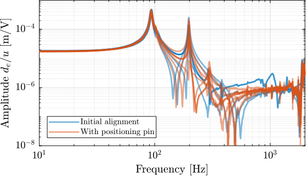

Comparison of the dynamics from $u$ to $d_e$ before and after proper alignment using the dowel pins

Conclusion

<<sec:test_struts_conclusion>>

The Hano-Hexapod struts are a key component of the developed acrfull:nass. A mounting bench was used to obtain struts with good interface coaxiality, equal lengths, and ideally the same dynamics. Using a test bench, it was found that while all the mounted struts had extremely similar dynamics when considering the axial motion and the integrated force sensor, the dynamics as seen by the encoder is much more complex and varied from one strut to the other.

Thanks to a acrshort:fem and experimental measurements, the modes inducing this complex dynamics was identified. The variability in the dynamics was attributed to the poor alignment of the acrshort:apa with respect to the flexible joints. Even with better alignment using dowel pins, the observed dynamics by the encoder remained problematic. Therefore, the encoders will be fixed directly to the nano-hexapod plates rather than being fixed to the struts.

Glossary   ignore

printglossaries:

Footnotes

---

¹

APA300ML from Cedrat Technologies

²

Vionic from Renishaw

³

FARO Arm Platinum 4ft, specified accuracy of $\pm 13\mu m$

⁴

Using Ansys\textsuperscript{\textregistered}. Flexible Joints and APA Shell are made of a stainless steel allow called 17-4 PH. Encoder and ruler support material is aluminium.

⁵

OFV-3001 controller and OFV512 sensor head from Polytec

⁶

Two fiber intereferometers were used: an IDS3010 from Attocube and a quDIS from QuTools

⁷

Heidenhain MT25, specified accuracy of $\pm 0.5\,\mu m$