phd-test-bench-spindle/test-bench-nass-spindle.org

Nano-Hexapod on top of a Spindle - Test Bench

• Introduction
• Test-Bench Description
  • Introduction
  • Alignment
  • Short Range metrology system
  • Spindle errors
    • Introduction
    • Errors in $D_x$ and $D_y$
    • Errors in vertical motion $D_z$
    • Angle errors in $R_x$ and $R_y$
• Simscape Model
  • Introduction
  • Simscape model parameters
  • Control Architecture
  • Computation of the strut errors from the external metrology
  • IFF Plant
  • DVF Plant
  • HAC Plant
• Control Experiment
  • IFF Plant
  • IFF Controller
  • Open Loop Plant
  • Damped Plant
  • HAC Controller
  • Compare dynamics seen by interferometers and by encoders
  • Compare dynamics obtained with different Rz estimations
• Closed-Loop Results
  • Open and Closed loop results

Introduction   ignore

As the different beamlines are running 24/7 It is difficult to have access to the micro station to perform tests. The only slot available is 3 weeks during the summer.

Before the tests on ID31:

• Development of a 5DoF metrology system
• Make sure all the kinematic is working properly

Test-Bench Description

Introduction   ignore

Here are the documentation of the equipment used for this test bench:

• Voltage Amplifier: PiezoDrive PD200
• Amplified Piezoelectric Actuator: Cedrat APA300ML
• DAC/ADC: Speedgoat IO131
• Encoder: Renishaw Vionic and used Ruler
• LION Precision CPL290
• Spindle: Lab Motion RT250S with Drivebox 3.6 controller

Alignment

Procedure:

1. Align bottom sphere with the spindle rotation axis (~ 10um)
2. Align top sphere with the spindle rotation axis (~ 10um)

Short Range metrology system

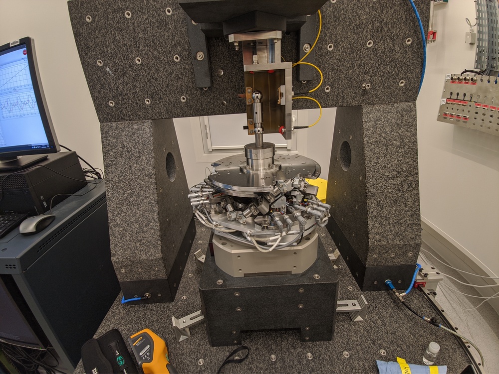
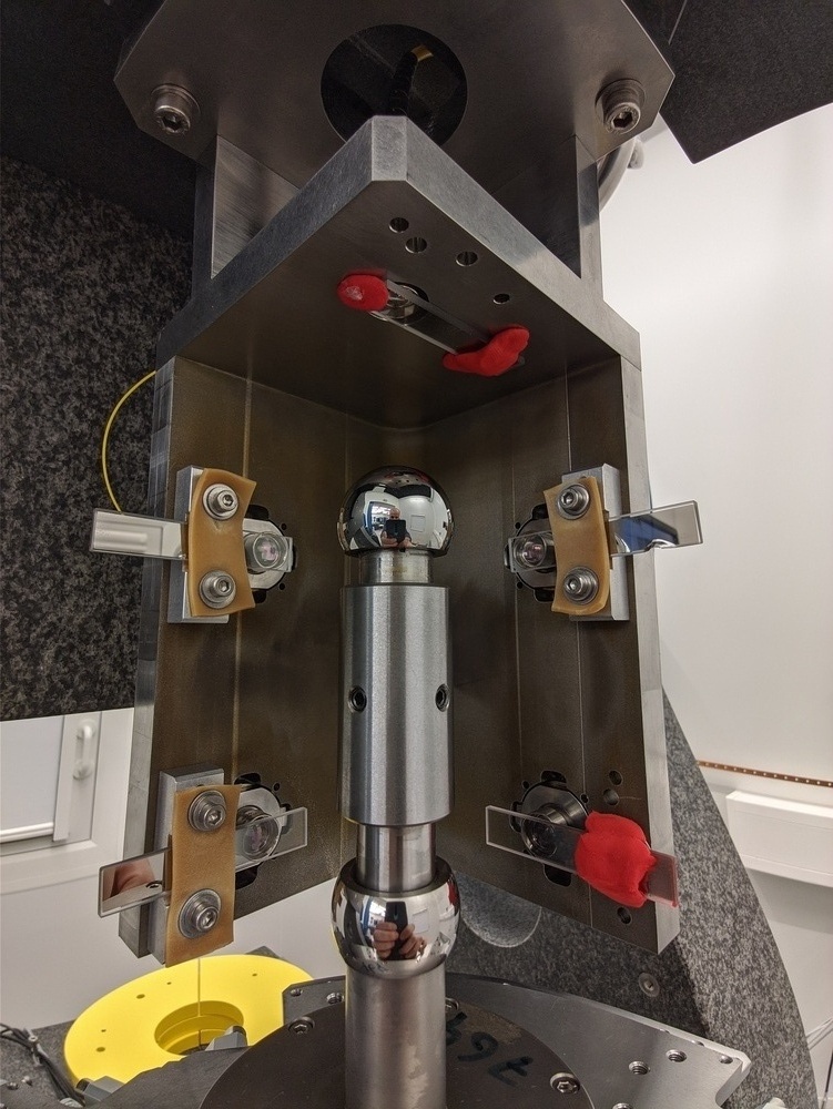
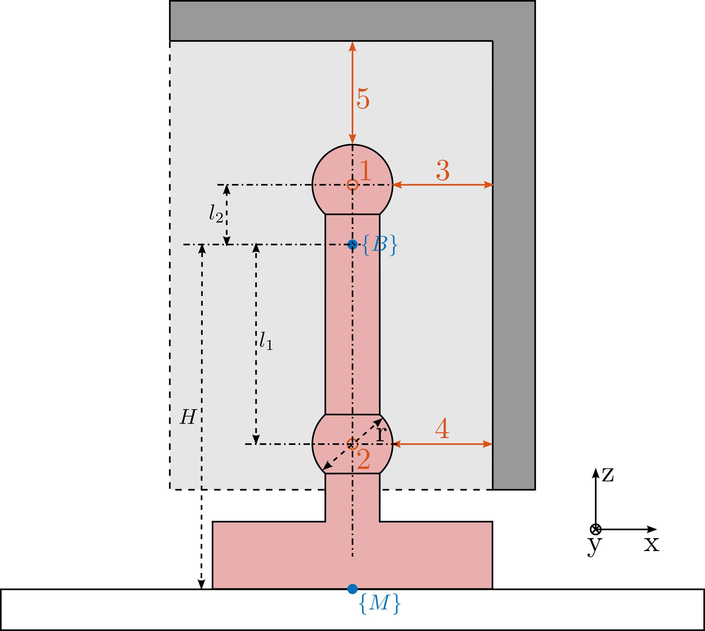
There are 5 interferometers pointing at 2 spheres as shown in Figure ref:fig:LION_metrology_interferometers.

	Value
Sphere Diameter	25.4mm
Distance between the spheres	76.2mm

Assumptions:

• Interferometers are perfectly positioned / oriented
• Sphere is perfect

Compute the Jacobian matrix:

• From pure X-Y-Z-Rx-Ry small motions, compute the effect on the 5 measured distances
• Compute the matrix
• Inverse the matrix
• Verify that it is working with simple example (for example using Solidworkds)

We have the following set of equations:

\begin{align} d_1 &= -D_y + l_2 R_x \\ d_2 &= -D_y - l_1 R_x \\ d_3 &= -D_x - l_2 R_y \\ d_4 &= -D_x + l_1 R_y \\ d_5 &= -D_z \end{align}

That can be written as a linear transformation:

\begin{equation} \begin{bmatrix} d_1 \\ d_2 \\ d_3 \\ d_4 \\ d_5 \end{bmatrix} = \begin{bmatrix} 0 & -1 & 0 & l_2 & 0 \\ 0 & -1 & 0 & -l_1 & 0 \\ -1 & 0 & 0 & 0 & -l_2 \\ -1 & 0 & 0 & 0 & l_1 \\ 0 & 0 & -1 & 0 & 0 \end{bmatrix} \cdot \begin{bmatrix} D_x \\ D_y \\ D_z \\ R_x \\ R_y \end{bmatrix} \end{equation}

By inverting the matrix, we obtain the Jacobian relation:

\begin{equation} \begin{bmatrix} D_x \\ D_y \\ D_z \\ R_x \\ R_y \end{bmatrix} = \begin{bmatrix} 0 & -1 & 0 & l_2 & 0 \\ 0 & -1 & 0 & -l_1 & 0 \\ -1 & 0 & 0 & 0 & -l_2 \\ -1 & 0 & 0 & 0 & l_1 \\ 0 & 0 & -1 & 0 & 0 \end{bmatrix}^{-1} \cdot \begin{bmatrix} d_1 \\ d_2 \\ d_3 \\ d_4 \\ d_5 \end{bmatrix} \end{equation}

%% Parameters
H = 150e-3;
l1 = (150-38-52)*1e-3;
l2 = (52+38+76.2-150)*1e-3;

%% Transformation matrix
Hm = [ 0 -1  0  l2  0;
       0 -1  0 -l1  0;
      -1  0  0  0  -l2;
      -1  0  0  0   l1;
       0  0 -1  0   0];

	d1	d2	d3	d4	d5
Dx	0.0	0.0	-0.79	-0.21	0.0
Dy	-0.79	-0.21	-0.0	-0.0	0.0
Dz	0.0	0.0	0.0	0.0	-1.0
Rx	13.12	-13.12	0.0	-0.0	0.0
Ry	0.0	0.0	-13.12	13.12	0.0

Spindle errors

Introduction   ignore

The spindle is rotated at 60rpm during 10 turns. The signal of all 5 interferometers are recorded.

data = load(sprintf('%s/spindle/mat/2022-12-20_15-47_sec_test.mat', data_dir));

Errors in $D_x$ and $D_y$

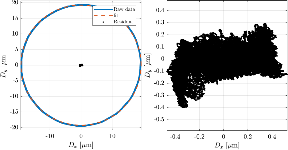
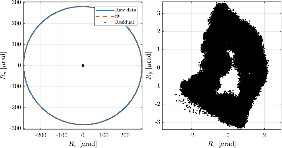
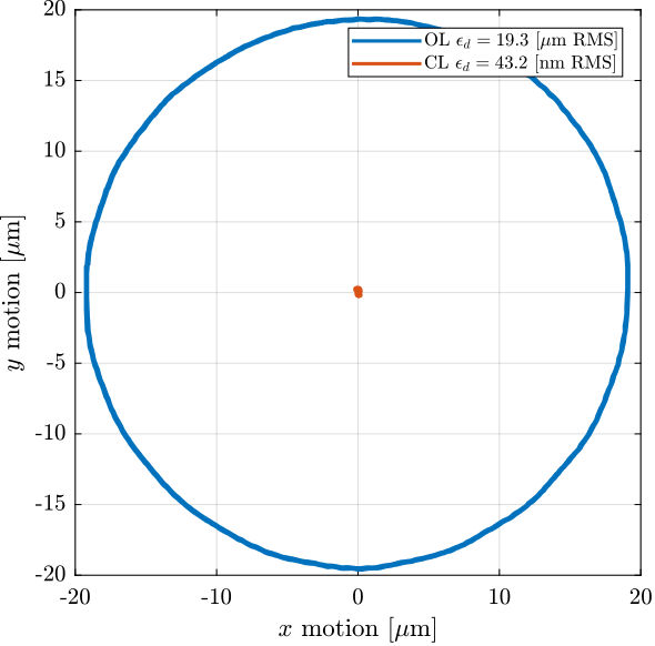
Because of the eccentricity of the reference surfaces (the spheres), we expect the motion in the X-Y plane to be a circle as a first approximation. We can first see that in Figure ref:fig:dx_dy_motion_rotation that shows the measured $D_x$ and $D_y$ motion as a function of the $R_z$ angle.

Dx and Dy motion during the rotation

%% Circle Fit
[xc,yc,R,a] = circlefit(data.Dx_int, data.Dy_int);

A circle is fit, and the obtained radius of the circle (i.e. the excentricity) is estimated to be:

Error linked to excentricity = 19 um

The motion in the X-Y plane as well as the circle fit and the residual motion (circle fit subtracted from the measured motion) are shown in Figure ref:fig:dx_dy_spindle_rotation.

Dx and Dy motion during the spindle rotation

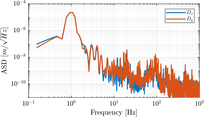
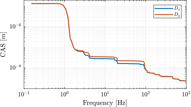
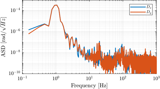
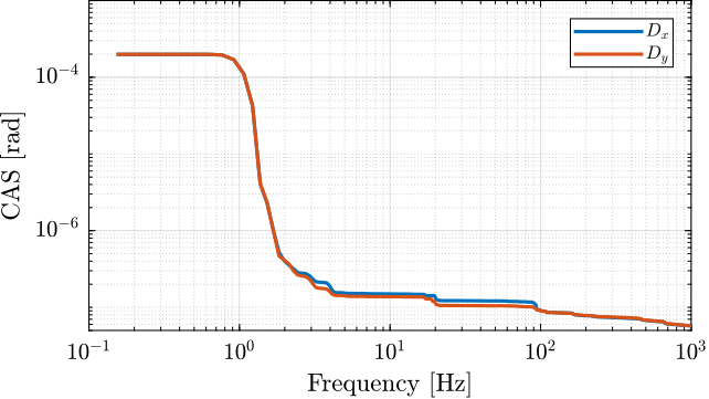
Let's now analyse the frequency content in the signal.

Amplitude Spectral Density of the measured Dx and Dy motion

Cumulative Amplitude Spectrum of the measured Dx and Dy motion

Errors in vertical motion $D_z$

The top interferometer is measuring the vertical motion of the sphere.

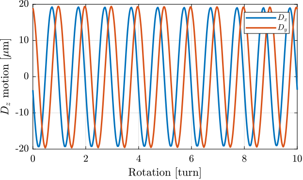
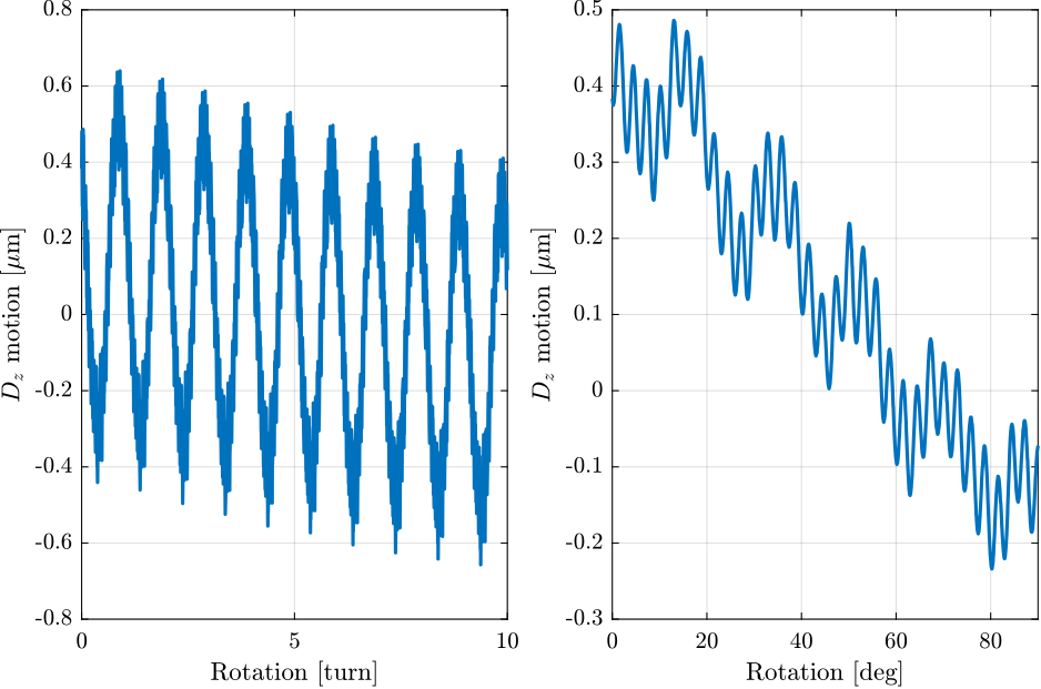
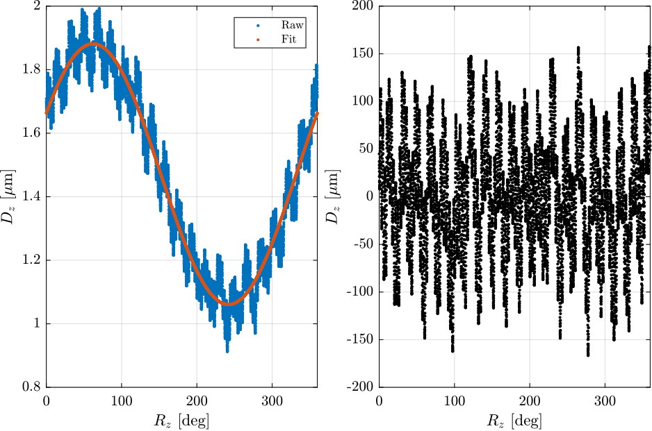
However, if the top sphere is not perfectly aligned with the spindle axis, there will also measure some vertical motion due to this excentricity.

Dz motion during the rotation

Let's fit a sinus with a period of one turn.

%% Fit Sinus with period of one turn
x1 = data.Rz(data.t<1);
y1 = data.Dz_int(data.t<1);

fit = @(b,x)  b(1).*sin(x + b(2)) + b(3);    % Function to fit
fcn = @(b) sum((fit(b,x1) - y1).^2);                             % Least-Squares cost function

s1 = fminsearch(fcn, [1e-6;  30;  1.5e-6])                      % Minimise Least-Squares

Errors linked to excentricity = 410 [nm]

Effect of the excentricity and remaining Dz motion

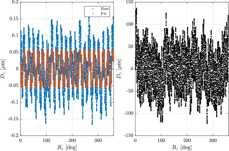
If we look at the remaining motion after removing the effect of the eccentricity (Figure ref:fig:dz_motion_rotation_excentricity, right), we can see a signal with 20 periods every turn. Let's fit this.

%% Fit Sinus with period of 18 degrees (one electrical period)
x2 = data.Rz(data.t<1)*20;
y2 = y1 - fit(s1, x1);

fit = @(b,x)  b(1).*sin(x + b(2)) + b(3);    % Function to fit
fcn = @(b) sum((fit(b,x2) - y2).^2);                             % Least-Squares cost function

s2 = fminsearch(fcn, [50e-9;  30;  0])                      % Minimise Least-Squares

Errors linked to spindle motor = 58 [nm]

Effect of the magnetic pole pairs and remaining Dz motion

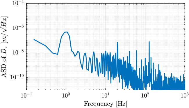
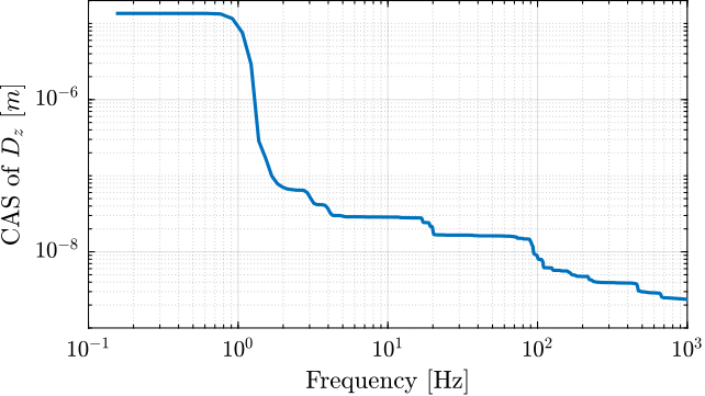
Let's look at the signal in the frequency domain.

On top of the peak at 1Hz (excentricity) and at 20Hz (number of pole pairs), we can observe a frequency of 126Hz (i.e. 126 periods per turn, approx 2.85 deg).

Could this be related to the air bearing system?

Amplitude Spectral Density of the measured Dz motion

Cumulative Amplitude Spectrum of the measured Dz motion

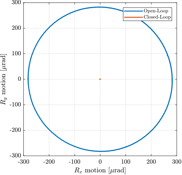
Angle errors in $R_x$ and $R_y$

[xc,yc,R,a] = circlefit(data.Rx_int, data.Ry_int);

amplitude = 281 urad

Rx and Ry motion during the spindle rotation

Let's now analyse the frequency content in the signal.

Amplitude Spectral Density of the measured Rx and Ry motion

Cumulative Amplitude Spectrum of the measured Rx and Ry motion

Simscape Model

Introduction   ignore

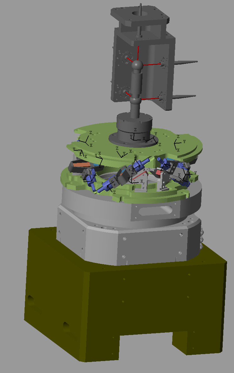
A 3D view of the Simscape model is shown in Figure ref:fig:simscape_model_spindle_bench. The Spindle is represented by a Bushing joint. Axial, radial and tilt stiffnesses are taken from the Spindle datasheet (see Table).

Stiffness	Value	Unit
Axial	402	$N/\mu m$
Radial	226	$N/\mu m$
Tilt	2380	$Nm/mrad$

The metrology system consists of 5 distance measurements (represented by the red lines in Figure ref:fig:simscape_model_spindle_bench).

Simscape model parameters

The nano-hexapod is initialized.

%% Initialize Nano-Hexapod
n_hexapod = initializeNanoHexapodFinal('MO_B', 150e-3, ...
                                       'actuator_type', '2dof', ...
                                       'motion_sensor_type', 'plates');

%% Initialize Spindle
spindle = struct();

%% Stiffnesses
spindle.kx = 226e6; % Radial stiffness in [N/m]
spindle.ky = 226e6; % Radial stiffness in [N/m]
spindle.kz = 402e6; % Axial stiffness in [N/m]
spindle.krx = 2.38e6; % Tilt stiffness in [Nm/rad]
spindle.kry = 2.38e6; % Tilt stiffness in [Nm/rad]
spindle.krz = 0; % Rotation stiffness in [Nm/rad]

%% Damping
spindle.cx = 1/(2*0.01)/(sqrt(spindle.kx*50)); % Radial damping in [N/(m/s)]
spindle.cy = 1/(2*0.01)/(sqrt(spindle.ky*50)); % Radial damping in [N/(m/s)]
spindle.cz = 1/(2*0.01)/(sqrt(spindle.kz*50)); % Axial damping in [N/(m/s)]
spindle.crx = 1/(2*0.01)/(sqrt(spindle.krx*50)); % Tilt damping in [Nm/(rad/s)]
spindle.cry = 1/(2*0.01)/(sqrt(spindle.kry*50)); % Tilt damping in [Nm/(rad/s)]
spindle.crz = 0; % Rotation damping in [Nm/(rad/s)]

The Jacobian matrix that computes the $[x, y, z, R_x, R_y]$ motion of the sample from the 5 interferometers is defined below.

% Sensor Jacobian (Interferometers to Cartesian motion)
J_int_to_X_ = [ 0                 0                -0.787401574803149 -0.212598425196851  0;
               -0.78740157480315 -0.21259842519685  0                  0                  0;
                0                 0                 0                  0                 -1;
               13.1233595800525 -13.1233595800525   0                  0                  0;
                0                 0               -13.1233595800525   13.1233595800525    0];

Control Architecture

Let's note:

• $d\mathcal{L}_m = [d_{\mathcal{L}_1},\ d_{\mathcal{L}_2},\ d_{\mathcal{L}_3},\ d_{\mathcal{L}_4},\ d_{\mathcal{L}_5},\ d_{\mathcal{L}_6}]$ the measurement of the 6 encoders fixed to the nano-hexapod
• $\bm{\tau}_m = [\tau_{m_1},\ \tau_{m_2},\ \tau_{m_3},\ \tau_{m_4},\ \tau_{m_5},\ \tau_{m_6}]$ the voltages measured by the 6 force sensors
• $\bm{u} = [u_1,\ u_2,\ u_3,\ u_4,\ u_5,\ u_6]$ the voltages send to the voltage amplifiers for the 6 piezoelectric actuators
• $R_z$ the spindle measured angle (encoder)
• $\bm{d}_m = [d_1,\ d_2,\ d_3,\ d_4,\ d_5]$ the distances measured by the 5 interferometers (see Figure ref:fig:LION_metrology_interferometers_bis)

Computation of the strut errors from the external metrology

The following frames are defined:

• $\{ W \}$: the frame that represents the wanted pose of the sample
• $\{ M \}$: the frame that represents the measured pose of the sample (estimated from the 5 interferometers and the spindle encoder)
• $\{ G \}$: the frame fixed to the granite and positioned at the sample's center
• $\{ H \}$: the frame fixed to the the spindle rotor, and positioned at the sample's center

We can express several homogeneous transformation matrices.

Frame fixed to the spindle rotor (centered on the sample's position), expressed in the frame of the granite:

\begin{equation} {}^{G}\bm{T}_H = \begin{bmatrix} cos(R_z) & -sin(R_z) & 0 & 0 \\ sin(R_z) & cos(R_z) & 0 & 0 \\ 0 & 0 & 1 & 0 \\ 0 & 0 & 0 & 1 \end{bmatrix} \end{equation}

with $R_z$ the spindle encoder.

Wanted position expressed in the frame of the granite:

\begin{equation} {}^{G}\bm{T}_W = \begin{bmatrix} & & & r_{D_x} \\ & \bm{R}_x(r_{R_x}) \bm{R}_y(r_{R_y}) \bm{R}_z(r_{R_z}) & & r_{D_y} \\ & & & r_{D_z} \\ 0 & 0 & 0 & 1 \end{bmatrix} \end{equation}

with $\bm{R}(r_{R_x}, r_{R_y}, r_{R_z})$ representing the wanted orientation of the sample with respect to the granite. Typically, $r_{R_x} = 0$, $r_{R_y} = 0$ and $r_{R_z}$ corresponds to the spindle encoder $R_z$.

Measured position of the sample with respect to the granite:

\begin{equation} {}^{G}\bm{T}_M = \begin{bmatrix} & & & y_{D_x} \\ & \bm{R}_x(y_{R_x}) \bm{R}_y(y_{R_y}) \bm{R}_z(R_z) & & y_{D_y} \\ & & & y_{D_z} \\ 0 & 0 & 0 & 1 \end{bmatrix} \end{equation}

with $R_z$ the spindle encoder, and $[y_{D_x},\ y_{D_y},\ y_{D_z},\ y_{R_x},\ y_{R_y}]$ are obtained from the 5 interferometers:

\begin{equation} \begin{bmatrix} y_{D_x} \\ y_{D_y} \\ y_{D_z} \\ y_{R_x} \\ y_{R_y} \end{bmatrix} = \begin{bmatrix} 0 & -1 & 0 & l_2 & 0 \\ 0 & -1 & 0 & -l_1 & 0 \\ -1 & 0 & 0 & 0 & -l_2 \\ -1 & 0 & 0 & 0 & l_1 \\ 0 & 0 & -1 & 0 & 0 \end{bmatrix}^{-1} \cdot \begin{bmatrix} d_1 \\ d_2 \\ d_3 \\ d_4 \\ d_5 \end{bmatrix} \end{equation}

In order to have the position error in the frame of the nano-hexapod, we have to compute ${}^M\bm{T}_W$:

\begin{align} {}^M\bm{T}_W &= {}^M\bm{T}_G \cdot {}^G\bm{T}_W \\ &= {{}^G\bm{T}_M}^{-1} \cdot {}^G\bm{T}_W \end{align}

The inverse of the transformation matrix can be obtained by

\begin{equation} {}^B\bm{T}_A = {}^A\bm{T}_B^{-1} = \left[ \begin{array}{ccc|c} & & & \\ & {}^A\bm{R}_B^T & & -{}^A \bm{R}_B^T {}^A\bm{P}_{O_B} \\ & & & \cr \hline 0 & 0 & 0 & 1 \\ \end{array} \right] \end{equation}

The position errors $\bm{\epsilon}_{\mathcal{X}} = [\epsilon_{D_x},\ \epsilon_{D_y},\ \epsilon_{D_z},\ \epsilon_{R_x},\ \epsilon_{R_y},\ \epsilon_{R_z}]$ expressed in a frame fixed to the nano-hexapod can be extracted from ${}^W\bm{T}_M$:

• $\epsilon_{D_x} = {}^M\bm{T}_W(1,4)$
• $\epsilon_{D_y} = {}^M\bm{T}_W(2,4)$
• $\epsilon_{D_z} = {}^M\bm{T}_W(3,4)$
• $\epsilon_{R_y} = \text{atan2}({}^M\bm{T}_W(1,3), \sqrt{{}^M\bm{T}_W(1,1)^2 + {}^M\bm{T}_W(1,2)^2})$
• $\epsilon_{R_x} = \text{atan2}(\frac{-{}^M\bm{T}_W(2,3)}{\cos(\epsilon_{R_y})}, \frac{{}^M\bm{T}_W(3,3)}{\cos(\epsilon_{R_y})})$
• $\epsilon_{R_z} = \text{atan2}(\frac{-{}^M\bm{T}_W(1,2)}{\cos(\epsilon_{R_y})}, \frac{{}^M\bm{T}_W(1,1)}{\cos(\epsilon_{R_y})})$

Finally, the strut errors $\bm{\epsilon}_{\mathcal{L}} = [\epsilon_{\matcal{L}_1},\ \epsilon_{\matcal{L}_2},\ \epsilon_{\matcal{L}_3},\ \epsilon_{\matcal{L}_4},\ \epsilon_{\matcal{L}_5},\ \epsilon_{\matcal{L}_6}]$ can be computed from:

\begin{equation} \bm{\epsilon}_\mathcal{L} = \bm{J} \cdot \bm{\epsilon}_\mathcal{X} \end{equation}

IFF Plant

start_angle = 0; % [deg]

options = linearizeOptions;
options.SampleTime = 0;

%% Identify the transfer function from u to taum
clear io; io_i = 1;
io(io_i) = linio([mdl, '/F'],  1, 'openinput');   io_i = io_i + 1; % Actuator Inputs
io(io_i) = linio([mdl, '/Fm'], 1, 'openoutput'); io_i = io_i + 1;  % Force Sensors

%% Perform the model extraction
G_iff = linearize(mdl, io, 0.0, options);

DVF Plant

start_angle = 0; % [deg]

options = linearizeOptions;
options.SampleTime = 0;

%% Identify the transfer function from u to taum
clear io; io_i = 1;
io(io_i) = linio([mdl, '/F'],  1, 'openinput');   io_i = io_i + 1; % Actuator Inputs
io(io_i) = linio([mdl, '/dL'], 1, 'openoutput'); io_i = io_i + 1;  % Encoders

%% Perform the model extraction
G_dvf = linearize(mdl, io, 0.0, options);

HAC Plant

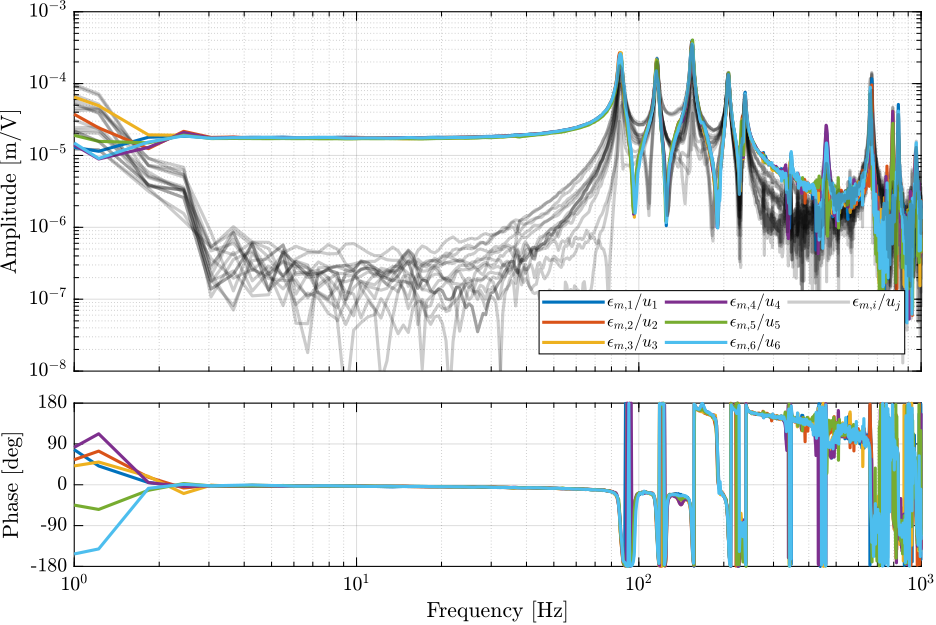
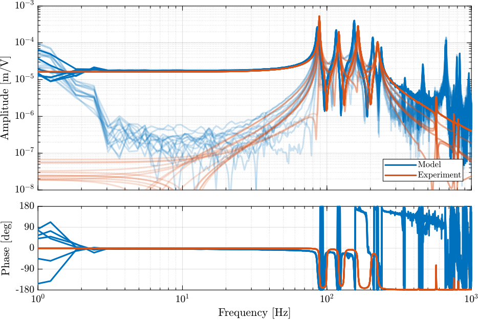
The transfer functions from the 6 actuator inputs to the 6 estimated strut errors are extracted from the Simscape model.

start_angle = 0; % [deg]

options = linearizeOptions;
options.SampleTime = 0;

%% Identify the transfer function from u to taum
clear io; io_i = 1;
io(io_i) = linio([mdl, '/F'],  1, 'openinput');   io_i = io_i + 1; % Actuator Inputs
io(io_i) = linio([mdl, '/J_X_to_L'],  1, 'openoutput'); io_i = io_i + 1; % Estimated Strut Error

%% Perform the model extraction
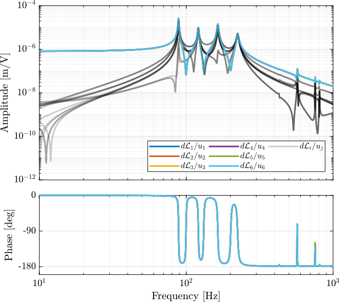
G = linearize(mdl, io, 0.0, options);

The obtained transfer functions are shown in Figure ref:fig:simscape_model_hac_plant.

We can see that the system is well decoupled at low frequency (i.e. below the first resonance of the Nano-Hexapod).

HAC plant obtained on the Simscape model

Control Experiment

IFF Plant

%% Load identification data
data = load(sprintf('%s/dynamics/2023-02-01_15-21_identification_new_matrices_long_bis.mat', data_path));

Obtained transfer function from generated voltages to measured voltages on the piezoelectric force sensor

Comparison with the model

IFF Controller

%% IFF Controller
Kiff_g1 = -(1/(s + 2*pi*40))*...    % LPF: provides integral action above 40Hz
           (s/(s + 2*pi*30))*...    % HPF: limit low frequency gain
           (1/(1 + s/2/pi/500))*... % LPF: more robust to high frequency resonances
           eye(6);                  % Diagonal 6x6 controller

Root Locus for IFF

Open Loop Plant

Here the $R_z$ motion of the Hexapod is estimated from the encoders.

Obtained transfer function from generated voltages to estimated strut motion

Comparison of the open-loop plant measured experimentally and extracted from Simscape

Damped Plant

%% Load identification data for the damped plant
data = load(sprintf('%s/dynamics/2023-02-01_16-04_identification_damped_iff_long.mat', data_path));

Obtained transfer function from generated voltages to estimated strut motion

Comparison of the undamped and damped plant with IFF

HAC Controller

%% Lead to increase phase margin
a  = 4;  % Amount of phase lead / width of the phase lead / high frequency gain
wc = 2*pi*15; % Frequency with the maximum phase lead [rad/s]

H_lead = (1 + s/(wc/sqrt(a)))/(1 + s/(wc*sqrt(a)));

%% Low Pass filter to increase robustness
H_lpf = 1/(1 + s/2/pi/60);

%% Notch at the top-plate resonance
gm = 0.02;
xi = 0.3;
wn = 2*pi*665;

H_notch = (s^2 + 2*gm*xi*wn*s + wn^2)/(s^2 + 2*xi*wn*s + wn^2);

%% Decentralized HAC
Khac_iff_struts = (8e3) * ... % Gain
                  H_notch * ...      % Notch
                  H_lpf * ...      % LPF
                  (2*pi*100/s) * ... % Integrator
                  eye(6);            % 6x6 Diagonal

Loop gain for the HAC

Obtained Root Locus

Compare dynamics seen by interferometers and by encoders

Comparison of the identified dynamic by the internal metrology (encoders) and by the external metrology (interferometers)

Compare dynamics obtained with different Rz estimations

Comparison of the obtained plant using the Encoders or using the output Voltages to estimate Rz

Closed-Loop Results

Open and Closed loop results

data_ol = load(sprintf('%s/spindle/2022-12-20_15-43_sec_test.mat', data_path));
data_cl = load(sprintf('%s/spindle/2023-02-01_16-57_closed_loop.mat', data_path));

Comparison of the Open-Loop and Closed-Loop spindle errors

Comparison of the Open-Loop and Closed-Loop spindle errors - Rotation