phd-test-bench-id31/test-bench-id31.org

Nano-Hexapod on the micro-station

• Introduction
• Short Stroke Metrology System
  • Introduction
  • Metrology Kinematics
  • Rough alignment of the reference spheres
  • Tip-Tilt adjustment of the interferometers
  • Fine Alignment of reference spheres using interferometers
  • Estimated measurement volume
  • Estimated measurement errors
• Identified Open Loop Plant
  • Introduction
  • First Open-Loop Plant Identification
  • Better Angular Alignment
  • Open-Loop Identification after alignment
  • Effect of Payload Mass
  • Effect of Spindle Rotation
  • Identification of Spurious modes
  • Conclusion
• Decentralized Integral Force Feedback
  • Introduction
  • IFF Plant
  • IFF Controller
  • Estimated Damped Plant
  • Conclusion
• High Authority Control in the frame of the struts
  • Introduction
  • Damped Plant
  • Robust Controller Design
  • Estimation of performances
  • Robustness to change of payload
  • Conclusion
• Bibliography
• Footnotes

---

This report is also available as a pdf.

---

Introduction   ignore

Now that the nano-hexapod is mounted and that a good multi-body model of the nano-hexapod The system is validated on the ID31 beamline.

At the beginning of the project, it was planned to develop a long stroke 5-DoF metrology system to measure the pose of the sample with respect to the granite. The development of such system was complex, and was not completed at the time of the experimental tests on ID31. To still validate the developed nano active platform and the associated instrumentation and control architecture, a 5-DoF short stroke metrology system was developed (Section ref:sec:test_id31_metrology).

The identify dynamics of the nano-hexapod fixed on top of the micro-station was identified for different experimental conditions (payload masses, rotational velocities) and compared with the model (Section ref:sec:test_id31_open_loop_plant).

Decentralized Integral Force Feedback is then applied to actively damp the plant in a robust way (Section ref:sec:test_id31_iff).

High authority control is then applied (Section ref:sec:test_id31_iff_hac).

Short Stroke Metrology System

<<sec:test_id31_metrology>>

Introduction   ignore

The control of the nano-hexapod requires an external metrology system measuring the relative position of the nano-hexapod top platform with respect to the granite. As the long-stroke ($\approx 1 \,cm^3$) metrology system was not developed yet, a stroke stroke ($> 100\,\mu m^3$) was used instead to validate the nano-hexapod control.

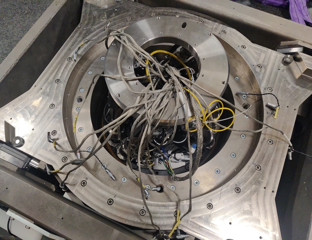
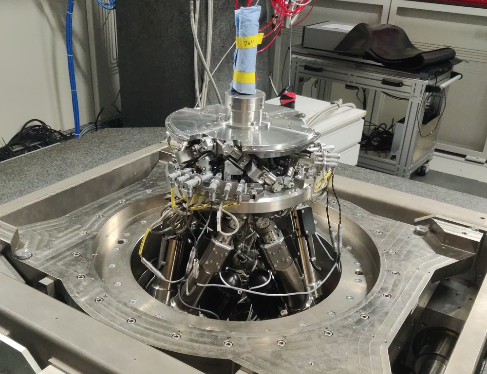
A first considered option was to use the "Spindle error analyzer" shown in Figure ref:fig:test_id31_lion. This system comprises 5 capacitive sensors which are facing two reference spheres. As the gap between the capacitive sensors and the spheres is very small¹, the risk of damaging the spheres and the capacitive sensors is high.

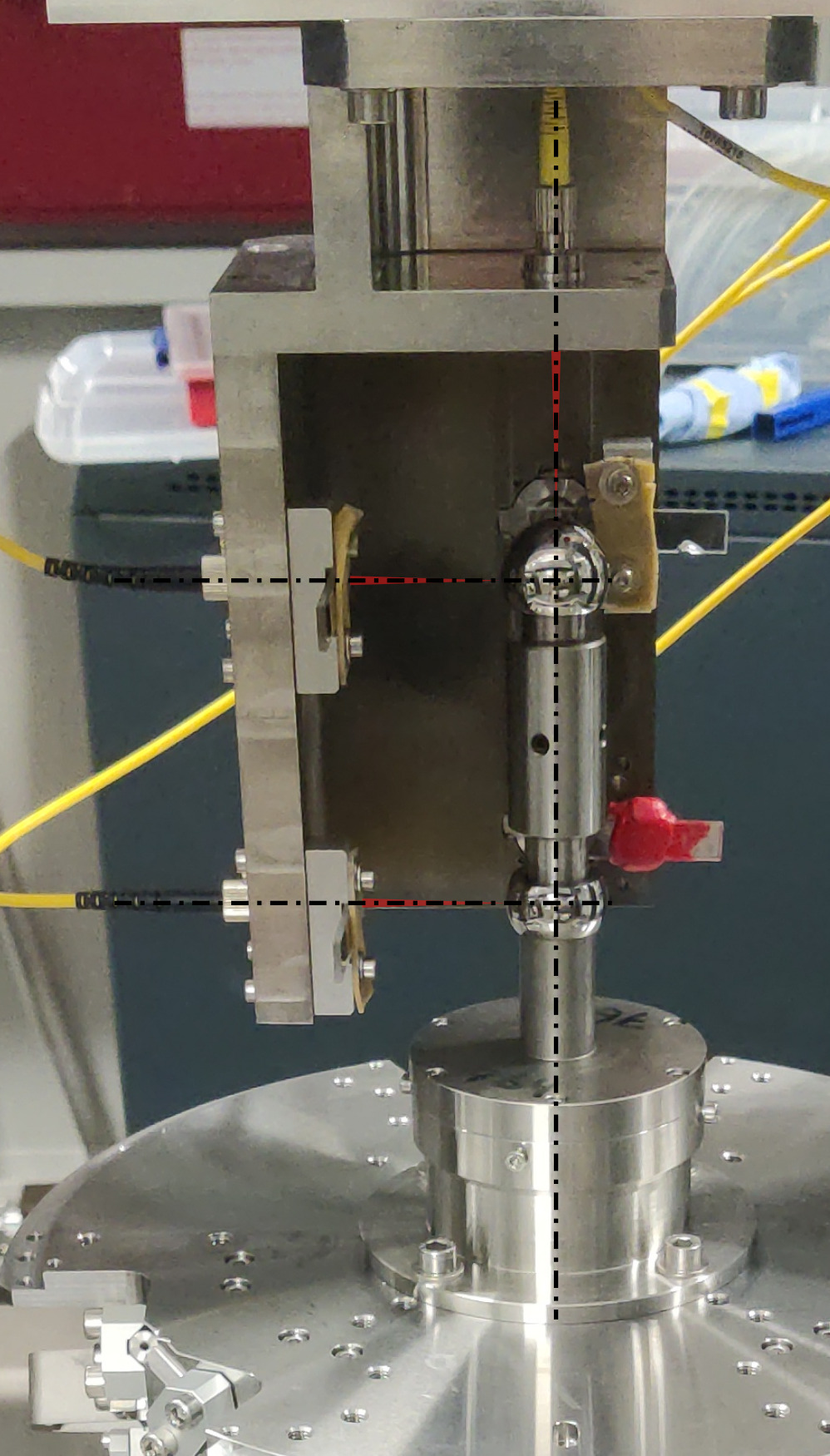
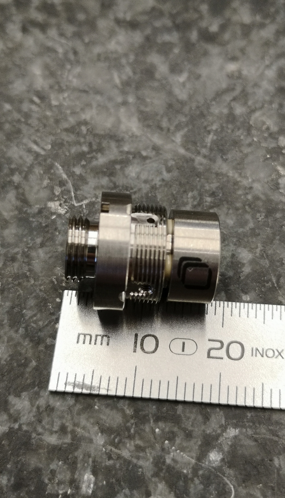
Instead of using capacitive sensors, 5 fibered interferometers were used in a similar way (Figure ref:fig:test_id31_interf). At the end of each fiber, a sensor head² (Figure ref:fig:test_id31_interf_head) is used, which consists of a lens precisely positioned with respect to the fiber's end. The lens is focusing the light on the surface of the sphere, such that it comes back to the fiber and produces an interference. This way, the gap between the sensor and the reference sphere is much larger (here around $40\,mm$), removing the risk of collision.

Nevertheless, the metrology system still has limited measurement range, as when the spheres are moving perpendicularly to the beam axis, the reflected light does not coincide with the incident light, and for some perpendicular displacement, the interference is too small to be detected.

Metrology Kinematics

<<ssec:test_id31_metrology_kinematics>>

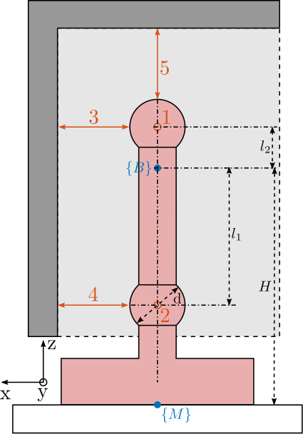
The developed short-stroke metrology system is schematically shown in Figure ref:fig:test_id31_metrology_kinematics. The point of interest is indicated by the blue frame $\{B\}$, which is located $H = 150\,mm$ above the nano-hexapod's top platform. The spheres have a diameter $d = 25.4\,mm$, and indicated dimensions are $l_1 = 60\,mm$ and $l_2 = 16.2\,mm$. In order to compute the pose of the $\{B\}$ frame with respect to the granite (i.e. with respect to the fixed interferometer heads), the measured small displacements $[d_1,\ d_2,\ d_3,\ d_4,\ d_5]$ by the interferometers are first written as a function of the small linear and angular motion of the $\{B\}$ frame $[D_x,\ D_y,\ D_z,\ R_x,\ R_y]$ eqref:eq:test_id31_metrology_kinematics.

\begin{equation}\label{eq:test_id31_metrology_kinematics} d_1 = D_y - l_2 R_x, \quad d_2 = D_y + l_1 R_x, \quad d_3 = -D_x - l_2 R_y, \quad d_4 = -D_x + l_1 R_y, \quad d_5 = -D_z

\end{equation}

\hfill

The top sphere is aligned with the rotation axis of the spindle using two probes.

The five equations eqref:eq:test_id31_metrology_kinematics can be written in a matrix form, and then inverted to have the pose of $\{B\}$ frame as a linear combination of the measured five distances by the interferometers eqref:eq:test_id31_metrology_kinematics_inverse.

\begin{equation}\label{eq:test_id31_metrology_kinematics_inverse}

\begin{bmatrix} D_x \\ D_y \\ D_z \\ R_x \\ R_y \end{bmatrix} = \begin{bmatrix} 0 & 1 & 0 & -l_2 & 0 \\ 0 & 1 & 0 & l_1 & 0 \\ -1 & 0 & 0 & 0 & -l_2 \\ -1 & 0 & 0 & 0 & l_1 \\ 0 & 0 & -1 & 0 & 0 \end{bmatrix}^{-1} \cdot \begin{bmatrix} d_1 \\ d_2 \\ d_3 \\ d_4 \\ d_5 \end{bmatrix}

\end{equation}

%% Geometrical parameters of the metrology system
H = 150e-3;
l1 = (150-48-42)*1e-3;
l2 = (76.2+48+42-150)*1e-3;

% Computation of the Transformation matrix
Hm = [ 0  1  0 -l2  0;
       0  1  0  l1  0;
      -1  0  0  0  -l2;
      -1  0  0  0   l1;
       0  0 -1  0   0];

Rough alignment of the reference spheres

<<ssec:test_id31_metrology_sphere_rought_alignment>>

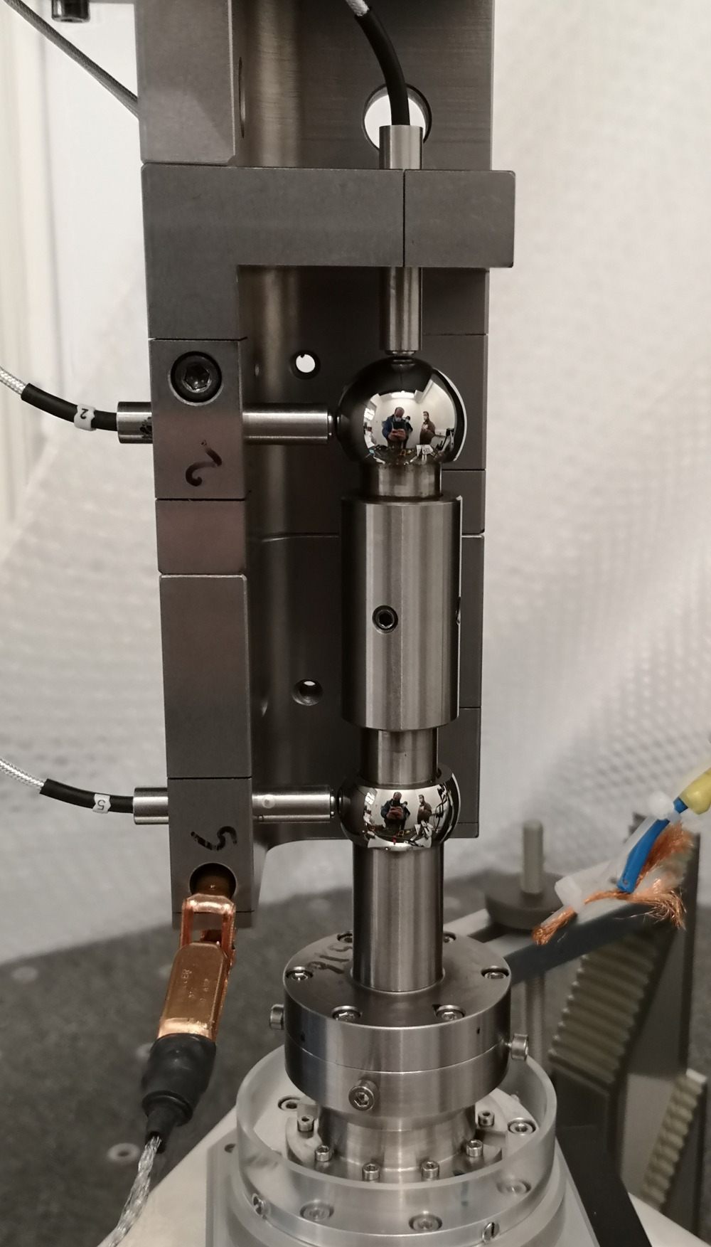
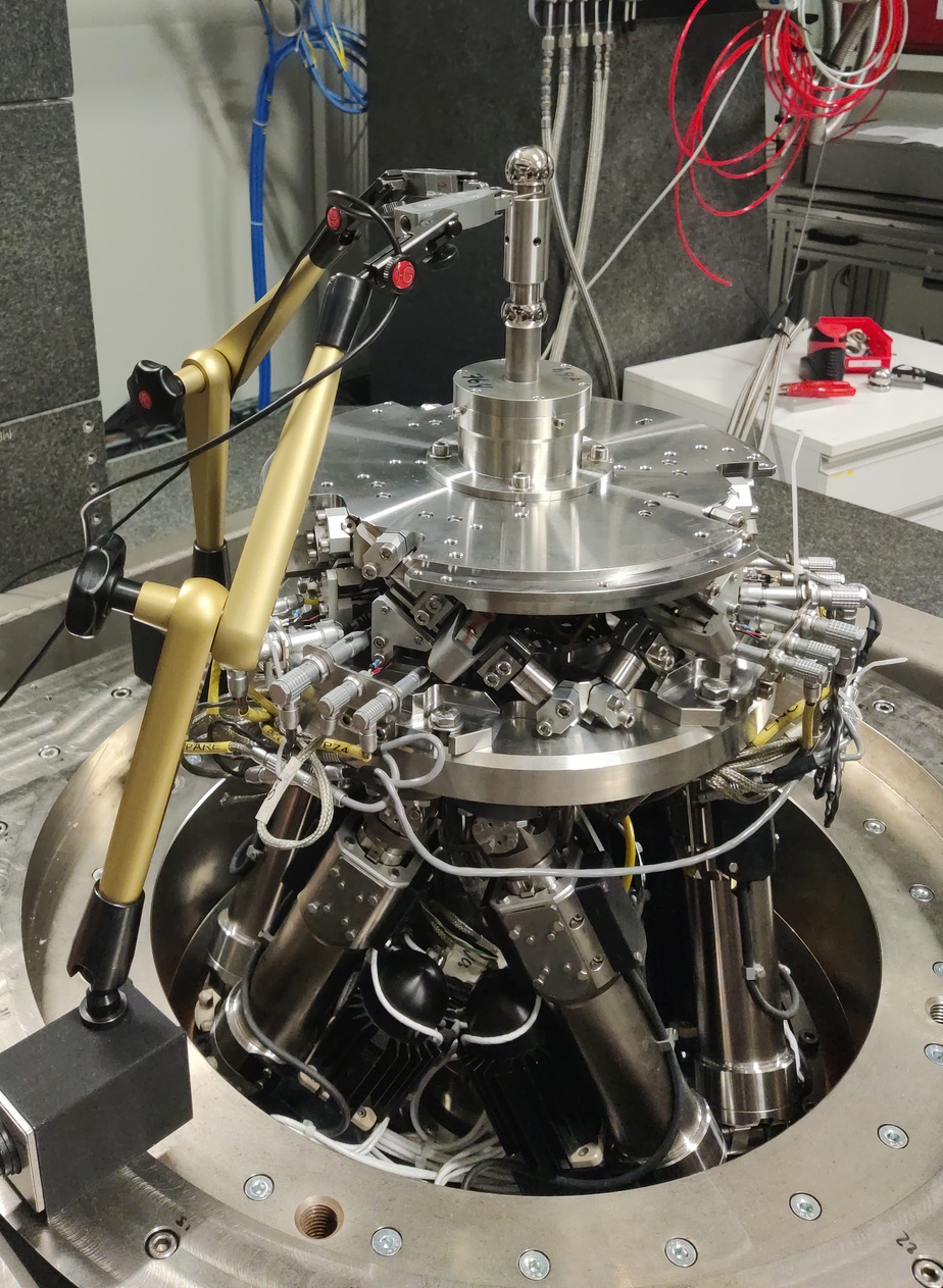
The two reference spheres are aligned with the rotation axis of the spindle. To do so, two measuring probes are used as shown in Figure ref:fig:align_top_sphere_comparators.

To not damage the sensitive sphere surface, the probes are instead positioned on the cylinder on which the sphere is mounted. First, the probes are fixed to the bottom (fixed) cylinder to align its axis with the spindle axis. Then, the probes are fixed to the top (adjustable) cylinder, and the same alignment is performed.

With this setup, the precision of the alignment of both sphere better with the spindle axis is expected to limited to $\approx 10\,\mu m$. This is probably limited due to the poor coaxiality between the cylinders and the spheres. However, the alignment precision should be enough to stay in the acceptance of the interferometers.

Tip-Tilt adjustment of the interferometers

<<ssec:test_id31_metrology_alignment>>

The short stroke metrology system is placed on top of the main granite using a gantry made of granite blocs to have good vibration and thermal stability (Figure ref:fig:short_stroke_metrology_overview).

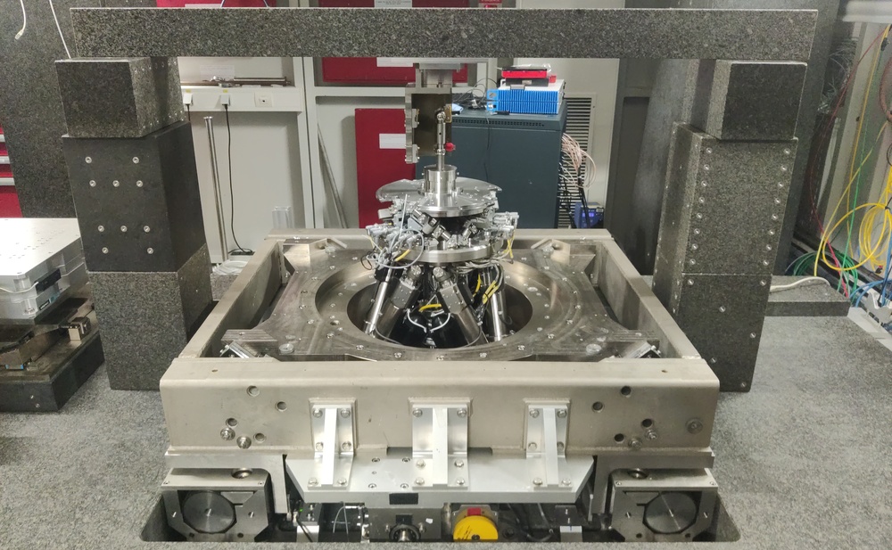
The interferometers need to be aligned with respect to the two reference spheres to approach as much as possible the ideal case shown in Figure ref:fig:test_id31_metrology_kinematics. The vertical position of the spheres is adjusted using the micro-hexapod to match the height of the interferometers. Then, the horizontal position of the gantry is adjusted such that the coupling efficiency (i.e. the intensity of the light reflected back in the fiber) of the top interferometer is maximized. This is equivalent as to optimize the perpendicularity between the interferometer beam and the sphere surface (i.e. the concentricity between the beam and the sphere center).

The lateral sensor heads (i.e. all except the top one), which are each fixed to a custom tip-tilt adjustment mechanism, are individually oriented such that the coupling efficient is maximized.

Fine Alignment of reference spheres using interferometers

<<ssec:test_id31_metrology_sphere_fine_alignment>>

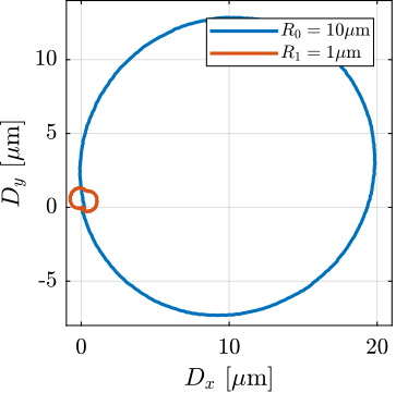
Thanks to the good alignment of the two reference spheres with the spindle axis and to the fine adjustment of the interferometers orientations, the interferometer measurement is made possible during complete spindle rotation. This metrology and therefore be used to better align the axis defined by the two spheres' center with the spindle axis.

The alignment process is made by few iterations. First, the spindle is scanned and the alignment errors are recorded. From the errors, the motion of the micro-hexapod to better align the spheres is determined and the micro-hexapod is moved. Then, the spindle is scanned again, and the new alignment errors are recorded.

This iterative process is first perform for angular errors (Figure ref:fig:test_id31_metrology_align_rx_ry) and then for lateral errors (Figure ref:fig:test_id31_metrology_align_dx_dy). Remaining error after alignment is in the order of $\pm5\,\mu\text{rad}$ for angular errors, $\pm 1\,\mu m$ laterally and less than $0.1\,\mu m$ vertically.

%% Angular alignment
% Load Data
data_it0 = h5scan(data_dir, 'alignment', 'h1rx_h1ry', 1);
data_it1 = h5scan(data_dir, 'alignment', 'h1rx_h1ry_0002', 3);
data_it2 = h5scan(data_dir, 'alignment', 'h1rx_h1ry_0002', 5);

% Offset wrong points
i_it0 = find(abs(data_it0.Rx_int_filtered(2:end)-data_it0.Rx_int_filtered(1:end-1))>1e-5);
data_it0.Rx_int_filtered(i_it0+1:end) = data_it0.Rx_int_filtered(i_it0+1:end) + data_it0.Rx_int_filtered(i_it0) - data_it0.Rx_int_filtered(i_it0+1);
i_it1 = find(abs(data_it1.Rx_int_filtered(2:end)-data_it1.Rx_int_filtered(1:end-1))>1e-5);
data_it1.Rx_int_filtered(i_it1+1:end) = data_it1.Rx_int_filtered(i_it1+1:end) + data_it1.Rx_int_filtered(i_it1) - data_it1.Rx_int_filtered(i_it1+1);
i_it2 = find(abs(data_it2.Rx_int_filtered(2:end)-data_it2.Rx_int_filtered(1:end-1))>1e-5);
data_it2.Rx_int_filtered(i_it2+1:end) = data_it2.Rx_int_filtered(i_it2+1:end) + data_it2.Rx_int_filtered(i_it2) - data_it2.Rx_int_filtered(i_it2+1);

% Compute circle fit and get radius
[~, ~, R_it0, ~] = circlefit(1e6*data_it0.Rx_int_filtered, 1e6*data_it0.Ry_int_filtered);
[~, ~, R_it1, ~] = circlefit(1e6*data_it1.Rx_int_filtered, 1e6*data_it1.Ry_int_filtered);
[~, ~, R_it2, ~] = circlefit(1e6*data_it2.Rx_int_filtered, 1e6*data_it2.Ry_int_filtered);

%% Eccentricity alignment
% Load Data
data_it0 = h5scan(data_dir, 'alignment', 'h1rx_h1ry_0002', 5);
data_it1 = h5scan(data_dir, 'alignment', 'h1dx_h1dy', 1);

% Offset wrong points
i_it0 = find(abs(data_it0.Dy_int_filtered(2:end)-data_it0.Dy_int_filtered(1:end-1))>1e-5);
data_it0.Dy_int_filtered(i_it0+1:end) = data_it0.Dy_int_filtered(i_it0+1:end) + data_it0.Dy_int_filtered(i_it0) - data_it0.Dy_int_filtered(i_it0+1);

% Compute circle fit and get radius
[~, ~, R_it0, ~] = circlefit(1e6*data_it0.Dx_int_filtered, 1e6*data_it0.Dy_int_filtered);
[~, ~, R_it1, ~] = circlefit(1e6*data_it1.Dx_int_filtered, 1e6*data_it1.Dy_int_filtered);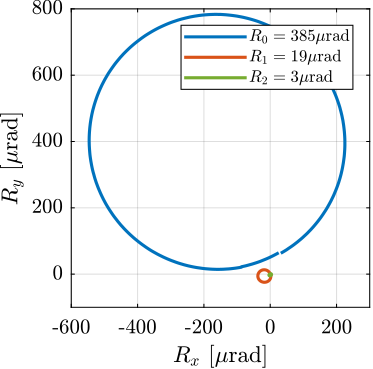

Estimated measurement volume

<<ssec:test_id31_metrology_acceptance>>

Because the interferometers are pointing to spheres and not flat surfaces, the lateral acceptance is limited. In order to estimate the metrology acceptance, the micro-hexapod is used to perform three accurate scans of $\pm 1\,mm$, respectively along the the $x$, $y$ and $z$ axes. During these scans, the 5 interferometers are recorded, and the ranges in which each interferometer has enough coupling efficiency for measurement are estimated. Results are summarized in Table ref:tab:test_id31_metrology_acceptance. The obtained lateral acceptance for pure displacements in any direction is estimated to be around $+/-0.5\,mm$, which is enough for the current application as it is well above the micro-station errors to be actively corrected.

%% Estimated acceptance of the metrology
% This is estimated by moving the spheres using the micro-hexapod

% Dx
data_dx = h5scan(data_dir, 'metrology_acceptance_new_align', 'dx', 1);

dx_acceptance = zeros(5,1);

for i = [1:size(dx_acceptance, 1)]
    % Find range in which the interferometers are measuring displacement
    dx_di = diff(data_dx.(sprintf('d%i', i))) == 0;
    if sum(dx_di) > 0
        dx_acceptance(i) = data_dx.h1tx(find(dx_di(501:end), 1) + 500) - ...
                           data_dx.h1tx(find(flip(dx_di(1:500)), 1));
    else
        dx_acceptance(i) = data_dx.h1tx(end) - data_dx.h1tx(1);
    end
end

% Dy
data_dy = h5scan(data_dir, 'metrology_acceptance_new_align', 'dy', 1);

dy_acceptance = zeros(5,1);

for i = [1:size(dy_acceptance, 1)]
    % Find range in which the interferometers are measuring displacement
    dy_di = diff(data_dy.(sprintf('d%i', i))) == 0;
    if sum(dy_di) > 0
        dy_acceptance(i) = data_dy.h1ty(find(dy_di(501:end), 1) + 500) - ...
                           data_dy.h1ty(find(flip(dy_di(1:500)), 1));
    else
        dy_acceptance(i) = data_dy.h1ty(end) - data_dy.h1ty(1);
    end
end

% Dz
data_dz = h5scan(data_dir, 'metrology_acceptance_new_align', 'dz', 1);

dz_acceptance = zeros(5,1);

for i = [1:size(dz_acceptance, 1)]
    % Find range in which the interferometers are measuring displacement
    dz_di = diff(data_dz.(sprintf('d%i', i))) == 0;
    if sum(dz_di) > 0
        dz_acceptance(i) = data_dz.h1tz(find(dz_di(501:end), 1) + 500) - ...
                           data_dz.h1tz(find(flip(dz_di(1:500)), 1));
    else
        dz_acceptance(i) = data_dz.h1tz(end) - data_dz.h1tz(1);
    end
end

	$D_x$	$D_y$	$D_z$
$d_1$ (y)	$1.0\,mm$	$>2\,mm$	$1.35\,mm$
$d_2$ (y)	$0.8\,mm$	$>2\,mm$	$1.01\,mm$
$d_3$ (x)	$>2\,mm$	$1.06\,mm$	$1.38\,mm$
$d_4$ (x)	$>2\,mm$	$0.99\,mm$	$0.94\,mm$
$d_5$ (z)	$1.33\, mm$	$1.06\,mm$	$>2\,mm$

Estimated measurement errors

<<ssec:test_id31_metrology_errors>>

When using the NASS, the accuracy of the sample's positioning is linked to the accuracy of the external metrology. However, to validate the nano-hexapod with the associated instrumentation and control architecture, the accuracy of the metrology is not an issue. Only the bandwidth and noise characteristics of the external metrology are important. Yet, some elements effecting the accuracy of the metrology are discussed here.

First, the "metrology kinematics" (discussed in Section ref:ssec:test_id31_metrology_kinematics) is only approximate (i.e. valid for very small displacements). This can be seen when performing lateral $[D_x,\,D_y]$ scans using the micro-hexapod while recording the vertical interferometer (Figure ref:fig:test_id31_xy_map_sphere). As the interferometer is pointing to a sphere and not to a plane, lateral motion of the sphere is seen as a vertical motion by the top interferometer.

Then, the reference spheres have some deviations with respect to an ideal sphere. They are meant to be used with capacitive sensors which are integrating the shape errors over large surfaces. When using interferometers, the size of the "light spot" on the sphere surface is a circle with a diameter $\approx 50\,\mu m$, therefore the system is more sensitive to shape errors with small features.

As the interferometer light is travelling in air, the measured distance is sensitive to any variation in the refractive index of the air. Therefore, any variation of air temperature, pressure or humidity will induce measurement errors. For a measurement length of $40\,mm$, a temperature variation of $0.1\,{}^oC$ induces an errors in the distance measurement of $\approx 4\,nm$.

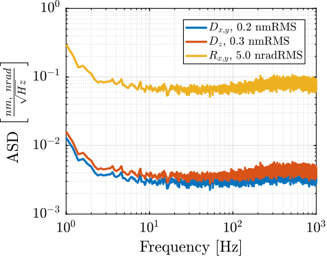
Finally, even in vacuum and in the absence of target motion, the interferometers are affected by noise cite:&watchi18_review_compac_inter. The effect of the noise on the translation and rotation measurements is estimated in Figure ref:fig:test_id31_interf_noise.

%% Interferometer noise estimation
data = load("test_id31_interf_noise.mat");

Ts = 1e-4;
Nfft = floor(5/Ts);
win = hanning(Nfft);
Noverlap = floor(Nfft/2);

[pxx_int, f] = pwelch(detrend(data.d, 0), win, Noverlap, Nfft, 1/Ts);

% Uncorrelated noise: square root of the sum of the squares
pxx_cart = pxx_int*sum(inv(Hm).^2, 2)';

rms_dxy = sqrt(trapz(f(f>1), pxx_cart((f>1),1))); % < 0.3 nm RMS
rms_dz  = sqrt(trapz(f(f>1), pxx_cart((f>1),3))); % < 0.3 nm RMS
rms_rxy = sqrt(trapz(f(f>1), pxx_cart((f>1),4))); % 5 nrad RMS

figure;
hold on;
plot(f, sqrt(pxx_cart(:,1)), 'DisplayName', sprintf('$D_{x,y}$, %.1f nmRMS', rms_dxy));
plot(f, sqrt(pxx_cart(:,3)), 'DisplayName', sprintf('$D_{z}$, %.1f nmRMS', rms_dz));
plot(f, sqrt(pxx_cart(:,4)), 'DisplayName', sprintf('$R_{x,y}$, %.1f nradRMS', rms_rxy));
set(gca, 'xscale', 'log'); set(gca, 'yscale', 'log');
xlabel('Frequency [Hz]'); ylabel('ASD $\left[\frac{nm,\ nrad}{\sqrt{Hz}}\right]$')
xlim([1, 1e3]); ylim([1e-3, 1]);
leg = legend('location', 'northeast', 'FontSize', 8, 'NumColumns', 1);
leg.ItemTokenSize(1) = 15;

%% X-Y scan with the micro-hexapod, and record of the vertical interferometer
data = h5scan(data_dir, 'metrology_acceptance', 'after_int_align_meshXY', 1);

x = 1e3*detrend(data.h1tx, 0); % [um]
y = 1e3*detrend(data.h1ty, 0); % [um]
z = 1e6*data.Dz_int_filtered - max(data.Dz_int_filtered); % [um]

mdl = scatteredInterpolant(x, y, z);
[xg, yg] = meshgrid(unique(x), unique(y));
zg = mdl(xg, yg);

% Fit a sphere to the data
[sphere_center,sphere_radius] = sphereFit(1e-3*[x, y, z]);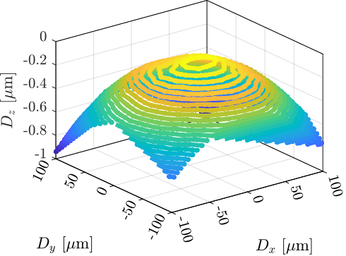

Identified Open Loop Plant

<<sec:test_id31_open_loop_plant>>

Introduction   ignore

• Force sensors: $\bm{V}_s = [V_{s1},\ V_{s2},\ V_{s3},\ V_{s4},\ V_{s5},\ V_{s6}]$
• Encoders: $\bm{d}_e = [d_{e1},\ d_{e2},\ d_{e3},\ d_{e4},\ d_{e5},\ d_{e6}]$
• Interferometers: $\bm{d} = [d_{1},\ d_{2},\ d_{3},\ d_{4},\ d_{5}]$
• Command signal: $\bm{u} = [u_1,\ u_2,\ u_3,\ u_4,\ u_5,\ u_6]$
• Voltage across the piezoelectric stack actuator: $\bm{V}_a = [V_{a1},\ V_{a2},\ V_{a3},\ V_{a4},\ V_{a5},\ V_{a6}]$
• Motion of the sample measured by external metrology: $\bm{y}_\mathcal{X} = [D_x,\,D_y,\,D_z,\,R_x,\,R_y,\,R_z]$

• Error of the sample measured by external metrology: $\bm{\epsilon\mathcal{X}} = [\epsilon_{D_x},\,\epsilon_{D_y},\,\epsilon_{D_z},\,\epsilon_{R_x},\,\epsilon_{R_y},\,\epsilon_{R_z}]$
• Error of the struts measured by external metrology: $\bm{\epsilon\mathcal{L}} = [\epsilon_{\mathcal{L}_1},\,\epsilon_{\mathcal{L}_2},\,\epsilon_{\mathcal{L}_3},\,\epsilon_{\mathcal{L}_4},\,\epsilon_{\mathcal{L}_5},\,\epsilon_{\mathcal{L}_6}]$
• Spindle angle setpoint (or encoder): $r_{R_z}$
• Translation stage setpoint: $r_{D_y}$
• Tilt stage setpoint: $r_{R_y}$

\begin{tikzpicture}
  % Blocs
  \node[block={2.0cm}{1.0cm}] (metrology) {Metrology};
  \node[block={2.0cm}{2.0cm}, below=0.1 of metrology, align=center] (nhexa) {Nano\\Hexapod};
  \node[block={4.0cm}{1.5cm}, below=0.1 of nhexa, align=center] (ustation) {Micro\\Station};

  \coordinate[] (inputVa)  at ($(nhexa.south west)!0.5!(nhexa.north west)$);
  \coordinate[] (outputVs) at ($(nhexa.south east)!0.3!(nhexa.north east)$);
  \coordinate[] (outputde) at ($(nhexa.south east)!0.7!(nhexa.north east)$);

  \coordinate[] (outputDy) at ($(ustation.south east)!0.1!(ustation.north east)$);
  \coordinate[] (outputRy) at ($(ustation.south east)!0.5!(ustation.north east)$);
  \coordinate[] (outputRz) at ($(ustation.south east)!0.9!(ustation.north east)$);

  \node[block={1.0cm}{1.0cm}, left=0.8 of inputVa] (pd200) {PD200};
  \node[block={1.0cm}{1.0cm}, right=0.8 of outputde] (Rz_kinematics) {$\bm{J}_{R_z}^{-1}$};
  \node[block={2.0cm}{2.0cm}, right=2.2 of ustation, align=center] (ustation_kinematics) {Compute\\Reference\\Position};
  \node[block={2.0cm}{2.0cm}, right=0.8 of ustation_kinematics, align=center] (compute_error) {Compute\\Error\\Position};
  \node[block={2.0cm}{2.0cm}, above=0.8 of compute_error, align=center] (compute_pos) {Compute\\Sample\\Position};
  \node[block={1.0cm}{1.0cm}, right=0.8 of compute_error] (hexa_jacobian) {$\bm{J}$};
  \node[block={1.0cm}{1.0cm}, right=0.8 of metrology] (metrology_kinematics) {$\bm{J}_d^{-1}$};

  \coordinate[] (inputMetrology) at ($(compute_error.north east)!0.3!(compute_error.north west)$);
  \coordinate[] (inputRz) at ($(compute_error.north east)!0.7!(compute_error.north west)$);

  \node[addb={+}{}{}{}{}, right=0.4 of Rz_kinematics] (addRz) {};
  \draw[->] (Rz_kinematics.east) -- (addRz.west);
  \draw[->] (outputRz-|addRz)node[branch]{} -- (addRz.south);

  \draw[->] (outputDy) node[above right]{$r_{D_y}$} -- (outputDy-|ustation_kinematics.west);
  \draw[->] (outputRy) node[above right]{$r_{R_y}$} -- (outputRy-|ustation_kinematics.west);
  \draw[->] (outputRz) node[above right]{$r_{R_z}$} -- (outputRz-|ustation_kinematics.west);

  \draw[->] (outputVs) -- ++(0.8, 0) node[above left]{$\bm{V}_s$};

  \draw[->] (metrology.east) -- (metrology_kinematics.west) node[above left]{$\bm{d}$};

  \draw[->] (metrology_kinematics.east)node[above right]{$[D_x,\,D_y,\,D_z,\,R_x,\,R_y]$} -- (compute_pos.west|-metrology_kinematics);
  \draw[->] (addRz.east)node[above right]{$R_z$} -- (compute_pos.west|-addRz);
  \draw[->] (compute_pos.south)node -- (compute_error.north)node[above right]{$\bm{y}_{\mathcal{X}}$};

  \draw[->] (outputde) -- (Rz_kinematics.west) node[above left]{$\bm{d}_{e}$};
  \draw[->] (ustation_kinematics.east) -- (compute_error.west) node[above left]{$\bm{r}_{\mathcal{X}}$};
  \draw[->] (compute_error.east) -- (hexa_jacobian.west) node[above left]{$\bm{\epsilon\mathcal{X}}$};
  \draw[->] (hexa_jacobian.east) -- ++(0.8, 0) node[above left]{$\bm{\epsilon\mathcal{L}}$};
  \draw[->] (pd200.east) -- (inputVa) node[above left]{$\bm{V}_a$};
  \draw[<-] (pd200.west) -- ++(-0.8, 0) node[above right]{$\bm{u}$};
\end{tikzpicture}

Schematic of the

First Open-Loop Plant Identification

<<ssec:test_id31_open_loop_plant_first_id>>

The plant dynamics is first identified for a fixed spindle angle (at $0\,\text{deg}$) and without any payload. The model dynamics is also identified in the same conditions.

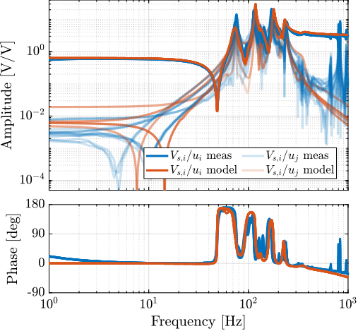
A first comparison between the model and the measured dynamics is done in Figure ref:fig:test_id31_first_id. A good match can be observed for the diagonal dynamics (except the high frequency modes which are not modeled). However, the coupling for the transfer function from command signals $\bm{u}$ to estimated strut motion from the external metrology $e\bm{\mathcal{L}}$ is larger than expected (Figure ref:fig:test_id31_first_id_int).

The experimental time delay estimated from the FRF (Figure ref:fig:test_id31_first_id_int) is larger than expected. After investigation, it was found that the additional delay was due to digital processing unit³ that was used to read the interferometers in the Speedgoat. This issue was later solved.

%% Identify the plant dynamics using the Simscape model

% Initialize each Simscape model elements
initializeGround();
initializeGranite();
initializeTy();
initializeRy();
initializeRz();
initializeMicroHexapod();
initializeNanoHexapod('flex_bot_type', '2dof', ...
                      'flex_top_type', '3dof', ...
                      'motion_sensor_type', 'plates', ...
                      'actuator_type', '2dof');
initializeSample('type', '0');

initializeSimscapeConfiguration('gravity', false);
initializeDisturbances('enable', false);
initializeLoggingConfiguration('log', 'none');
initializeController('type', 'open-loop');
initializeReferences();

% Input/Output definition
clear io; io_i = 1;
io(io_i) = linio([mdl, '/Controller'],     1, 'openinput');             io_i = io_i + 1; % Actuator Inputs [V]
io(io_i) = linio([mdl, '/Micro-Station'],  3, 'openoutput', [], 'Vs');  io_i = io_i + 1; % Force Sensors voltages [V]
io(io_i) = linio([mdl, '/Tracking Error'], 1, 'openoutput', [], 'EdL'); io_i = io_i + 1; % Position Errors [m]

% With no payload
Gm = exp(-1e-4*s)*linearize(mdl, io);
Gm.InputName  = {'u1', 'u2', 'u3', 'u4', 'u5', 'u6'};
Gm.OutputName = {'Vs1', 'Vs2', 'Vs3', 'Vs4', 'Vs5', 'Vs6', ...
                 'eL1', 'eL2', 'eL3', 'eL4', 'eL5', 'eL6'};

%% Identify the plant from experimental data

% Load identification data
data = load('2023-08-08_16-17_ol_plant_m0_Wz0.mat');

% Frequency analysis parameters
Ts = 1e-4; % Sampling Time [s]
Nfft = floor(2.0/Ts);
win = hanning(Nfft);
Noverlap = floor(Nfft/2);
[~, f] = tfestimate(data.uL1.id_plant, data.uL1.e_L1, win, Noverlap, Nfft, 1/Ts);

G_iff = zeros(length(f), 6, 6); % Force sensor outputs
G_int = zeros(length(f), 6, 6); % Estimated strut errors
for i_strut = 1:6
    Vs = [data.(sprintf("uL%i", i_strut)).Vs1 ; data.(sprintf("uL%i", i_strut)).Vs2 ; data.(sprintf("uL%i", i_strut)).Vs3 ; data.(sprintf("uL%i", i_strut)).Vs4 ; data.(sprintf("uL%i", i_strut)).Vs5 ; data.(sprintf("uL%i", i_strut)).Vs6]';
    eL = [data.(sprintf("uL%i", i_strut)).e_L1 ; data.(sprintf("uL%i", i_strut)).e_L2 ; data.(sprintf("uL%i", i_strut)).e_L3 ; data.(sprintf("uL%i", i_strut)).e_L4 ; data.(sprintf("uL%i", i_strut)).e_L5 ; data.(sprintf("uL%i", i_strut)).e_L6]';
    dL = [data.(sprintf("uL%i", i_strut)).dL1 ; data.(sprintf("uL%i", i_strut)).dL2 ; data.(sprintf("uL%i", i_strut)).dL3 ; data.(sprintf("uL%i", i_strut)).dL4 ; data.(sprintf("uL%i", i_strut)).dL5 ; data.(sprintf("uL%i", i_strut)).dL6]';

    G_iff(:,:,i_strut) = tfestimate(data.(sprintf("uL%i", i_strut)).id_plant, Vs, win, Noverlap, Nfft, 1/Ts);
    G_int(:,:,i_strut) = tfestimate(data.(sprintf("uL%i", i_strut)).id_plant, eL, win, Noverlap, Nfft, 1/Ts);
end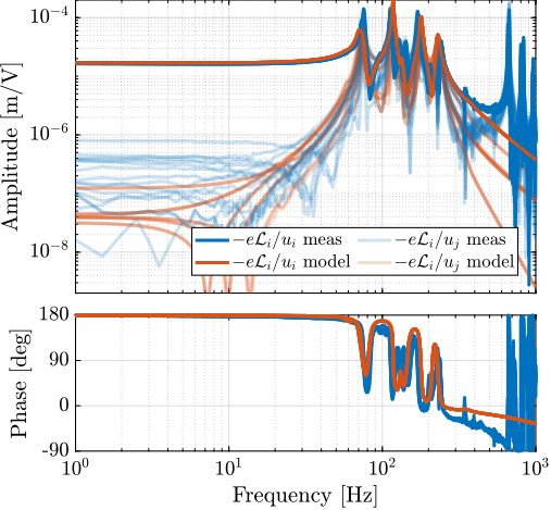

Better Angular Alignment

<<ssec:test_id31_open_loop_plant_rz_alignment>>

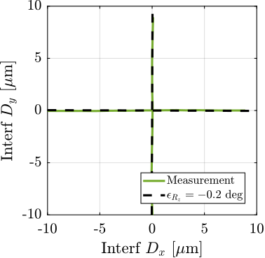
One possible explanation of the increased coupling observed in Figure ref:fig:test_id31_first_id_int is the poor alignment between the external metrology axes (i.e. the interferometer supports) and the nano-hexapod axes. To estimate this alignment, a decentralized low-bandwidth feedback controller based on the nano-hexapod encoders is implemented. This allowed to perform two straight movements of the nano-hexapod along the $x$ and $y$ axes in the frame of the nano-hexapod. During these two movements, the external metrology measurement is recorded and shown in Figure ref:fig:test_id31_Rz_align_error. It was found that there is a misalignment of 2.7 degrees (rotation along the vertical axis) between the interferometer axes and nano-hexapod axes. This was corrected by adding an offset to the spindle angle. To check that the alignment has improved, the same movement was performed using the nano-hexapod while recording the signal of the external metrology. Results shown in Figure ref:fig:test_id31_Rz_align_correct are indeed indicating much better alignment.

%% Load Data
data_1_dx = h5scan(data_dir, 'align_int_enc_Rz', 'tx_first_scan', 2);
data_1_dy = h5scan(data_dir, 'align_int_enc_Rz', 'tx_first_scan', 3);
data_2_dx = h5scan(data_dir, 'align_int_enc_Rz', 'verif-after-correct-offset', 1);
data_2_dy = h5scan(data_dir, 'align_int_enc_Rz', 'verif-after-correct-offset', 2);

% Estimation of Rz misalignment
p1 = polyfit(data_1_dx.Dx_int_filtered, data_1_dx.Dy_int_filtered, 1);
p2 = polyfit(data_1_dy.Dx_int_filtered, data_1_dy.Dy_int_filtered, 1);

Rz_error = (atan(p1(1)) + atan(p2(1))-pi/2)/2; % ~3 degrees

%% Estimation of the Rz misalignment
figure;
hold on;
plot(1e6*data_1_dx.Dx_int_filtered, 1e6*data_1_dx.Dy_int_filtered, 'color', colors(2,:), 'DisplayName', 'Measurement')
plot(1e6*data_1_dy.Dx_int_filtered, 1e6*data_1_dy.Dy_int_filtered, 'color', colors(2,:), 'HandleVisibility', 'off')
plot( 1e6*[-10:10]*cos(Rz_error), 1e6*[-10:10]*sin(Rz_error), 'k--', 'DisplayName', sprintf('$\\epsilon_{R_z} = %.1f$ deg', Rz_error*180/pi))
plot(-1e6*[-10:10]*sin(Rz_error), 1e6*[-10:10]*cos(Rz_error), 'k--', 'HandleVisibility', 'off')
hold off;
xlabel('Interf $D_x$ [$\mu$m]');
ylabel('Interf $D_y$ [$\mu$m]');
axis equal
xlim([-10, 10]); ylim([-10, 10]);
xticks([-10:5:10]); yticks([-10:5:10]);
leg = legend('location', 'southeast', 'FontSize', 8, 'NumColumns', 1);
leg.ItemTokenSize(1) = 15;

% Estimation of Rz misalignment after correcting the Rz angle
p1 = polyfit(data_2_dx.Dx_int_filtered, data_2_dx.Dy_int_filtered, 1);
p2 = polyfit(data_2_dy.Dx_int_filtered, data_2_dy.Dy_int_filtered, 1);

Rz_error = (atan(p1(1)) + atan(p2(1))-pi/2)/2; % ~0.2 degrees

%% Estimation of the Rz misalignment after correcting the Rz offset
figure;
hold on;
plot(1e6*data_2_dx.Dx_int_filtered, 1e6*data_2_dx.Dy_int_filtered, 'color', colors(5,:), 'DisplayName', 'Measurement')
plot(1e6*data_2_dy.Dx_int_filtered, 1e6*data_2_dy.Dy_int_filtered, 'color', colors(5,:), 'HandleVisibility', 'off')
plot( 1e6*[-10:10]*cos(Rz_error), 1e6*[-10:10]*sin(Rz_error), 'k--', 'DisplayName', sprintf('$\\epsilon_{R_z} = %.1f$ deg', Rz_error*180/pi))
plot(-1e6*[-10:10]*sin(Rz_error), 1e6*[-10:10]*cos(Rz_error), 'k--', 'HandleVisibility', 'off')
hold off;
xlabel('Interf $D_x$ [$\mu$m]');
ylabel('Interf $D_y$ [$\mu$m]');
axis equal
xlim([-10, 10]); ylim([-10, 10]);
xticks([-10:5:10]); yticks([-10:5:10]);
leg = legend('location', 'southeast', 'FontSize', 8, 'NumColumns', 1);
leg.ItemTokenSize(1) = 15;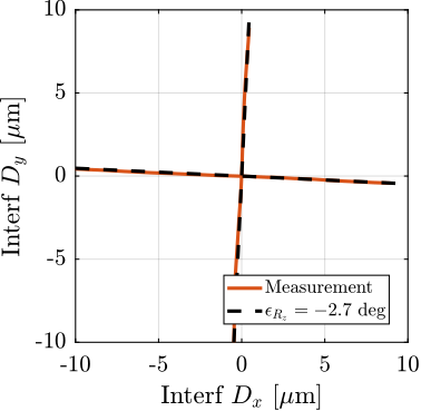

Open-Loop Identification after alignment

<<ssec:test_id31_open_loop_plant_after_alignment>>

The plant dynamics is identified after the fine alignment and is compared with the model dynamics in Figure ref:fig:test_id31_first_id_int_better_rz_align. Compared to the initial identification shown in Figure ref:fig:test_id31_first_id_int, the obtained coupling has decreased and is now close to the coupling obtained with the multi-body model. At low frequency (below $10\,\text{Hz}$) all the off-diagonal elements have an amplitude $\approx 100$ times lower compared to the diagonal elements, indicating that a low bandwidth feedback controller can be implemented in a decentralized way (i.e. $6$ SISO controllers).

%% Identification of the plant after Rz alignment
data_align = load('2023-08-17_17-37_ol_plant_m0_Wz0_new_Rz_align.mat');

G_int_align = zeros(length(f), 6, 6);
for i_strut = 1:6
    eL = [data_align.(sprintf("uL%i", i_strut)).e_L1 ; data_align.(sprintf("uL%i", i_strut)).e_L2 ; data_align.(sprintf("uL%i", i_strut)).e_L3 ; data_align.(sprintf("uL%i", i_strut)).e_L4 ; data_align.(sprintf("uL%i", i_strut)).e_L5 ; data_align.(sprintf("uL%i", i_strut)).e_L6]';

    G_int_align(:,:,i_strut) = tfestimate(data_align.(sprintf("uL%i", i_strut)).id_plant, eL, win, Noverlap, Nfft, 1/Ts);
end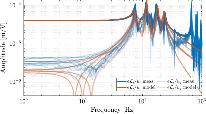

Decrease of the coupling with better Rz alignment

Effect of Payload Mass

<<ssec:test_id31_open_loop_plant_mass>>

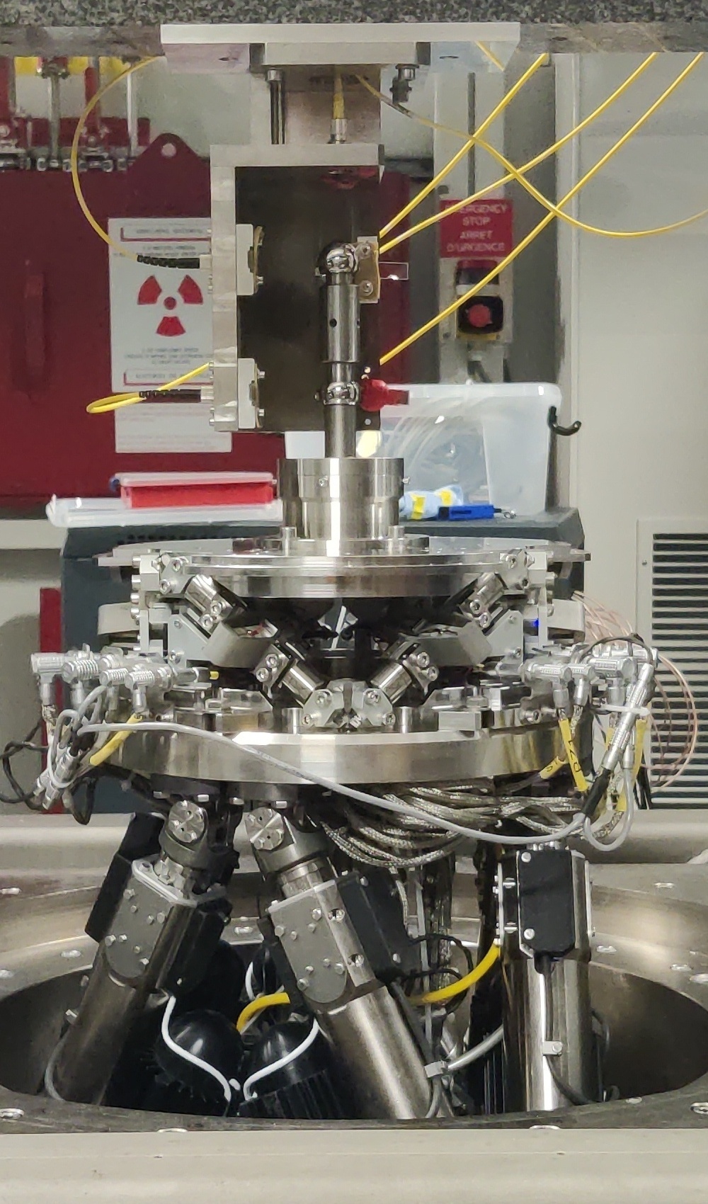
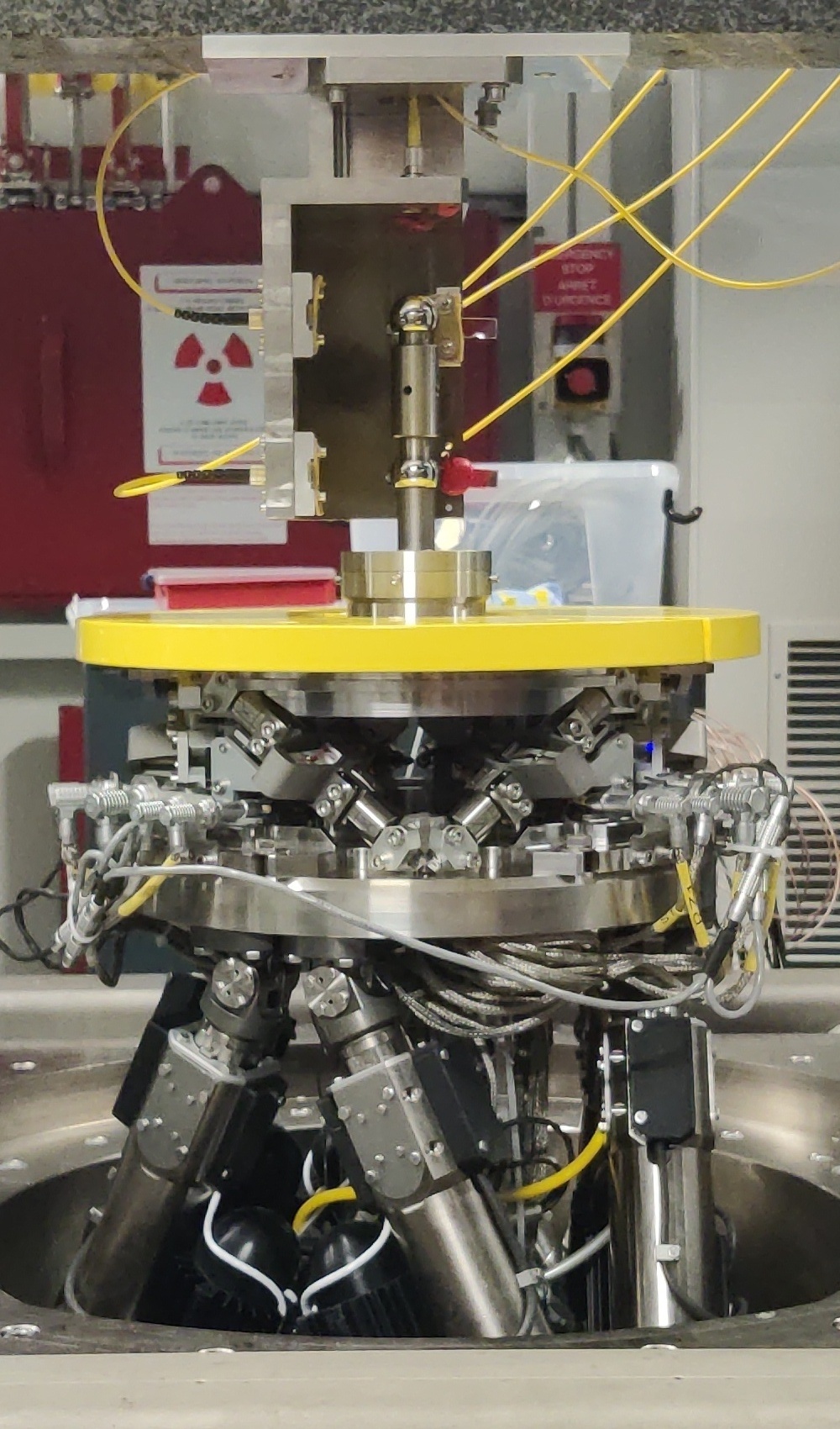
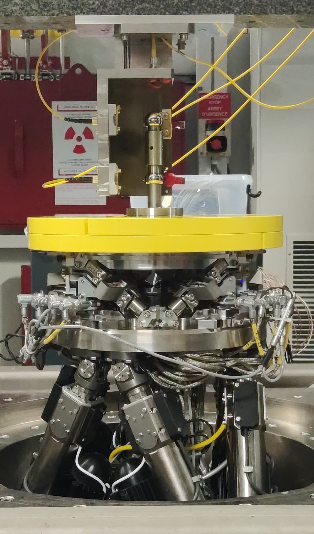
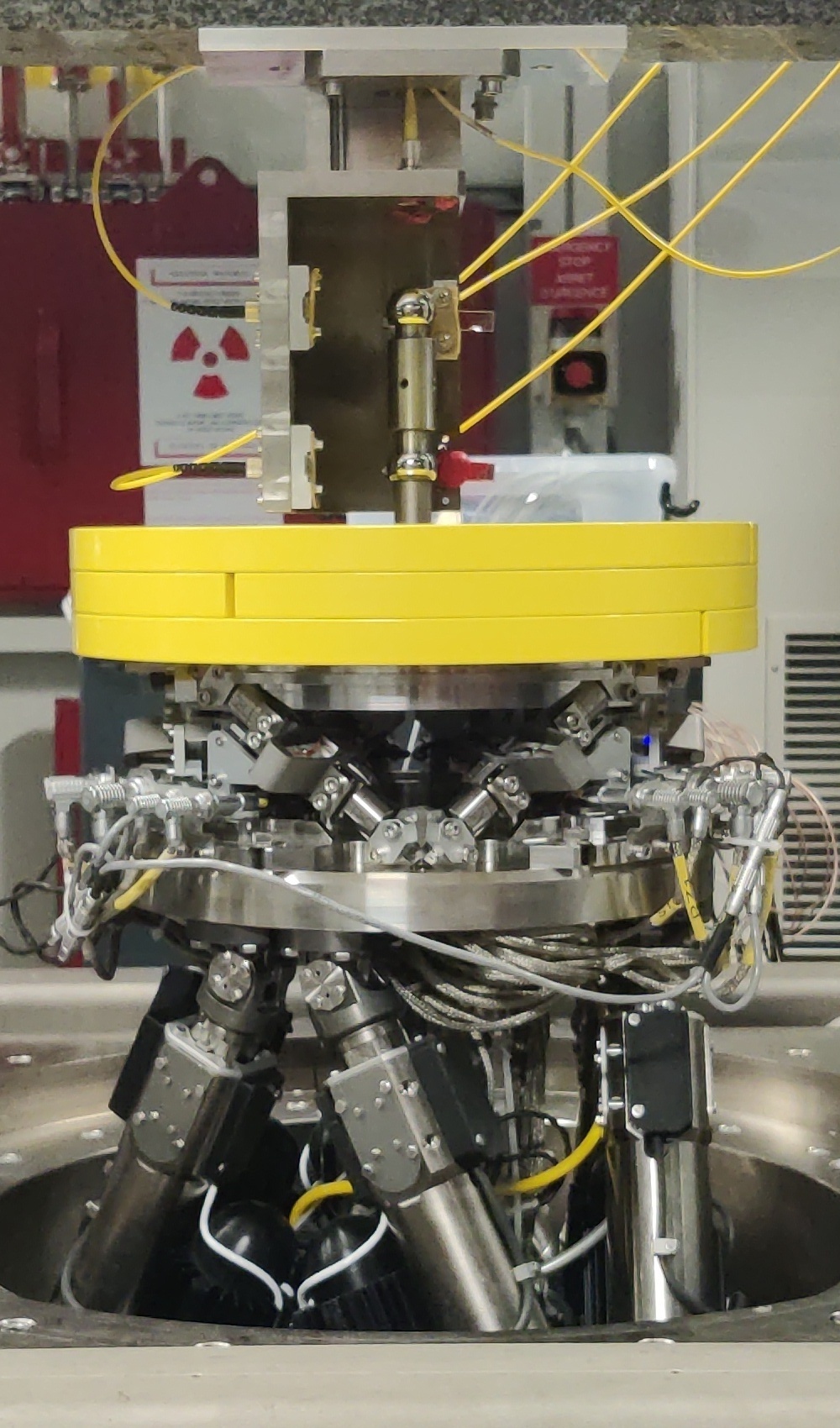
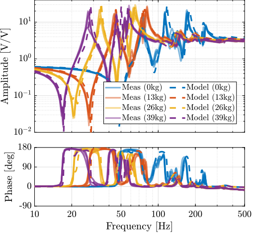
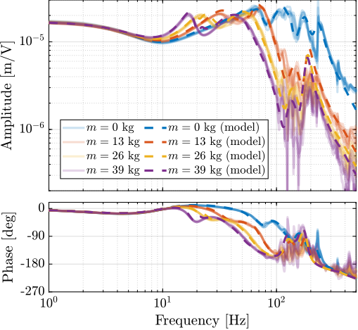
The system dynamics was identified with four payload conditions that are shown in Figure ref:fig:test_id31_picture_masses. The obtained direct terms are compared with the model dynamics in Figure ref:fig:test_nhexa_comp_simscape_diag_masses.

It is interesting to note that the anti-resonances in the force sensor plant are now appearing as minimum-phase, as the model predicts (Figure ref:fig:test_id31_comp_simscape_iff_diag_masses).

%% Identify the plant from experimental data - All payloads

% Load identification data
data_m0_Wz0 = load('2023-08-08_16-17_ol_plant_m0_Wz0.mat');
data_m1_Wz0 = load('2023-08-08_18-57_ol_plant_m1_Wz0.mat');
data_m2_Wz0 = load('2023-08-08_17-12_ol_plant_m2_Wz0.mat');
data_m3_Wz0 = load('2023-08-08_18-20_ol_plant_m3_Wz0.mat');

% Sampling Time [s]
Ts = 1e-4;

% Hannning Windows
Nfft = floor(2.0/Ts);
win = hanning(Nfft);
Noverlap = floor(Nfft/2);

% And we get the frequency vector
[~, f] = tfestimate(data_m0_Wz0.uL1.id_plant, data_m0_Wz0.uL1.e_L1, win, Noverlap, Nfft, 1/Ts);

% No payload
G_iff_m0_Wz0 = zeros(length(f), 6, 6);
for i_strut = 1:6
    eL = [data_m0_Wz0.(sprintf("uL%i", i_strut)).Vs1 ; data_m0_Wz0.(sprintf("uL%i", i_strut)).Vs2 ; data_m0_Wz0.(sprintf("uL%i", i_strut)).Vs3 ; data_m0_Wz0.(sprintf("uL%i", i_strut)).Vs4 ; data_m0_Wz0.(sprintf("uL%i", i_strut)).Vs5 ; data_m0_Wz0.(sprintf("uL%i", i_strut)).Vs6]';

    G_iff_m0_Wz0(:,:,i_strut) = tfestimate(data_m0_Wz0.(sprintf("uL%i", i_strut)).id_plant, eL, win, Noverlap, Nfft, 1/Ts);
end

G_int_m0_Wz0 = zeros(length(f), 6, 6);
for i_strut = 1:6
    eL = [data_m0_Wz0.(sprintf("uL%i", i_strut)).e_L1 ; data_m0_Wz0.(sprintf("uL%i", i_strut)).e_L2 ; data_m0_Wz0.(sprintf("uL%i", i_strut)).e_L3 ; data_m0_Wz0.(sprintf("uL%i", i_strut)).e_L4 ; data_m0_Wz0.(sprintf("uL%i", i_strut)).e_L5 ; data_m0_Wz0.(sprintf("uL%i", i_strut)).e_L6]';

    G_int_m0_Wz0(:,:,i_strut) = tfestimate(data_m0_Wz0.(sprintf("uL%i", i_strut)).id_plant, eL, win, Noverlap, Nfft, 1/Ts);
end

% 1 "payload layer"
G_iff_m1_Wz0 = zeros(length(f), 6, 6);
for i_strut = 1:6
    eL = [data_m1_Wz0.(sprintf("uL%i", i_strut)).Vs1 ; data_m1_Wz0.(sprintf("uL%i", i_strut)).Vs2 ; data_m1_Wz0.(sprintf("uL%i", i_strut)).Vs3 ; data_m1_Wz0.(sprintf("uL%i", i_strut)).Vs4 ; data_m1_Wz0.(sprintf("uL%i", i_strut)).Vs5 ; data_m1_Wz0.(sprintf("uL%i", i_strut)).Vs6]';

    G_iff_m1_Wz0(:,:,i_strut) = tfestimate(data_m1_Wz0.(sprintf("uL%i", i_strut)).id_plant, eL, win, Noverlap, Nfft, 1/Ts);
end

G_int_m1_Wz0 = zeros(length(f), 6, 6);
for i_strut = 1:6
    eL = [data_m1_Wz0.(sprintf("uL%i", i_strut)).e_L1 ; data_m1_Wz0.(sprintf("uL%i", i_strut)).e_L2 ; data_m1_Wz0.(sprintf("uL%i", i_strut)).e_L3 ; data_m1_Wz0.(sprintf("uL%i", i_strut)).e_L4 ; data_m1_Wz0.(sprintf("uL%i", i_strut)).e_L5 ; data_m1_Wz0.(sprintf("uL%i", i_strut)).e_L6]';

    G_int_m1_Wz0(:,:,i_strut) = tfestimate(data_m1_Wz0.(sprintf("uL%i", i_strut)).id_plant, eL, win, Noverlap, Nfft, 1/Ts);
end

% 2 "payload layers"
G_iff_m2_Wz0 = zeros(length(f), 6, 6);
for i_strut = 1:6
    eL = [data_m2_Wz0.(sprintf("uL%i", i_strut)).Vs1 ; data_m2_Wz0.(sprintf("uL%i", i_strut)).Vs2 ; data_m2_Wz0.(sprintf("uL%i", i_strut)).Vs3 ; data_m2_Wz0.(sprintf("uL%i", i_strut)).Vs4 ; data_m2_Wz0.(sprintf("uL%i", i_strut)).Vs5 ; data_m2_Wz0.(sprintf("uL%i", i_strut)).Vs6]';

    G_iff_m2_Wz0(:,:,i_strut) = tfestimate(data_m2_Wz0.(sprintf("uL%i", i_strut)).id_plant, eL, win, Noverlap, Nfft, 1/Ts);
end

G_int_m2_Wz0 = zeros(length(f), 6, 6);
for i_strut = 1:6
    eL = [data_m2_Wz0.(sprintf("uL%i", i_strut)).e_L1 ; data_m2_Wz0.(sprintf("uL%i", i_strut)).e_L2 ; data_m2_Wz0.(sprintf("uL%i", i_strut)).e_L3 ; data_m2_Wz0.(sprintf("uL%i", i_strut)).e_L4 ; data_m2_Wz0.(sprintf("uL%i", i_strut)).e_L5 ; data_m2_Wz0.(sprintf("uL%i", i_strut)).e_L6]';

    G_int_m2_Wz0(:,:,i_strut) = tfestimate(data_m2_Wz0.(sprintf("uL%i", i_strut)).id_plant, eL, win, Noverlap, Nfft, 1/Ts);
end

% 3 "payload layers"
G_iff_m3_Wz0 = zeros(length(f), 6, 6);
for i_strut = 1:6
    eL = [data_m3_Wz0.(sprintf("uL%i", i_strut)).Vs1 ; data_m3_Wz0.(sprintf("uL%i", i_strut)).Vs2 ; data_m3_Wz0.(sprintf("uL%i", i_strut)).Vs3 ; data_m3_Wz0.(sprintf("uL%i", i_strut)).Vs4 ; data_m3_Wz0.(sprintf("uL%i", i_strut)).Vs5 ; data_m3_Wz0.(sprintf("uL%i", i_strut)).Vs6]';

    G_iff_m3_Wz0(:,:,i_strut) = tfestimate(data_m3_Wz0.(sprintf("uL%i", i_strut)).id_plant, eL, win, Noverlap, Nfft, 1/Ts);
end

G_int_m3_Wz0 = zeros(length(f), 6, 6);
for i_strut = 1:6
    eL = [data_m3_Wz0.(sprintf("uL%i", i_strut)).e_L1 ; data_m3_Wz0.(sprintf("uL%i", i_strut)).e_L2 ; data_m3_Wz0.(sprintf("uL%i", i_strut)).e_L3 ; data_m3_Wz0.(sprintf("uL%i", i_strut)).e_L4 ; data_m3_Wz0.(sprintf("uL%i", i_strut)).e_L5 ; data_m3_Wz0.(sprintf("uL%i", i_strut)).e_L6]';

    G_int_m3_Wz0(:,:,i_strut) = tfestimate(data_m3_Wz0.(sprintf("uL%i", i_strut)).id_plant, eL, win, Noverlap, Nfft, 1/Ts);
end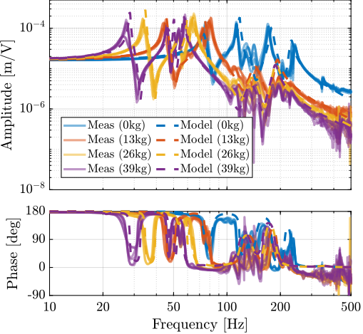

Effect of Spindle Rotation

<<ssec:test_id31_open_loop_plant_rotation>>

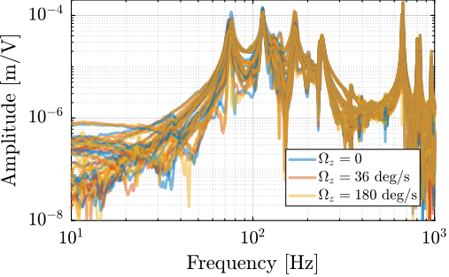
The dynamics was then identified while the Spindle was rotating at constant velocity. Three identification experiments were performed: no spindle rotation, spindle rotation at $36\,\text{deg}/s$ and at $180\,\text{deg}/s$.

The comparison of the obtained dynamics from command signal $u$ to estimated strut error $e\mathcal{L}$ is done in Figure ref:fig:test_id31_effect_rotation. Both direct terms (Figure ref:fig:test_id31_effect_rotation_direct) and coupling terms (Figure ref:fig:test_id31_effect_rotation_coupling) are unaffected by the rotation. The same can be observed for the dynamics from the command signal to the encoders and to the force sensors. This confirms that the rotation has no significant effect on the plant dynamics. This also indicates that the metrology kinematics is correct and is working in real time.

%% Identify the model dynamics with Spindle rotation
initializeSample('type', '0');
initializeReferences(...
    'Rz_type', 'rotating', ...
    'Rz_period', 360/36); % 36 deg/s, 6rpm
Gm_m0_Wz36 = linearize(mdl, io, 0.1);
Gm_m0_Wz36.InputName  = {'u1', 'u2', 'u3', 'u4', 'u5', 'u6'};
Gm_m0_Wz36.OutputName = {'Vs1', 'Vs2', 'Vs3', 'Vs4', 'Vs5', 'Vs6', ...
                         'eL1', 'eL2', 'eL3', 'eL4', 'eL5', 'eL6'};

initializeReferences(...
    'Rz_type', 'rotating', ...
    'Rz_period', 360/180); % 180 deg/s, 30rpm
Gm_m0_Wz180 = linearize(mdl, io, 0.1);
Gm_m0_Wz180.InputName  = {'u1', 'u2', 'u3', 'u4', 'u5', 'u6'};
Gm_m0_Wz180.OutputName = {'Vs1', 'Vs2', 'Vs3', 'Vs4', 'Vs5', 'Vs6', ...
                          'eL1', 'eL2', 'eL3', 'eL4', 'eL5', 'eL6'};

%% Identify the plant from experimental data - Effect of rotation

% Load identification data
data_m0_Wz36  = load('2023-08-08_16-28_ol_plant_m0_Wz36.mat');
data_m0_Wz180 = load('2023-08-08_16-45_ol_plant_m0_Wz180.mat');

% Spindle Rotation at 36 deg/s
G_iff_m0_Wz36 = zeros(length(f), 6, 6);
for i_strut = 1:6
    eL = [data_m0_Wz36.(sprintf("uL%i", i_strut)).Vs1 ; data_m0_Wz36.(sprintf("uL%i", i_strut)).Vs2 ; data_m0_Wz36.(sprintf("uL%i", i_strut)).Vs3 ; data_m0_Wz36.(sprintf("uL%i", i_strut)).Vs4 ; data_m0_Wz36.(sprintf("uL%i", i_strut)).Vs5 ; data_m0_Wz36.(sprintf("uL%i", i_strut)).Vs6]';

    G_iff_m0_Wz36(:,:,i_strut) = tfestimate(data_m0_Wz36.(sprintf("uL%i", i_strut)).id_plant, eL, win, Noverlap, Nfft, 1/Ts);
end

G_int_m0_Wz36 = zeros(length(f), 6, 6);
for i_strut = 1:6
    eL = [data_m0_Wz36.(sprintf("uL%i", i_strut)).e_L1 ; data_m0_Wz36.(sprintf("uL%i", i_strut)).e_L2 ; data_m0_Wz36.(sprintf("uL%i", i_strut)).e_L3 ; data_m0_Wz36.(sprintf("uL%i", i_strut)).e_L4 ; data_m0_Wz36.(sprintf("uL%i", i_strut)).e_L5 ; data_m0_Wz36.(sprintf("uL%i", i_strut)).e_L6]';

    G_int_m0_Wz36(:,:,i_strut) = tfestimate(data_m0_Wz36.(sprintf("uL%i", i_strut)).id_plant, eL, win, Noverlap, Nfft, 1/Ts);
end

% Spindle Rotation at 180 deg/s
G_iff_m0_Wz180 = zeros(length(f), 6, 6);
for i_strut = 1:6
    eL = [data_m0_Wz180.(sprintf("uL%i", i_strut)).Vs1 ; data_m0_Wz180.(sprintf("uL%i", i_strut)).Vs2 ; data_m0_Wz180.(sprintf("uL%i", i_strut)).Vs3 ; data_m0_Wz180.(sprintf("uL%i", i_strut)).Vs4 ; data_m0_Wz180.(sprintf("uL%i", i_strut)).Vs5 ; data_m0_Wz180.(sprintf("uL%i", i_strut)).Vs6]';

    G_iff_m0_Wz180(:,:,i_strut) = tfestimate(data_m0_Wz180.(sprintf("uL%i", i_strut)).id_plant, eL, win, Noverlap, Nfft, 1/Ts);
end

G_int_m0_Wz180 = zeros(length(f), 6, 6);
for i_strut = 1:6
    eL = [data_m0_Wz180.(sprintf("uL%i", i_strut)).e_L1 ; data_m0_Wz180.(sprintf("uL%i", i_strut)).e_L2 ; data_m0_Wz180.(sprintf("uL%i", i_strut)).e_L3 ; data_m0_Wz180.(sprintf("uL%i", i_strut)).e_L4 ; data_m0_Wz180.(sprintf("uL%i", i_strut)).e_L5 ; data_m0_Wz180.(sprintf("uL%i", i_strut)).e_L6]';

    G_int_m0_Wz180(:,:,i_strut) = tfestimate(data_m0_Wz180.(sprintf("uL%i", i_strut)).id_plant, eL, win, Noverlap, Nfft, 1/Ts);
end

% The identified dynamics are then saved for further use.
save('./mat/test_id31_simscape_open_loop_plants.mat', 'Gm_m0_Wz0', 'Gm_m0_Wz36', 'Gm_m0_Wz180', 'Gm_m1_Wz0', 'Gm_m2_Wz0', 'Gm_m3_Wz0');
save('./mat/test_id31_identified_open_loop_plants.mat', 'G_int_m0_Wz0', 'G_int_m0_Wz36', 'G_int_m0_Wz180', 'G_int_m1_Wz0', 'G_int_m2_Wz0', 'G_int_m3_Wz0', ...
                                                        'G_iff_m0_Wz0', 'G_iff_m0_Wz36', 'G_iff_m0_Wz180', 'G_iff_m1_Wz0', 'G_iff_m2_Wz0', 'G_iff_m3_Wz0', 'f');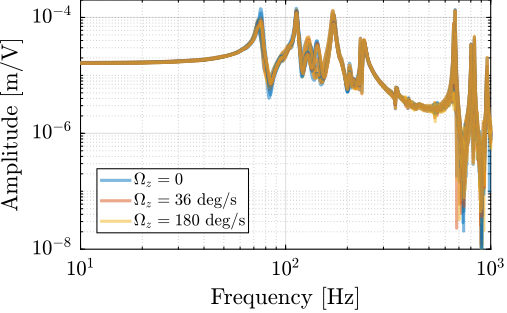

TODO Identification of Spurious modes

• These are made to identify the modes of the spheres
• Also discuss other observed modes

%% Load identification data
% mat_dir = "/home/thomas/mnt/data_id31/nass";
data = load(sprintf('%s/dynamics/2023-08-10_18-32_identify_spurious_modes.mat', mat_dir));

Conclusion

Thanks to the model, poor alignment between the nano-hexapod axes and the external metrology axes could be identified. After alignment, the identified dynamics is well matching with the multi-body model.

Also, the observed effects of the payload mass and of the spindle rotation on the dynamics are well matching the model predictions.

Decentralized Integral Force Feedback

<<sec:test_id31_iff>>

Introduction   ignore

Before implementing a position controller, an active damping controller was first implemented as shown in Figure ref:fig:test_id31_iff_block_diagram. It consisted of a decentralized Integral Force Feedback controller $\bm{K}_{\text{IFF}}$, with all the diagonal terms being equal eqref:eq:test_id31_Kiff.

\begin{equation}\label{eq:test_id31_iff_diagonal} \bm{K}_{\text{IFF}} = K_{\text{IFF}} ⋅ \bm{I}_6 = \begin{bmatrix} K_{\text{IFF}} & & 0
& \ddots &
0 & & K_{\text{IFF}}

\end{bmatrix}

\end{equation}

\begin{tikzpicture}
  % Blocs
  \node[block={2.0cm}{2.0cm}] (P) {Plant};
  \coordinate[] (input)   at ($(P.south west)!0.5!(P.north west)$);
  \coordinate[] (outputH) at ($(P.south east)!0.2!(P.north east)$);
  \coordinate[] (outputL) at ($(P.south east)!0.8!(P.north east)$);

  \node[block, above=0.6 of P] (Klac) {$\bm{K}_\text{IFF}$};
  \node[addb, left= of input] (addF) {};

  % Connections and labels
  \draw[->] (outputL) -- ++(0.6, 0) coordinate(eastlac) |- (Klac.east);
  \node[above right] at (outputL){$\bm{V}_s$};
  \draw[->] (Klac.west) -| (addF.north);
  \draw[->] (addF.east) -- (input) node[above left]{$\bm{u}$};

  \draw[->] (outputH) -- ++(1.6, 0) node[above left]{$\bm{\epsilon}_{\mathcal{L}}$};
  \draw[<-] (addF.west) -- ++(-1.0, 0) node[above right]{$\bm{u}^{\prime}$};

  \begin{scope}[on background layer]
    \node[fit={(Klac.north-|eastlac) (addF.west|-P.south)}, fill=black!20!white, draw, dashed, inner sep=10pt] (Pi) {};
    \node[anchor={north west}] at (Pi.north west){$\text{Damped Plant}$};
  \end{scope}
\end{tikzpicture}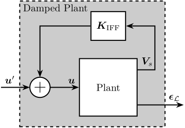

Block diagram of the implemented decentralized IFF controller. The controller $\bm{K}_{\text{IFF}}$ is a diagonal controller with the same elements on every diagonal term $K_{\text{IFF}}$.

IFF Plant

<<ssec:test_id31_iff_plant>>

As the multi-body model is going to be used to estimate the stability of the IFF controller and to optimize achievable damping, it is first checked is this model accurately represents the system dynamics.

In Figure ref:fig:test_id31_comp_simscape_iff_diag_masses, it was shown that the model well captures the dynamics from each actuator to its collocated force sensor, as that for all considered payloads. The model is also accurate for the dynamics from an actuator to the force sensors in the other struts (i.e. the off-diagonal dynamics) as shown in Figure ref:fig:test_id31_comp_simscape_Vs.

% Load identified FRF for IFF Plant and Multi-Body Model
load('test_id31_identified_open_loop_plants.mat', 'G_iff_m0_Wz0', 'G_iff_m1_Wz0', 'G_iff_m2_Wz0', 'G_iff_m3_Wz0', 'f');
load('test_id31_simscape_open_loop_plants.mat', 'Gm_m0_Wz0', 'Gm_m1_Wz0', 'Gm_m2_Wz0', 'Gm_m3_Wz0');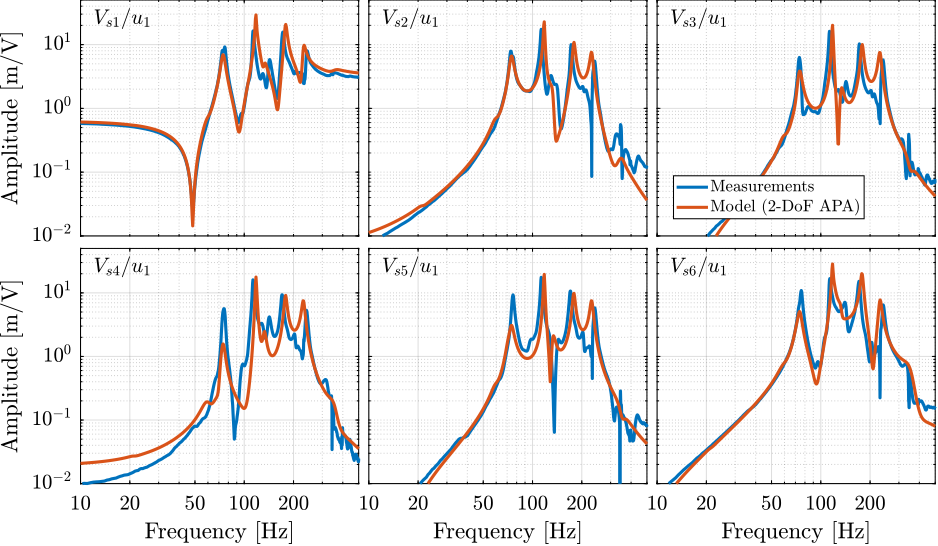

Comparison of the measured (in blue) and modeled (in red) frequency transfer functions from the first control signal $u_1$ to the six force sensor voltages $V_{s1}$ to $V_{s6}$

IFF Controller

<<ssec:test_id31_iff_controller>>

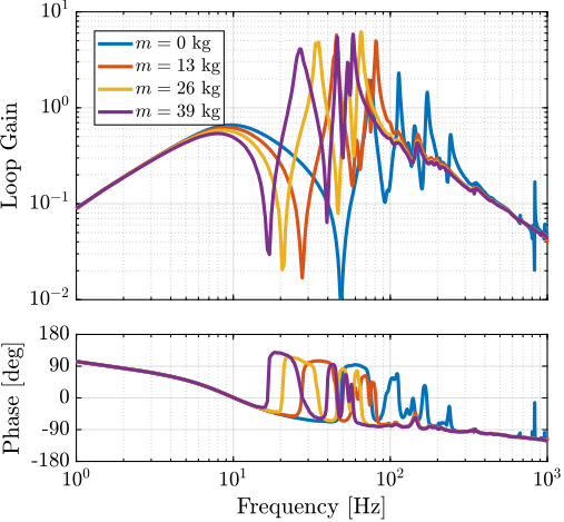
A decentralized IFF controller is there designed such that it adds damping to the suspension modes of the nano-hexapod for all considered payloads. The frequency of the suspension modes are ranging from $\approx 30\,\text{Hz}$ to $\approx 250\,\text{Hz}$ (Figure ref:fig:test_id31_comp_simscape_iff_diag_masses), and therefore the IFF controller should provide integral action in this frequency range. A second order high pass filter (cut-off frequency of $10\,\text{Hz}$) is added to limit the low frequency gain.

The bode plot of the decentralized IFF controller is shown in Figure ref:fig:test_id31_Kiff_bode_plot and the "decentralized loop-gains" for all considered payload masses are shown in Figure ref:fig:test_id31_Kiff_loop_gain. It can be seen that the loop-gain is larger than $1$ around suspension modes indicating that some damping should be added to the suspension modes.

\begin{equation}\label{eq:test_id31_Kiff} K_{\text{IFF}} = g_0 ⋅ _brace{\frac{1}{s}}_{\text{int}} ⋅ _brace{\frac{s^2/ω_z^2}{s^2/ω_z^2 + 2ξ_z s /ω_z + 1}}_{\text{2nd order LPF}},\quad ≤ft(g_0 = -100,\ ω_z = 2π10\,\text{rad/s},\ ξ_z = 0.7\right)

\end{equation}

%% IFF Controller Design
% Second order high pass filter
wz = 2*pi*10;
xiz = 0.7;
Ghpf = (s^2/wz^2)/(s^2/wz^2 + 2*xiz*s/wz + 1);

% IFF Controller
Kiff = -1e2 * ...              % Gain
       1/(0.01*2*pi + s) * ... % LPF: provides integral action
       Ghpf * ...              % 2nd order HPF (limit low frequency gain)
       eye(6);                 % Diagonal 6x6 controller (i.e. decentralized)

Kiff.InputName = {'Vs1', 'Vs2', 'Vs3', 'Vs4', 'Vs5', 'Vs6'};
Kiff.OutputName = {'u1', 'u2', 'u3', 'u4', 'u5', 'u6'};

% The designed IFF controller is saved
save('./mat/test_id31_K_iff.mat', 'Kiff');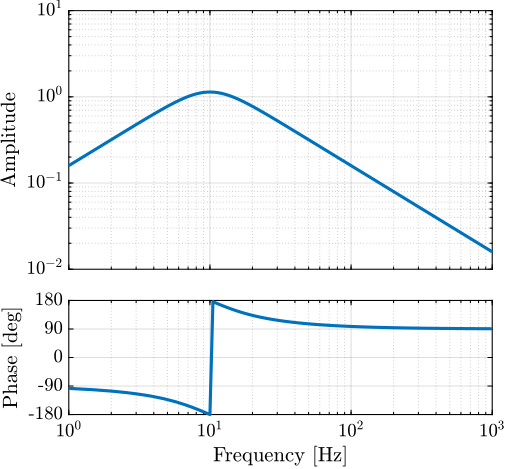

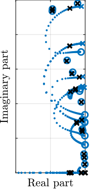
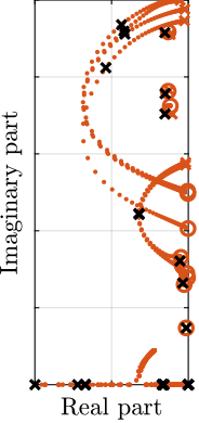
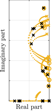
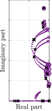
To estimate the added damping, a root-locus plot is computed using the multi-body model (Figure ref:fig:test_id31_iff_root_locus_m0). It can be seen that for all considered payloads, the poles are bounded to the "left-half plane" indicating that the decentralized IFF is robust. The closed-loop poles for the chosen value of the gain are displayed by black crosses. It can be seen that while damping can be added for all payloads (as compared to the open-loop case), the optimal value of the gain could be tuned separately for each payload. For instance, for low payload masses, a higher value of the IFF controller gain could lead to better damping. However, in this study, it was chosen to implement a fix (i.e. non-adaptive) decentralized IFF controller.

Estimated Damped Plant

<<ssec:test_id31_iff_perf>>

As the model is accurately modelling the system dynamics, it can be used to estimate the damped plant, i.e. the transfer functions from $\bm{u}^\prime$ to $\bm{\mathcal{L}}$. The obtained damped plants are compared with the open-loop plants in Figure ref:fig:test_id31_comp_ol_iff_plant_model. The peak amplitudes corresponding to the suspension modes are approximately reduced by a factor $10$ for all considered payloads, and with the same decentralized IFF controller.

%% Estimate damped plant from Multi-Body model
Gm_hac_m0_Wz0 = feedback(Gm_m0_Wz0, Kiff, 'name', +1);
Gm_hac_m1_Wz0 = feedback(Gm_m1_Wz0, Kiff, 'name', +1);
Gm_hac_m2_Wz0 = feedback(Gm_m2_Wz0, Kiff, 'name', +1);
Gm_hac_m3_Wz0 = feedback(Gm_m3_Wz0, Kiff, 'name', +1);

% Check Stability
isstable(Gm_hac_m0_Wz0)
isstable(Gm_hac_m1_Wz0)
isstable(Gm_hac_m2_Wz0)
isstable(Gm_hac_m3_Wz0)

% The estimated damped plants from the multi-body model are saved
save('./mat/test_id31_simscape_damped_plants.mat', 'Gm_hac_m0_Wz0', 'Gm_hac_m1_Wz0', 'Gm_hac_m2_Wz0', 'Gm_hac_m3_Wz0');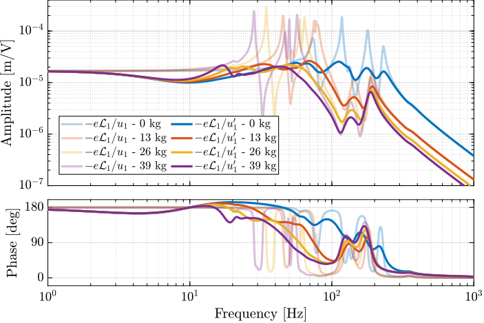

Comparison of the open-loop plants and the estimated damped plant with Decentralized IFF.

Conclusion

High Authority Control in the frame of the struts

<<sec:test_id31_iff_hac>>

Introduction   ignore

The position of the sample is actively stabilized by implementing a High-Authority-Controller as shown in Figure ref:fig:test_id31_iff_hac_schematic.

\begin{equation}\label{eq:eq:test_id31_hac_diagonal} \bm{K}_{\text{HAC}} = K_{\text{HAC}} ⋅ \bm{I}_6 = \begin{bmatrix} K_{\text{HAC}} & & 0
& \ddots &
0 & & K_{\text{HAC}}

\end{bmatrix}

\end{equation}

\begin{tikzpicture}
  % Blocs
  \node[block={2.0cm}{2.0cm}] (P) {Plant};
  \coordinate[] (input)   at ($(P.south west)!0.5!(P.north west)$);
  \coordinate[] (outputH) at ($(P.south east)!0.2!(P.north east)$);
  \coordinate[] (outputL) at ($(P.south east)!0.8!(P.north east)$);

  \node[block, above=0.6 of P] (Klac) {$\bm{K}_\text{IFF}$};
  \node[addb, left= of input] (addF) {};

  \node[block, left= of addF] (Khac) {$\bm{K}_\text{HAC}$};

  % Connections and labels
  \draw[->] (outputL) -- ++(0.6, 0) coordinate(eastlac) |- (Klac.east);
  \node[above right] at (outputL){$\bm{V}_s$};
  \draw[->] (Klac.west) -| (addF.north);
  \draw[->] (addF.east) -- (input) node[above left]{$\bm{u}$};

  \draw[->] (outputH) -- ++(1.6, 0) node[above left]{$\bm{\epsilon\mathcal{L}}$};
  \draw[->] (Khac.east) node[above right]{$\bm{u}^{\prime}$} -- (addF.west);

  \draw[->] ($(outputH) + (1.2, 0)$)node[branch]{} |- ($(Khac.west)+(-0.6, -1.6)$) |- (Khac.west);

  \begin{scope}[on background layer]
    \node[fit={(Klac.north-|eastlac) (addF.west|-P.south)}, fill=black!20!white, draw, dashed, inner sep=10pt] (Pi) {};
    \node[anchor={north west}] at (Pi.north west){$\text{Damped Plant}$};
  \end{scope}
\end{tikzpicture}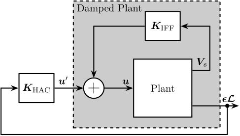

Block diagram of the implemented HAC-IFF controllers. The controller $\bm{K}_{\text{HAC}}$ is a diagonal controller with the same elements on every diagonal term $K_{\text{HAC}}$.

Damped Plant

<<ssec:test_id31_iff_hac_plant>>

The damped plants (i.e. the transfer function from $\bm{u}^\prime$ to $\bm{\epsilon\mathcal{L}}$) were identified for all payload conditions. To verify if the model accurately represents the damped plants, both direct terms and coupling terms corresponding to the first actuator are compared in Figure ref:fig:test_id31_comp_simscape_hac.

%% Identification of the damped Plant (transfer function from u' to dL)

% Load identification data
data_m0 = load('2023-08-17_17-53_damp_plant_m0_Wz0.mat');
data_m1 = load('2023-08-10_16-01_damp_plant_m1_Wz0.mat');
data_m2 = load('2023-08-10_17-28_damp_plant_m2_Wz0.mat');
data_m3 = load('2023-08-10_18-16_damp_plant_m3_Wz0.mat');

% Hannning Windows
Ts = 1e-4; % Sampling Time [s]
Nfft = floor(2.0/Ts);
win = hanning(Nfft);
Noverlap = floor(Nfft/2);

% And we get the frequency vector
[~, f] = tfestimate(data_m0.uL1.id_plant, data_m0.uL1.e_L1, win, Noverlap, Nfft, 1/Ts);

% Identification without any payload
G_hac_m0_Wz0 = zeros(length(f), 6, 6);
for i_strut = 1:6
    eL = [data_m0.(sprintf("uL%i", i_strut)).e_L1 ; data_m0.(sprintf("uL%i", i_strut)).e_L2 ; data_m0.(sprintf("uL%i", i_strut)).e_L3 ; data_m0.(sprintf("uL%i", i_strut)).e_L4 ; data_m0.(sprintf("uL%i", i_strut)).e_L5 ; data_m0.(sprintf("uL%i", i_strut)).e_L6]';

    G_hac_m0_Wz0(:,:,i_strut) = tfestimate(data_m0.(sprintf("uL%i", i_strut)).id_plant, -detrend(eL, 0), win, Noverlap, Nfft, 1/Ts);
end

% Identification with 1 "payload layer"
G_hac_m1_Wz0 = zeros(length(f), 6, 6);
for i_strut = 1:6
    eL = [data_m1.(sprintf("uL%i", i_strut)).e_L1 ; data_m1.(sprintf("uL%i", i_strut)).e_L2 ; data_m1.(sprintf("uL%i", i_strut)).e_L3 ; data_m1.(sprintf("uL%i", i_strut)).e_L4 ; data_m1.(sprintf("uL%i", i_strut)).e_L5 ; data_m1.(sprintf("uL%i", i_strut)).e_L6]';

    G_hac_m1_Wz0(:,:,i_strut) = tfestimate(data_m1.(sprintf("uL%i", i_strut)).id_plant, -detrend(eL, 0), win, Noverlap, Nfft, 1/Ts);
end

% Identification with 2 "payload layers"
G_hac_m2_Wz0 = zeros(length(f), 6, 6);
for i_strut = 1:6
    eL = [data_m2.(sprintf("uL%i", i_strut)).e_L1 ; data_m2.(sprintf("uL%i", i_strut)).e_L2 ; data_m2.(sprintf("uL%i", i_strut)).e_L3 ; data_m2.(sprintf("uL%i", i_strut)).e_L4 ; data_m2.(sprintf("uL%i", i_strut)).e_L5 ; data_m2.(sprintf("uL%i", i_strut)).e_L6]';

    G_hac_m2_Wz0(:,:,i_strut) = tfestimate(data_m2.(sprintf("uL%i", i_strut)).id_plant, -detrend(eL, 0), win, Noverlap, Nfft, 1/Ts);
end

% Identification with 3 "payload layers"
G_hac_m3_Wz0 = zeros(length(f), 6, 6);
for i_strut = 1:6
    eL = [data_m3.(sprintf("uL%i", i_strut)).e_L1 ; data_m3.(sprintf("uL%i", i_strut)).e_L2 ; data_m3.(sprintf("uL%i", i_strut)).e_L3 ; data_m3.(sprintf("uL%i", i_strut)).e_L4 ; data_m3.(sprintf("uL%i", i_strut)).e_L5 ; data_m3.(sprintf("uL%i", i_strut)).e_L6]';

    G_hac_m3_Wz0(:,:,i_strut) = tfestimate(data_m3.(sprintf("uL%i", i_strut)).id_plant, -detrend(eL, 0), win, Noverlap, Nfft, 1/Ts);
end

% The identified dynamics are then saved for further use.
save('./mat/test_id31_identified_damped_plants.mat', 'G_hac_m0_Wz0', 'G_hac_m1_Wz0', 'G_hac_m2_Wz0', 'G_hac_m3_Wz0', 'f');

% Load the estimated damped plant from the multi-body model
load('test_id31_simscape_damped_plants.mat', 'Gm_hac_m0_Wz0', 'Gm_hac_m1_Wz0', 'Gm_hac_m2_Wz0', 'Gm_hac_m3_Wz0');
% Load the undamped plant for comparison
load('test_id31_identified_open_loop_plants.mat', 'G_int_m0_Wz0', 'G_int_m1_Wz0', 'G_int_m2_Wz0', 'G_int_m3_Wz0', 'f');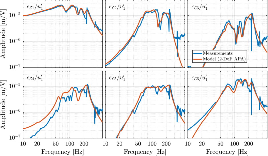

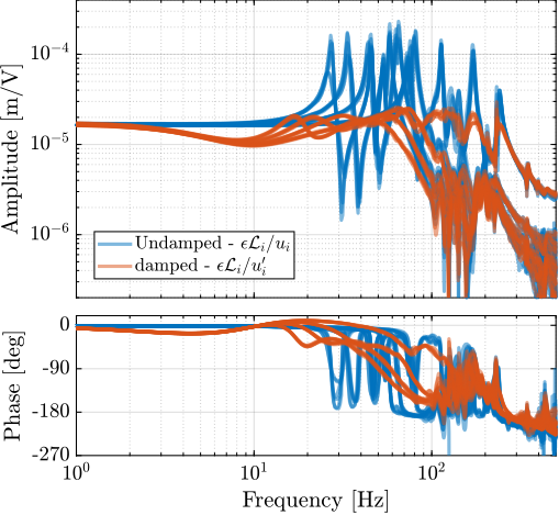
Comparison of the measured (in blue) and modeled (in red) frequency transfer functions from the first control signal ($u_1^\prime$) of the damped plant to the estimated errors ($\epsilon_{\mathcal{L}_i}$) in the frame of the six struts by the external metrology

The six direct terms for all four payload conditions are compared with the model in Figure ref:fig:test_id31_hac_plant_effect_mass. It is shown that the model accurately represents the dynamics for all payloads.

In Section ref:sec:test_id31_iff_hac, a High Authority Controller is tuned to be robust to the change of dynamics due to different payloads used. Without decentralized IFF being applied, the controller would have had to be robust to all the undamped dynamics shown in Figure ref:fig:test_id31_comp_all_undamped_damped_plants, which is a very complex control problem. With the applied decentralized IFF, the HAC instead had to be be robust to all the damped dynamics shown in Figure ref:fig:test_id31_comp_all_undamped_damped_plants, which is easier from a control perspective. This is one of the key benefit of using the HAC-LAC strategy.

Robust Controller Design

<<ssec:test_id31_iff_hac_controller>>

A first diagonal controller was designed to be robust to change of payloads, which means that every damped plants shown in Figure ref:fig:test_id31_comp_all_undamped_damped_plants should be considered during the controller design. For a first design, a crossover frequency of $5\,\text{Hz}$ for chosen. One integrator is added to increase the low frequency gain, a lead is added around $5\,\text{Hz}$ to increase the stability margins and a first order low pass filter with a cut-off frequency of $30\,\text{Hz}$ is added to improve the robustness to dynamical uncertainty at high frequency. The obtained "decentralized" loop-gains are shown in Figure ref:fig:test_id31_hac_loop_gain.

\begin{equation}\label{eq:test_id31_robust_hac} K_{\text{HAC}} = g_0 ⋅ _brace{\frac{ω_c}{s}}_{\text{int}} ⋅ _brace{\frac{1}{\sqrt{α}}\frac{1 + \frac{s}{ω_c/\sqrt{α}}}{1 + \frac{s}{ω_c\sqrt{α}}}}_{\text{lead}} ⋅ _brace{\frac{1}{1 + \frac{s}{ω_0}}}_{\text{LPF}}, \quad ≤ft( ω_c = 2π5\,\text{rad/s},\ α = 2,\ ω_0 = 2π30\,\text{rad/s} \right)

\end{equation}

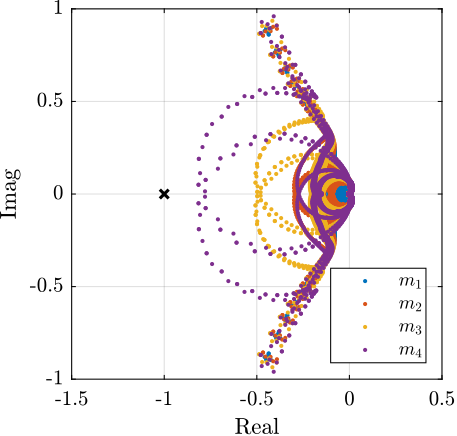
The closed-loop stability is verified by computing the characteristic Loci (Figure ref:fig:test_id31_hac_characteristic_loci).

%% HAC Design
% Wanted crossover
wc = 2*pi*5; % [rad/s]

% Integrator
H_int = wc/s;

% Lead to increase phase margin
a  = 2;  % Amount of phase lead / width of the phase lead / high frequency gain
H_lead = 1/sqrt(a)*(1 + s/(wc/sqrt(a)))/(1 + s/(wc*sqrt(a)));

% Low Pass filter to increase robustness
H_lpf = 1/(1 + s/2/pi/30);

% Gain to have unitary crossover at 5Hz
[~, i_f] = min(abs(f - wc/2/pi));
H_gain = 1./abs(G_hac_m0_Wz0(i_f, 1, 1));

% Decentralized HAC
Khac = H_gain  * ... % Gain
       H_int   * ... % Integrator
       H_lpf   * ... % Low Pass filter
       eye(6);       % 6x6 Diagonal

% The designed HAC controller is saved
save('./mat/test_id31_K_hac_robust.mat', 'Khac');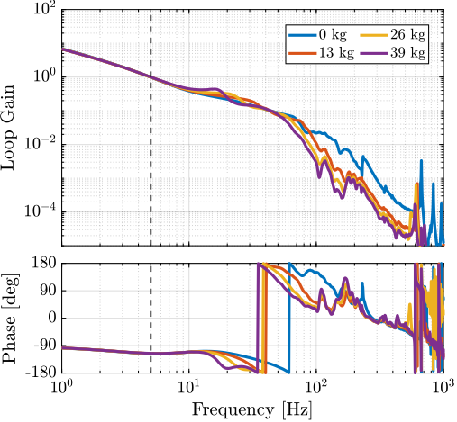

Estimation of performances

<<ssec:test_id31_iff_hac_perf>>

To estimate the performances that can be expected with this HAC-LAC architecture and the designed controllers, two simulations of tomography experiments were performed⁴. The rotational velocity was set to 30rpm, and no payload was added on top of the nano-hexapod. An open-loop simulation and a closed-loop simulation were performed and compared in Figure ref:fig:test_id31_tomo_m0_30rpm_robust_hac_iff_sim.

%% Tomography experiment
% Sample is not centered with the rotation axis
% This is done by offsetfing the micro-hexapod by 0.9um
P_micro_hexapod = [2.5e-6; 0; -0.3e-6]; % [m]

set_param(mdl, 'StopTime', '3'); % 6 turns at 30rpm

initializeGround();
initializeGranite();
initializeTy();
initializeRy();
initializeRz();
initializeMicroHexapod('AP', P_micro_hexapod);
initializeNanoHexapod('flex_bot_type', '2dof', ...
                      'flex_top_type', '3dof', ...
                      'motion_sensor_type', 'plates', ...
                      'actuator_type', '2dof');
initializeSample('type', '0');

initializeSimscapeConfiguration('gravity', false);
initializeLoggingConfiguration('log', 'all', 'Ts', 1e-4);
initializeController('type', 'open-loop');

initializeDisturbances(...
    'Dw_x',  true, ... % Ground Motion - X direction
    'Dw_y',  true, ... % Ground Motion - Y direction
    'Dw_z',  true, ... % Ground Motion - Z direction
    'Fdy_x', false, ... % Translation Stage - X direction
    'Fdy_z', false, ... % Translation Stage - Z direction
    'Frz_x', true, ... % Spindle - X direction
    'Frz_y', true, ... % Spindle - Y direction
    'Frz_z', true);    % Spindle - Z direction

initializeReferences(...
    'Rz_type', 'rotating', ...
    'Rz_period', 360/180, ... % 180deg/s, 30rpm
    'Dh_pos', [P_micro_hexapod; 0; 0; 0]);

% Open-Loop Simulation
sim(mdl);
exp_tomo_ol_m0_Wz180 = simout;

% Closed-Loop Simulation
load('test_id31_K_iff.mat', 'Kiff');
load('test_id31_K_hac_robust.mat', 'Khac');
initializeController('type', 'hac-iff');
initializeSample('type', '0');
sim(mdl);
exp_tomo_cl_m0_Wz180 = simout;

% Save the simulation results
save('./mat/test_id31_exp_tomo_ol_cl_30rpm_sim.mat', 'exp_tomo_ol_m0_Wz180', 'exp_tomo_cl_m0_Wz180');

Then the same tomography experiment (i.e. constant spindle rotation at 30rpm, and no payload) was performed experimentally. The measured position of the "point of interest" during the experiment are shown in Figure ref:fig:test_id31_tomo_m0_30rpm_robust_hac_iff_exp.

%% Experimental Results for Tomography at 30RPM, no payload
% Load measured noise
data_tomo_m0_Wz180 = load('2023-08-17_15-26_tomography_30rpm_m0_robust.mat');

[~, i_cl] = find(data_tomo_m0_Wz180.hac_status == 1);

Even though the simulation (Figure ref:fig:test_id31_tomo_m0_30rpm_robust_hac_iff_sim) and the experimental results (Figure ref:fig:test_id31_tomo_m0_30rpm_robust_hac_iff_exp) are looking similar, the most important metric to compare is the RMS values of the positioning errors in closed-loop. These are computed for both the simulation and the experimental results and are compared in Table ref:tab:test_id31_tomo_m0_30rpm_robust_hac_iff_rms. The lateral and vertical errors are similar, however the tilt ($R_y$) errors are underestimated by the model, which is reasonable as disturbances in $R_y$ were not modeled.

Results obtained with this conservative HAC are already close to the specifications.

%% Compute RMS of errors

% Simulation - OL
rms_Dy_m0_Wz180_ol_sim = rms(detrend(exp_tomo_ol_m0_Wz180.y.y.Data, 0));
rms_Dz_m0_Wz180_ol_sim = rms(detrend(exp_tomo_ol_m0_Wz180.y.z.Data, 0));
rms_Ry_m0_Wz180_ol_sim = rms(detrend(squeeze(atan2(exp_tomo_ol_m0_Wz180.y.R.Data(1,3,:), sqrt(exp_tomo_ol_m0_Wz180.y.R.Data(1,1,:).^2+exp_tomo_ol_m0_Wz180.y.R.Data(1,2,:).^2))), 0));
i_stab = 1000; % Remove the transient that is irrelevant here
% Simulation - CL
rms_Dy_m0_Wz180_cl_sim = rms(detrend(exp_tomo_cl_m0_Wz180.y.y.Data(i_stab:end), 0));
rms_Dz_m0_Wz180_cl_sim = rms(detrend(exp_tomo_cl_m0_Wz180.y.z.Data(i_stab:end), 0));
rms_Ry_m0_Wz180_cl_sim = rms(detrend(squeeze(atan2(exp_tomo_cl_m0_Wz180.y.R.Data(1,3,i_stab:end), sqrt(exp_tomo_cl_m0_Wz180.y.R.Data(1,1,i_stab:end).^2+exp_tomo_cl_m0_Wz180.y.R.Data(1,2,i_stab:end).^2))), 0));

% Experimental - OL
[~, i_cl] = find(data_tomo_m0_Wz180.hac_status == 1);
rms_Dy_m0_Wz180_ol_exp = rms(detrend(data_tomo_m0_Wz180.Dy_int(1:i_cl), 0));
rms_Dz_m0_Wz180_ol_exp = rms(detrend(data_tomo_m0_Wz180.Dz_int(1:i_cl), 0));
rms_Ry_m0_Wz180_ol_exp = rms(detrend(data_tomo_m0_Wz180.Ry_int(1:i_cl), 0));
% Experimental - CL
rms_Dy_m0_Wz180_cl_exp = rms(detrend(data_tomo_m0_Wz180.Dy_int(i_cl+10000:end), 0));
rms_Dz_m0_Wz180_cl_exp = rms(detrend(data_tomo_m0_Wz180.Dz_int(i_cl+10000:end), 0));
rms_Ry_m0_Wz180_cl_exp = rms(detrend(data_tomo_m0_Wz180.Ry_int(i_cl+10000:end), 0));

	$D_y$	$D_z$	$R_y$
Experiment (OL)	$1.8\,\mu\text{mRMS}$	$24\,\text{nmRMS}$	$10\,\mu\text{radRMS}$
Simulation (CL)	$30\,\text{nmRMS}$	$8\,\text{nmRMS}$	$73\,\text{nradRMS}$
Experiment (CL)	$39\,\text{nmRMS}$	$11\,\text{nmRMS}$	$130\,\text{nradRMS}$
Specifications (CL)	$30\,\text{nmRMS}$	$15\,\text{nmRMS}$	$250\,\text{nradRMS}$

Robustness to change of payload

<<ssec:test_id31_iff_hac_robustness>>

To verify the robustness to the change of payload mass, four simulations of tomography experiments were performed with payloads as shown Figure ref:fig:test_id31_picture_masses (i.e. $0\,kg$, $13\,kg$, $26\,kg$ and $39\,kg$). This time, the rotational velocity was set at 1rpm (i.e. 6deg/s), as it is the typical rotational velocity for heavy samples. The closed-loop systems were stable for all payload conditions, indicating good control robustness.

%% Simulation of tomography experiments at 1RPM with all payloads

% Configuration
set_param(mdl, 'StopTime', '2'); % 30 degrees at 1rpm
initializeLoggingConfiguration('log', 'all', 'Ts', 1e-3);
initializeController('type', 'hac-iff');
initializeReferences(...
    'Rz_type', 'rotating', ...
    'Rz_period', 360/6, ... % 6deg/s, 1 rpm
    'Dh_pos', [P_micro_hexapod; 0; 0; 0]);

% Perform the simulations
initializeSample('type', '0');
sim(mdl);
exp_tomo_cl_m0_1rpm = simout;
initializeSample('type', '1');
sim(mdl);
exp_tomo_cl_m1_1rpm = simout;
initializeSample('type', '2');
sim(mdl);
exp_tomo_cl_m2_1rpm = simout;
initializeSample('type', '3');
sim(mdl);
exp_tomo_cl_m3_1rpm = simout;

% Save the simulation results
save('./mat/test_id31_exp_tomo_cl_1rpm_sim.mat', 'exp_tomo_cl_m0_1rpm', 'exp_tomo_cl_m1_1rpm', 'exp_tomo_cl_m2_1rpm', 'exp_tomo_cl_m3_1rpm');

figure;
hold on;
plot(exp_tomo_cl_m3_1rpm.y.x.Data, exp_tomo_cl_m3_1rpm.y.y.Data)
plot(exp_tomo_cl_m2_1rpm.y.x.Data, exp_tomo_cl_m2_1rpm.y.y.Data)
plot(exp_tomo_cl_m1_1rpm.y.x.Data, exp_tomo_cl_m1_1rpm.y.y.Data)
plot(exp_tomo_cl_m0_1rpm.y.x.Data, exp_tomo_cl_m0_1rpm.y.y.Data)

% Estimate the RMS value of the errors
i_stab = 1000; % Remove the transient that is irrelevant here
rms_Dy_m0_1rpm = rms(detrend(exp_tomo_cl_m0_1rpm.y.y.Data(i_stab:end), 0));
rms_Dz_m0_1rpm = rms(detrend(exp_tomo_cl_m0_1rpm.y.z.Data(i_stab:end), 0));
rms_Ry_m0_1rpm = rms(detrend(squeeze(atan2(exp_tomo_cl_m0_1rpm.y.R.Data(1,3,:), sqrt(exp_tomo_cl_m0_1rpm.y.R.Data(1,1,:).^2+exp_tomo_cl_m0_1rpm.y.R.Data(1,2,:).^2))), 0));
rms_Dy_m1_1rpm = rms(detrend(exp_tomo_cl_m1_1rpm.y.y.Data(i_stab:end), 0));
rms_Dz_m1_1rpm = rms(detrend(exp_tomo_cl_m1_1rpm.y.z.Data(i_stab:end), 0));
rms_Ry_m1_1rpm = rms(detrend(squeeze(atan2(exp_tomo_cl_m1_1rpm.y.R.Data(1,3,:), sqrt(exp_tomo_cl_m1_1rpm.y.R.Data(1,1,:).^2+exp_tomo_cl_m1_1rpm.y.R.Data(1,2,:).^2))), 0));
rms_Dy_m2_1rpm = rms(detrend(exp_tomo_cl_m2_1rpm.y.y.Data(i_stab:end), 0));
rms_Dz_m2_1rpm = rms(detrend(exp_tomo_cl_m2_1rpm.y.z.Data(i_stab:end), 0));
rms_Ry_m2_1rpm = rms(detrend(squeeze(atan2(exp_tomo_cl_m2_1rpm.y.R.Data(1,3,:), sqrt(exp_tomo_cl_m2_1rpm.y.R.Data(1,1,:).^2+exp_tomo_cl_m2_1rpm.y.R.Data(1,2,:).^2))), 0));
rms_Dy_m3_1rpm = rms(detrend(exp_tomo_cl_m3_1rpm.y.y.Data(i_stab:end), 0));
rms_Dz_m3_1rpm = rms(detrend(exp_tomo_cl_m3_1rpm.y.z.Data(i_stab:end), 0));
rms_Ry_m3_1rpm = rms(detrend(squeeze(atan2(exp_tomo_cl_m3_1rpm.y.R.Data(1,3,:), sqrt(exp_tomo_cl_m3_1rpm.y.R.Data(1,1,:).^2+exp_tomo_cl_m3_1rpm.y.R.Data(1,2,:).^2))), 0));

The tomography experiments that were simulated were then experimentally conducted. For each payload, a spindle rotating was first performed in open-loop, and then the loop was closed during another full spindle rotation. An example with the $26\,\text{kg}$ payload is shown in Figure ref:fig:test_id31_tomo_m2_1rpm_robust_hac_iff_fit. The eccentricity between the "point of interest" and the spindle rotation axis is quite large as the added payload mass statically deforms the micro-station stages. To estimate the open-loop errors, it is supposed that the "point of interest" can be perfectly aligned with the spindle rotation axis. Therefore, the eccentricity is first estimated by performing a circular fit (dashed black circle in Figure ref:fig:test_id31_tomo_m2_1rpm_robust_hac_iff_fit), and then subtracted from the data in Figure ref:fig:test_id31_tomo_m2_1rpm_robust_hac_iff_fit_removed. This underestimate the real condition open-loop errors as it is difficult to obtain a perfect alignment in practice.

%% Load Tomography scans with robust controller
data_tomo_m0_Wz6 = load("2023-08-11_11-37_tomography_1rpm_m0.mat");
data_tomo_m0_Wz6.time = Ts*[0:length(data_tomo_m0_Wz6.Rz)-1];

data_tomo_m1_Wz6 = load("2023-08-11_11-15_tomography_1rpm_m1.mat");
data_tomo_m1_Wz6.time = Ts*[0:length(data_tomo_m1_Wz6.Rz)-1];

data_tomo_m2_Wz6 = load("2023-08-11_10-59_tomography_1rpm_m2.mat");
data_tomo_m2_Wz6.time = Ts*[0:length(data_tomo_m2_Wz6.Rz)-1];

data_tomo_m3_Wz6 = load("2023-08-11_10-24_tomography_1rpm_m3.mat");
data_tomo_m3_Wz6.time = Ts*[0:length(data_tomo_m3_Wz6.Rz)-1];

The RMS values of the open-loop and closed-loop errors for all masses are summarized in Table ref:tab:test_id31_tomo_1rpm_robust_ol_cl_errors. The obtained closed-loop errors are fulfilling the requirements, except for the $39\,\text{kg}$ payload in the lateral ($D_y$) direction.

%% Estimate RMS of the errors while in closed-loop and open-loop
% No mass
[~, i_m0] = find(data_tomo_m0_Wz6.hac_status == 1);
data_tomo_m0_Wz6.Dy_rms_cl = rms(detrend(data_tomo_m0_Wz6.Dy_int(i_m0+50000:end), 0));
data_tomo_m0_Wz6.Dz_rms_cl = rms(detrend(data_tomo_m0_Wz6.Dz_int(i_m0+50000:end), 0));
data_tomo_m0_Wz6.Ry_rms_cl = rms(detrend(data_tomo_m0_Wz6.Ry_int(i_m0+50000:end), 0));

% Remove eccentricity for OL errors
[x0, y0, R] = circlefit(data_tomo_m0_Wz6.Dx_int(1:i_m0), data_tomo_m0_Wz6.Dy_int(1:i_m0));
fun = @(theta)rms((data_tomo_m0_Wz6.Dx_int(1:i_m0) - (x0 + R*cos(data_tomo_m0_Wz6.Rz(1:i_m0)+theta(1)))).^2 + ...
                  (data_tomo_m0_Wz6.Dy_int(1:i_m0) - (y0 + R*sin(data_tomo_m0_Wz6.Rz(1:i_m0)+theta(1)))).^2);
delta_theta = fminsearch(fun, 0);
data_tomo_m0_Wz6.Dy_rms_ol = rms(data_tomo_m0_Wz6.Dy_int(1:i_m0) - (y0 + R*sin(data_tomo_m0_Wz6.Rz(1:i_m0)+delta_theta)));
data_tomo_m0_Wz6.Dz_rms_ol = rms(detrend(data_tomo_m0_Wz6.Dz_int(1:i_m0), 0));
[x0, y0, R] = circlefit(data_tomo_m0_Wz6.Rx_int(1:i_m0), data_tomo_m0_Wz6.Ry_int(1:i_m0));
fun = @(theta)rms((data_tomo_m0_Wz6.Rx_int(1:i_m0) - (x0 + R*cos(data_tomo_m0_Wz6.Rz(1:i_m0)+theta(1)))).^2 + ...
                  (data_tomo_m0_Wz6.Ry_int(1:i_m0) - (y0 + R*sin(data_tomo_m0_Wz6.Rz(1:i_m0)+theta(1)))).^2);
delta_theta = fminsearch(fun, 0);
data_tomo_m0_Wz6.Ry_rms_ol = rms(data_tomo_m0_Wz6.Ry_int(1:i_m0) - (y0 + R*sin(data_tomo_m0_Wz6.Rz(1:i_m0)+delta_theta)));

% 1 "layer mass"
[~, i_m1] = find(data_tomo_m1_Wz6.hac_status == 1);
data_tomo_m1_Wz6.Dy_rms_cl = rms(detrend(data_tomo_m1_Wz6.Dy_int(i_m1+50000:end), 0));
data_tomo_m1_Wz6.Dz_rms_cl = rms(detrend(data_tomo_m1_Wz6.Dz_int(i_m1+50000:end), 0));
data_tomo_m1_Wz6.Ry_rms_cl = rms(detrend(data_tomo_m1_Wz6.Ry_int(i_m1+50000:end), 0));

% Remove eccentricity for OL errors
[x0, y0, R] = circlefit(data_tomo_m1_Wz6.Dx_int(1:i_m1), data_tomo_m1_Wz6.Dy_int(1:i_m1));
fun = @(theta)rms((data_tomo_m1_Wz6.Dx_int(1:i_m1) - (x0 + R*cos(data_tomo_m1_Wz6.Rz(1:i_m1)+theta(1)))).^2 + ...
                  (data_tomo_m1_Wz6.Dy_int(1:i_m1) - (y0 + R*sin(data_tomo_m1_Wz6.Rz(1:i_m1)+theta(1)))).^2);
delta_theta = fminsearch(fun, 0);
data_tomo_m1_Wz6.Dy_rms_ol = rms(data_tomo_m1_Wz6.Dy_int(1:i_m1) - (y0 + R*sin(data_tomo_m1_Wz6.Rz(1:i_m1)+delta_theta)));
data_tomo_m1_Wz6.Dz_rms_ol = rms(detrend(data_tomo_m1_Wz6.Dz_int(1:i_m1), 0));
[x0, y0, R] = circlefit(data_tomo_m1_Wz6.Rx_int(1:i_m1), data_tomo_m1_Wz6.Ry_int(1:i_m1));
fun = @(theta)rms((data_tomo_m1_Wz6.Rx_int(1:i_m1) - (x0 + R*cos(data_tomo_m1_Wz6.Rz(1:i_m1)+theta(1)))).^2 + ...
                  (data_tomo_m1_Wz6.Ry_int(1:i_m1) - (y0 + R*sin(data_tomo_m1_Wz6.Rz(1:i_m1)+theta(1)))).^2);
delta_theta = fminsearch(fun, 0);
data_tomo_m1_Wz6.Ry_rms_ol = rms(data_tomo_m1_Wz6.Ry_int(1:i_m1) - (y0 + R*sin(data_tomo_m1_Wz6.Rz(1:i_m1)+delta_theta)));

% 2 "layer masses"
[~, i_m2] = find(data_tomo_m2_Wz6.hac_status == 1);
data_tomo_m2_Wz6.Dy_rms_cl = rms(detrend(data_tomo_m2_Wz6.Dy_int(i_m2+50000:end), 0));
data_tomo_m2_Wz6.Dz_rms_cl = rms(detrend(data_tomo_m2_Wz6.Dz_int(i_m2+50000:end), 0));
data_tomo_m2_Wz6.Ry_rms_cl = rms(detrend(data_tomo_m2_Wz6.Ry_int(i_m2+50000:end), 0));

% Remove eccentricity for OL errors
[x0, y0, R] = circlefit(data_tomo_m2_Wz6.Dx_int(1:i_m2), data_tomo_m2_Wz6.Dy_int(1:i_m2));
fun = @(theta)rms((data_tomo_m2_Wz6.Dx_int(1:i_m2) - (x0 + R*cos(data_tomo_m2_Wz6.Rz(1:i_m2)+theta(1)))).^2 + ...
                  (data_tomo_m2_Wz6.Dy_int(1:i_m2) - (y0 + R*sin(data_tomo_m2_Wz6.Rz(1:i_m2)+theta(1)))).^2);
delta_theta = fminsearch(fun, 0);
data_tomo_m2_Wz6.Dy_rms_ol = rms(data_tomo_m2_Wz6.Dy_int(1:i_m2) - (y0 + R*sin(data_tomo_m2_Wz6.Rz(1:i_m2)+delta_theta)));
data_tomo_m2_Wz6.Dz_rms_ol = rms(detrend(data_tomo_m2_Wz6.Dz_int(1:i_m2), 0));
[x0, y0, R] = circlefit(data_tomo_m2_Wz6.Rx_int(1:i_m2), data_tomo_m2_Wz6.Ry_int(1:i_m2));
fun = @(theta)rms((data_tomo_m2_Wz6.Rx_int(1:i_m2) - (x0 + R*cos(data_tomo_m2_Wz6.Rz(1:i_m2)+theta(1)))).^2 + ...
                  (data_tomo_m2_Wz6.Ry_int(1:i_m2) - (y0 + R*sin(data_tomo_m2_Wz6.Rz(1:i_m2)+theta(1)))).^2);
delta_theta = fminsearch(fun, 0);
data_tomo_m2_Wz6.Ry_rms_ol = rms(data_tomo_m2_Wz6.Ry_int(1:i_m2) - (y0 + R*sin(data_tomo_m2_Wz6.Rz(1:i_m2)+delta_theta)));

% 3 "layer masses"
[~, i_m3] = find(data_tomo_m3_Wz6.hac_status == 1);
data_tomo_m3_Wz6.Dy_rms_cl = rms(detrend(data_tomo_m3_Wz6.Dy_int(i_m3+50000:end), 0));
data_tomo_m3_Wz6.Dz_rms_cl = rms(detrend(data_tomo_m3_Wz6.Dz_int(i_m3+50000:end), 0));
data_tomo_m3_Wz6.Ry_rms_cl = rms(detrend(data_tomo_m3_Wz6.Ry_int(i_m3+50000:end), 0));

% Remove eccentricity for OL errors
[x0, y0, R] = circlefit(data_tomo_m3_Wz6.Dx_int(1:i_m3), data_tomo_m3_Wz6.Dy_int(1:i_m3));
fun = @(theta)rms((data_tomo_m3_Wz6.Dx_int(1:i_m3) - (x0 + R*cos(data_tomo_m3_Wz6.Rz(1:i_m3)+theta(1)))).^2 + ...
                  (data_tomo_m3_Wz6.Dy_int(1:i_m3) - (y0 + R*sin(data_tomo_m3_Wz6.Rz(1:i_m3)+theta(1)))).^2);
delta_theta = fminsearch(fun, 0);
data_tomo_m3_Wz6.Dy_rms_ol = rms(data_tomo_m3_Wz6.Dy_int(1:i_m3) - (y0 + R*sin(data_tomo_m3_Wz6.Rz(1:i_m3)+delta_theta)));
data_tomo_m3_Wz6.Dz_rms_ol = rms(detrend(data_tomo_m3_Wz6.Dz_int(1:i_m3), 0));
[x0, y0, R] = circlefit(data_tomo_m3_Wz6.Rx_int(1:i_m3), data_tomo_m3_Wz6.Ry_int(1:i_m3));
fun = @(theta)rms((data_tomo_m3_Wz6.Rx_int(1:i_m3) - (x0 + R*cos(data_tomo_m3_Wz6.Rz(1:i_m3)+theta(1)))).^2 + ...
                  (data_tomo_m3_Wz6.Ry_int(1:i_m3) - (y0 + R*sin(data_tomo_m3_Wz6.Rz(1:i_m3)+theta(1)))).^2);
delta_theta = fminsearch(fun, 0);
data_tomo_m3_Wz6.Ry_rms_ol = rms(data_tomo_m3_Wz6.Ry_int(1:i_m3) - (y0 + R*sin(data_tomo_m3_Wz6.Rz(1:i_m3)+delta_theta)));

	$D_y$	$D_z$	$R_y$
$0\,kg$	$142 \Longrightarrow \bm{15}\,\text{nm RMS}$	$32 \Longrightarrow \bm{5}\,\text{nm RMS}$	$460 \Longrightarrow \bm{55}\,\text{nrad RMS}$
$13\,kg$	$149 \Longrightarrow \bm{25}\,\text{nm RMS}$	$26 \Longrightarrow \bm{6}\,\text{nm RMS}$	$470 \Longrightarrow \bm{55}\,\text{nrad RMS}$
$26\,kg$	$202 \Longrightarrow \bm{25}\,\text{nm RMS}$	$36 \Longrightarrow \bm{7}\,\text{nm RMS}$	$1700 \Longrightarrow \bm{103}\,\text{nrad RMS}$
$39\,kg$	$297 \Longrightarrow \bm{53}\,\text{nm RMS}$	$38 \Longrightarrow \bm{9}\,\text{nm RMS}$	$1700 \Longrightarrow \bm{169}\,\text{nrad RMS}$
Specifications	$30\,\text{nmRMS}$	$15\,\text{nmRMS}$	$250\,\text{nradRMS}$

Conclusion

Bibliography   ignore

Footnotes

⁴Note that the eccentricity of the "point of interest" with respect to the Spindle rotation axis has been tuned from the measurements. ³The "PEPU" cite:&hino18_posit_encod_proces_unit was used for digital protocol conversion between the interferometers and the Speedgoat ²M12/F40 model from Attocube ¹Depending on the measuring range, gap can range from $\approx 1\,\mu m$ to $\approx 100\,\mu m$

---