196 KiB
Nano-Hexapod on the micro-station
- Introduction
- Short Stroke Metrology System
- Identified Open Loop Plant
- Decentralized Integral Force Feedback
- Bibliography
- Footnotes
This report is also available as a pdf.
Introduction ignore
Now that the nano-hexapod is mounted and that a good multi-body model of the nano-hexapod The system is validated on the ID31 beamline.
At the beginning of the project, it was planned to develop a long stroke 5-DoF metrology system to measure the pose of the sample with respect to the granite. The development of such system was complex, and was not completed at the time of the experimental tests on ID31. To still validate the developed nano active platform and the associated instrumentation and control architecture, a 5-DoF short stroke metrology system was developed (Section ref:sec:test_id31_metrology).
The identify dynamics of the nano-hexapod fixed on top of the micro-station was identified for different experimental conditions (payload masses, rotational velocities) and compared with the model (Section ref:sec:test_id31_open_loop_plant).
Decentralized Integral Force Feedback is then applied to actively damp the plant in a robust way (Section ref:sec:test_id31_iff).
High authority control is then applied
Short Stroke Metrology System
<<sec:test_id31_metrology>>
Introduction ignore
The control of the nano-hexapod requires an external metrology system measuring the relative position of the nano-hexapod top platform with respect to the granite. As the long-stroke ($\approx 1 \,cm^3$) metrology system was not developed yet, a stroke stroke ($> 100\,\mu m^3$) was used instead to validate the nano-hexapod control.
A first considered option was to use the "Spindle error analyzer" shown in Figure ref:fig:test_id31_lion. This system comprises 5 capacitive sensors which are facing two reference spheres. As the gap between the capacitive sensors and the spheres is very small1, the risk of damaging the spheres and the capacitive sensors is high.
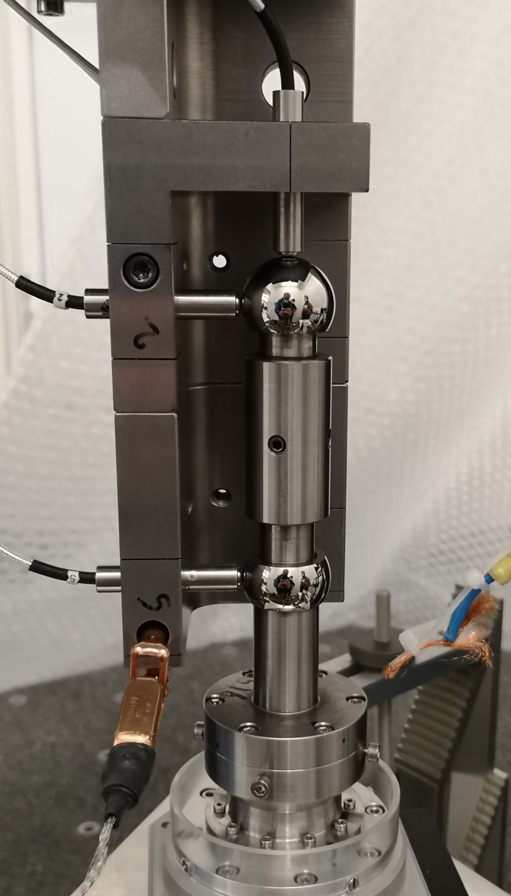
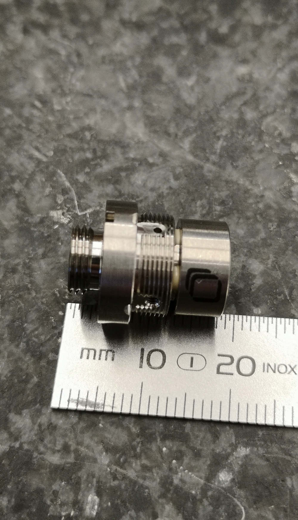
Instead of using capacitive sensors, 5 fibered interferometers were used in a similar way (Figure ref:fig:test_id31_interf). At the end of each fiber, a sensor head2 (Figure ref:fig:test_id31_interf_head) is used, which consists of a lens precisely positioned with respect to the fiber's end. The lens is focusing the light on the surface of the sphere, such that it comes back to the fiber and produces an interference. This way, the gap between the sensor and the reference sphere is much larger (here around $40\,mm$), removing the risk of collision.
Nevertheless, the metrology system still has limited measurement range, as when the spheres are moving perpendicularly to the beam axis, the reflected light does not coincide with the incident light, and for some perpendicular displacement, the interference is too small to be detected.
Metrology Kinematics
<<ssec:test_id31_metrology_kinematics>>
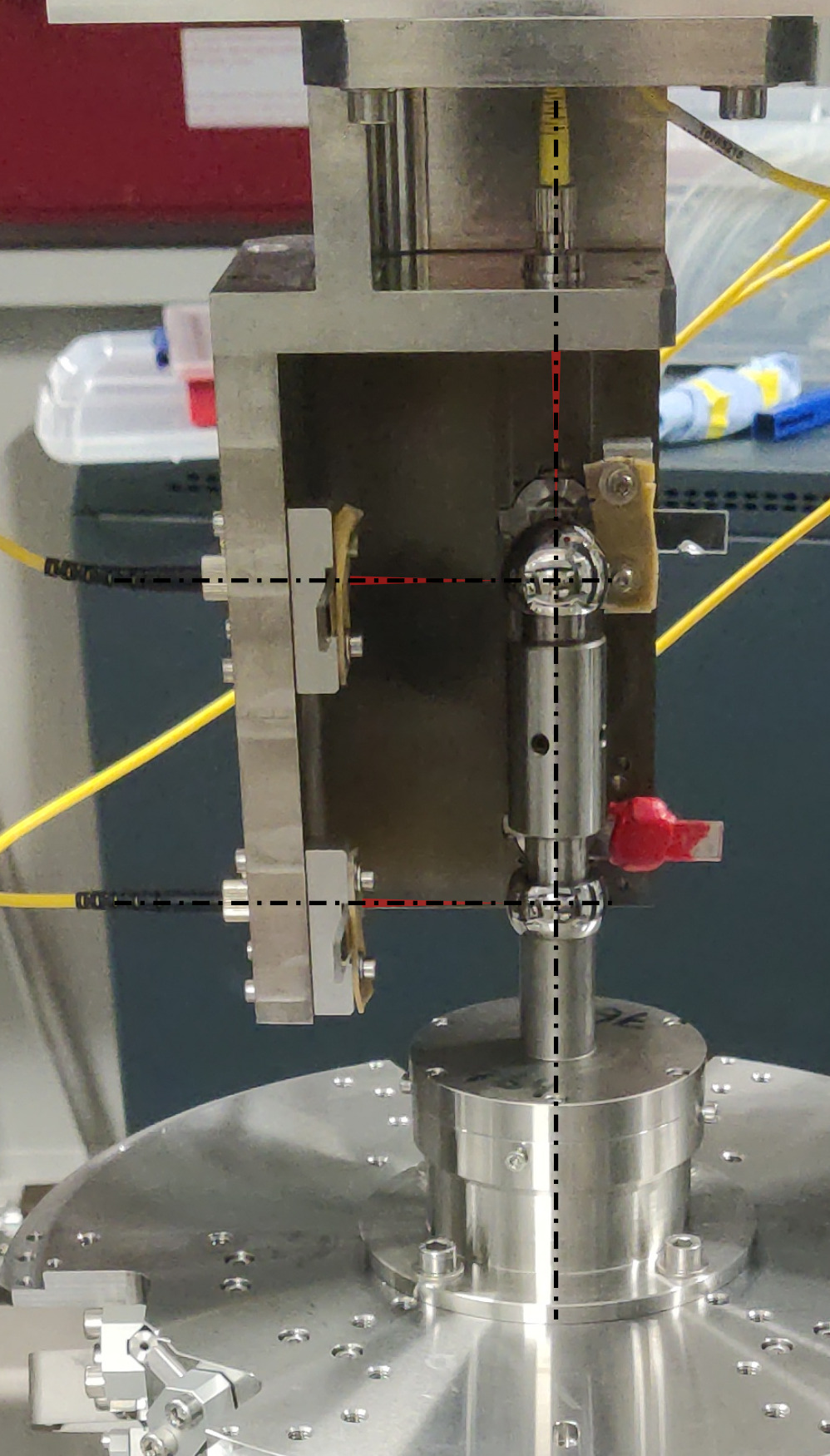
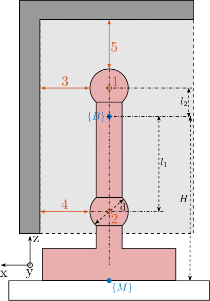
The developed short-stroke metrology system is schematically shown in Figure ref:fig:test_id31_metrology_kinematics. The point of interest is indicated by the blue frame $\{B\}$, which is located $H = 150\,mm$ above the nano-hexapod's top platform. The spheres have a diameter $d = 25.4\,mm$, and indicated dimensions are $l_1 = 60\,mm$ and $l_2 = 16.2\,mm$. In order to compute the pose of the $\{B\}$ frame with respect to the granite (i.e. with respect to the fixed interferometer heads), the measured small displacements $[d_1,\ d_2,\ d_3,\ d_4,\ d_5]$ by the interferometers are first written as a function of the small linear and angular motion of the $\{B\}$ frame $[D_x,\ D_y,\ D_z,\ R_x,\ R_y]$ eqref:eq:test_id31_metrology_kinematics.
\begin{equation}\label{eq:test_id31_metrology_kinematics} d_1 = D_y - l_2 R_x, \quad d_2 = D_y + l_1 R_x, \quad d_3 = -D_x - l_2 R_y, \quad d_4 = -D_x + l_1 R_y, \quad d_5 = -D_z
\end{equation}
\hfill
The five equations eqref:eq:test_id31_metrology_kinematics can be written in a matrix form, and then inverted to have the pose of $\{B\}$ frame as a linear combination of the measured five distances by the interferometers eqref:eq:test_id31_metrology_kinematics_inverse.
\begin{equation}\label{eq:test_id31_metrology_kinematics_inverse}
\begin{bmatrix} D_x \\ D_y \\ D_z \\ R_x \\ R_y \end{bmatrix} = \begin{bmatrix} 0 & 1 & 0 & -l_2 & 0 \\ 0 & 1 & 0 & l_1 & 0 \\ -1 & 0 & 0 & 0 & -l_2 \\ -1 & 0 & 0 & 0 & l_1 \\ 0 & 0 & -1 & 0 & 0 \end{bmatrix}^{-1} \cdot \begin{bmatrix} d_1 \\ d_2 \\ d_3 \\ d_4 \\ d_5 \end{bmatrix}\end{equation}
%% Geometrical parameters of the metrology system
H = 150e-3;
l1 = (150-48-42)*1e-3;
l2 = (76.2+48+42-150)*1e-3;

% Computation of the Transformation matrix
Hm = [ 0  1  0 -l2  0;
       0  1  0  l1  0;
      -1  0  0  0  -l2;
      -1  0  0  0   l1;
       0  0 -1  0   0];
Rough alignment of the reference spheres
<<ssec:test_id31_metrology_sphere_rought_alignment>>
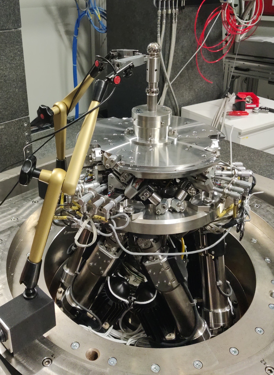
The two reference spheres are aligned with the rotation axis of the spindle. To do so, two measuring probes are used as shown in Figure ref:fig:align_top_sphere_comparators.
To not damage the sensitive sphere surface, the probes are instead positioned on the cylinder on which the sphere is mounted. First, the probes are fixed to the bottom (fixed) cylinder to align its axis with the spindle axis. Then, the probes are fixed to the top (adjustable) cylinder, and the same alignment is performed.
With this setup, the precision of the alignment of both sphere better with the spindle axis is expected to limited to $\approx 10\,\mu m$. This is probably limited due to the poor coaxiality between the cylinders and the spheres. However, the alignment precision should be enough to stay in the acceptance of the interferometers.
Tip-Tilt adjustment of the interferometers
<<ssec:test_id31_metrology_alignment>>
The short stroke metrology system is placed on top of the main granite using a gantry made of granite blocs to have good vibration and thermal stability (Figure ref:fig:short_stroke_metrology_overview).
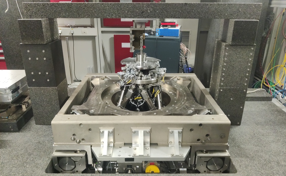
The interferometers need to be aligned with respect to the two reference spheres to approach as much as possible the ideal case shown in Figure ref:fig:test_id31_metrology_kinematics. The vertical position of the spheres is adjusted using the micro-hexapod to match the height of the interferometers. Then, the horizontal position of the gantry is adjusted such that the coupling efficiency (i.e. the intensity of the light reflected back in the fiber) of the top interferometer is maximized. This is equivalent as to optimize the perpendicularity between the interferometer beam and the sphere surface (i.e. the concentricity between the beam and the sphere center).
The lateral sensor heads (i.e. all except the top one), which are each fixed to a custom tip-tilt adjustment mechanism, are individually oriented such that the coupling efficient is maximized.
Fine Alignment of reference spheres using interferometers
<<ssec:test_id31_metrology_sphere_fine_alignment>>
Thanks to the good alignment of the two reference spheres with the spindle axis and to the fine adjustment of the interferometers orientations, the interferometer measurement is made possible during complete spindle rotation. This metrology and therefore be used to better align the axis defined by the two spheres' center with the spindle axis.
The alignment process is made by few iterations. First, the spindle is scanned and the alignment errors are recorded. From the errors, the motion of the micro-hexapod to better align the spheres is determined and the micro-hexapod is moved. Then, the spindle is scanned again, and the new alignment errors are recorded.
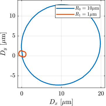
This iterative process is first perform for angular errors (Figure ref:fig:test_id31_metrology_align_rx_ry) and then for lateral errors (Figure ref:fig:test_id31_metrology_align_dx_dy). Remaining error after alignment is in the order of $\pm5\,\mu\text{rad}$ for angular errors, $\pm 1\,\mu m$ laterally and less than $0.1\,\mu m$ vertically.
%% Angular alignment
% Load Data
data_it0 = h5scan(data_dir, 'alignment', 'h1rx_h1ry', 1);
data_it1 = h5scan(data_dir, 'alignment', 'h1rx_h1ry_0002', 3);
data_it2 = h5scan(data_dir, 'alignment', 'h1rx_h1ry_0002', 5);

% Offset wrong points
i_it0 = find(abs(data_it0.Rx_int_filtered(2:end)-data_it0.Rx_int_filtered(1:end-1))>1e-5);
data_it0.Rx_int_filtered(i_it0+1:end) = data_it0.Rx_int_filtered(i_it0+1:end) + data_it0.Rx_int_filtered(i_it0) - data_it0.Rx_int_filtered(i_it0+1);
i_it1 = find(abs(data_it1.Rx_int_filtered(2:end)-data_it1.Rx_int_filtered(1:end-1))>1e-5);
data_it1.Rx_int_filtered(i_it1+1:end) = data_it1.Rx_int_filtered(i_it1+1:end) + data_it1.Rx_int_filtered(i_it1) - data_it1.Rx_int_filtered(i_it1+1);
i_it2 = find(abs(data_it2.Rx_int_filtered(2:end)-data_it2.Rx_int_filtered(1:end-1))>1e-5);
data_it2.Rx_int_filtered(i_it2+1:end) = data_it2.Rx_int_filtered(i_it2+1:end) + data_it2.Rx_int_filtered(i_it2) - data_it2.Rx_int_filtered(i_it2+1);

% Compute circle fit and get radius
[~, ~, R_it0, ~] = circlefit(1e6*data_it0.Rx_int_filtered, 1e6*data_it0.Ry_int_filtered);
[~, ~, R_it1, ~] = circlefit(1e6*data_it1.Rx_int_filtered, 1e6*data_it1.Ry_int_filtered);
[~, ~, R_it2, ~] = circlefit(1e6*data_it2.Rx_int_filtered, 1e6*data_it2.Ry_int_filtered);
%% Eccentricity alignment
% Load Data
data_it0 = h5scan(data_dir, 'alignment', 'h1rx_h1ry_0002', 5);
data_it1 = h5scan(data_dir, 'alignment', 'h1dx_h1dy', 1);
% Offset wrong points
i_it0 = find(abs(data_it0.Dy_int_filtered(2:end)-data_it0.Dy_int_filtered(1:end-1))>1e-5);
data_it0.Dy_int_filtered(i_it0+1:end) = data_it0.Dy_int_filtered(i_it0+1:end) + data_it0.Dy_int_filtered(i_it0) - data_it0.Dy_int_filtered(i_it0+1);
% Compute circle fit and get radius
[~, ~, R_it0, ~] = circlefit(1e6*data_it0.Dx_int_filtered, 1e6*data_it0.Dy_int_filtered);
[~, ~, R_it1, ~] = circlefit(1e6*data_it1.Dx_int_filtered, 1e6*data_it1.Dy_int_filtered);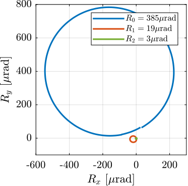
Estimated measurement volume
<<ssec:test_id31_metrology_acceptance>>
Because the interferometers are pointing to spheres and not flat surfaces, the lateral acceptance is limited. In order to estimate the metrology acceptance, the micro-hexapod is used to perform three accurate scans of $\pm 1\,mm$, respectively along the the $x$, $y$ and $z$ axes. During these scans, the 5 interferometers are recorded, and the ranges in which each interferometer has enough coupling efficiency for measurement are estimated. Results are summarized in Table ref:tab:test_id31_metrology_acceptance. The obtained lateral acceptance for pure displacements in any direction is estimated to be around $+/-0.5\,mm$, which is enough for the current application as it is well above the micro-station errors to be actively corrected.
%% Estimated acceptance of the metrology
% This is estimated by moving the spheres using the micro-hexapod

% Dx
data_dx = h5scan(data_dir, 'metrology_acceptance_new_align', 'dx', 1);

dx_acceptance = zeros(5,1);

for i = [1:size(dx_acceptance, 1)]
    % Find range in which the interferometers are measuring displacement
    dx_di = diff(data_dx.(sprintf('d%i', i))) == 0;
    if sum(dx_di) > 0
        dx_acceptance(i) = data_dx.h1tx(find(dx_di(501:end), 1) + 500) - ...
                           data_dx.h1tx(find(flip(dx_di(1:500)), 1));
    else
        dx_acceptance(i) = data_dx.h1tx(end) - data_dx.h1tx(1);
    end
end

% Dy
data_dy = h5scan(data_dir, 'metrology_acceptance_new_align', 'dy', 1);

dy_acceptance = zeros(5,1);

for i = [1:size(dy_acceptance, 1)]
    % Find range in which the interferometers are measuring displacement
    dy_di = diff(data_dy.(sprintf('d%i', i))) == 0;
    if sum(dy_di) > 0
        dy_acceptance(i) = data_dy.h1ty(find(dy_di(501:end), 1) + 500) - ...
                           data_dy.h1ty(find(flip(dy_di(1:500)), 1));
    else
        dy_acceptance(i) = data_dy.h1ty(end) - data_dy.h1ty(1);
    end
end

% Dz
data_dz = h5scan(data_dir, 'metrology_acceptance_new_align', 'dz', 1);

dz_acceptance = zeros(5,1);

for i = [1:size(dz_acceptance, 1)]
    % Find range in which the interferometers are measuring displacement
    dz_di = diff(data_dz.(sprintf('d%i', i))) == 0;
    if sum(dz_di) > 0
        dz_acceptance(i) = data_dz.h1tz(find(dz_di(501:end), 1) + 500) - ...
                           data_dz.h1tz(find(flip(dz_di(1:500)), 1));
    else
        dz_acceptance(i) = data_dz.h1tz(end) - data_dz.h1tz(1);
    end
end| $D_x$ | $D_y$ | $D_z$ | |
|---|---|---|---|
| $d_1$ (y) | $1.0\,mm$ | $>2\,mm$ | $1.35\,mm$ |
| $d_2$ (y) | $0.8\,mm$ | $>2\,mm$ | $1.01\,mm$ |
| $d_3$ (x) | $>2\,mm$ | $1.06\,mm$ | $1.38\,mm$ |
| $d_4$ (x) | $>2\,mm$ | $0.99\,mm$ | $0.94\,mm$ |
| $d_5$ (z) | $1.33\, mm$ | $1.06\,mm$ | $>2\,mm$ |
Estimated measurement errors
<<ssec:test_id31_metrology_errors>>
When using the NASS, the accuracy of the sample's positioning is linked to the accuracy of the external metrology. However, to validate the nano-hexapod with the associated instrumentation and control architecture, the accuracy of the metrology is not an issue. Only the bandwidth and noise characteristics of the external metrology are important. Yet, some elements effecting the accuracy of the metrology are discussed here.
First, the "metrology kinematics" (discussed in Section ref:ssec:test_id31_metrology_kinematics) is only approximate (i.e. valid for very small displacements). This can be seen when performing lateral $[D_x,\,D_y]$ scans using the micro-hexapod while recording the vertical interferometer (Figure ref:fig:test_id31_xy_map_sphere). As the interferometer is pointing to a sphere and not to a plane, lateral motion of the sphere is seen as a vertical motion by the top interferometer.
Then, the reference spheres have some deviations with respect to an ideal sphere. They are meant to be used with capacitive sensors which are integrating the shape errors over large surfaces. When using interferometers, the size of the "light spot" on the sphere surface is a circle with a diameter $\approx 50\,\mu m$, therefore the system is more sensitive to shape errors with small features.
As the interferometer light is travelling in air, the measured distance is sensitive to any variation in the refractive index of the air. Therefore, any variation of air temperature, pressure or humidity will induce measurement errors. For a measurement length of $40\,mm$, a temperature variation of $0.1\,{}^oC$ induces an errors in the distance measurement of $\approx 4\,nm$.
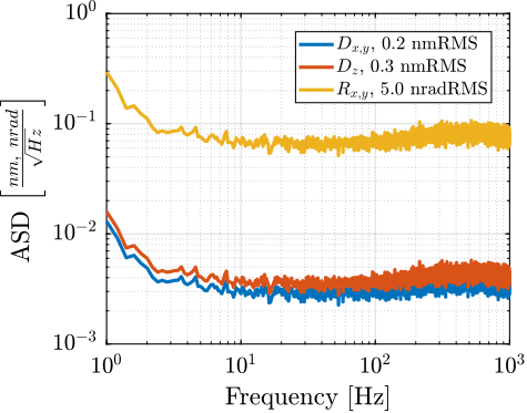
Finally, even in vacuum and in the absence of target motion, the interferometers are affected by noise cite:&watchi18_review_compac_inter. The effect of the noise on the translation and rotation measurements is estimated in Figure ref:fig:test_id31_interf_noise.
%% Interferometer noise estimation
data = load("test_id31_interf_noise.mat");

Ts = 1e-4;
Nfft = floor(5/Ts);
win = hanning(Nfft);
Noverlap = floor(Nfft/2);

[pxx_int, f] = pwelch(detrend(data.d, 0), win, Noverlap, Nfft, 1/Ts);

% Uncorrelated noise: square root of the sum of the squares
pxx_cart = pxx_int*sum(inv(Hm).^2, 2)';

rms_dxy = sqrt(trapz(f(f>1), pxx_cart((f>1),1))); % < 0.3 nm RMS
rms_dz  = sqrt(trapz(f(f>1), pxx_cart((f>1),3))); % < 0.3 nm RMS
rms_rxy = sqrt(trapz(f(f>1), pxx_cart((f>1),4))); % 5 nrad RMSfigure;
hold on;
plot(f, sqrt(pxx_cart(:,1)), 'DisplayName', sprintf('$D_{x,y}$, %.1f nmRMS', rms_dxy));
plot(f, sqrt(pxx_cart(:,3)), 'DisplayName', sprintf('$D_{z}$, %.1f nmRMS', rms_dz));
plot(f, sqrt(pxx_cart(:,4)), 'DisplayName', sprintf('$R_{x,y}$, %.1f nradRMS', rms_rxy));
set(gca, 'xscale', 'log'); set(gca, 'yscale', 'log');
xlabel('Frequency [Hz]'); ylabel('ASD $\left[\frac{nm,\ nrad}{\sqrt{Hz}}\right]$')
xlim([1, 1e3]); ylim([1e-3, 1]);
leg = legend('location', 'northeast', 'FontSize', 8, 'NumColumns', 1);
leg.ItemTokenSize(1) = 15;%% X-Y scan with the micro-hexapod, and record of the vertical interferometer
data = h5scan(data_dir, 'metrology_acceptance', 'after_int_align_meshXY', 1);
x = 1e3*detrend(data.h1tx, 0); % [um]
y = 1e3*detrend(data.h1ty, 0); % [um]
z = 1e6*data.Dz_int_filtered - max(data.Dz_int_filtered); % [um]
mdl = scatteredInterpolant(x, y, z);
[xg, yg] = meshgrid(unique(x), unique(y));
zg = mdl(xg, yg);
% Fit a sphere to the data
[sphere_center,sphere_radius] = sphereFit(1e-3*[x, y, z]);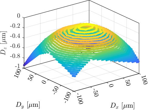
Identified Open Loop Plant
<<sec:test_id31_open_loop_plant>>
Introduction ignore
First Open-Loop Plant Identification
<<ssec:test_id31_open_loop_plant_first_id>>
The plant dynamics is first identified for a fixed spindle angle (at $0\,\text{deg}$) and without any payload. The model dynamics is also identified in the same conditions.
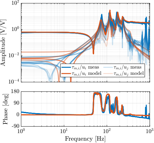
A first comparison between the model and the measured dynamics is done in Figure ref:fig:test_id31_first_id. A good match can be observed for the diagonal dynamics (except the high frequency modes which are not modeled). However, the coupling for the transfer function from command signals $\mathbf{u}$ to estimated strut motion from the external metrology $e\mathbf{\mathcal{L}}$ is larger than expected (Figure ref:fig:test_id31_first_id_int).
%% Identify the plant dynamics using the Simscape model

% Initialize each Simscape model elements
initializeGround();
initializeGranite();
initializeTy();
initializeRy();
initializeRz();
initializeMicroHexapod();
initializeNanoHexapod('flex_bot_type', '2dof', ...
                      'flex_top_type', '3dof', ...
                      'motion_sensor_type', 'plates', ...
                      'actuator_type', '2dof');
initializeSample('type', '0');

initializeSimscapeConfiguration('gravity', false);
initializeDisturbances('enable', false);
initializeLoggingConfiguration('log', 'none');
initializeController('type', 'open-loop');
initializeReferences();

% Input/Output definition
clear io; io_i = 1;
io(io_i) = linio([mdl, '/Controller'],     1, 'openinput');               io_i = io_i + 1; % Actuator Inputs
io(io_i) = linio([mdl, '/Micro-Station'],  3, 'openoutput', [], 'Fnlm');  io_i = io_i + 1; % Force Sensors
io(io_i) = linio([mdl, '/Tracking Error'], 1, 'openoutput', [], 'EdL');   io_i = io_i + 1; % Position Errors

% With no payload
Gm = linearize(mdl, io);
Gm.InputName  = {'u1', 'u2', 'u3', 'u4', 'u5', 'u6'};
Gm.OutputName = {'Fn1', 'Fn2', 'Fn3', 'Fn4', 'Fn5', 'Fn6', ...
                 'eL1', 'eL2', 'eL3', 'eL4', 'eL5', 'eL6'};
%% Identify the plant from experimental data
% Load identification data
data = load('2023-08-08_16-17_ol_plant_m0_Wz0.mat');
% Sampling Time [s]
Ts = 1e-4;
% Hannning Windows
Nfft = floor(2.0/Ts);
win = hanning(Nfft);
Noverlap = floor(Nfft/2);
% And we get the frequency vector
[~, f] = tfestimate(data.uL1.id_plant, data.uL1.e_L1, win, Noverlap, Nfft, 1/Ts);
% IFF Plant (transfer function from u to taum)
G_iff = zeros(length(f), 6, 6);
for i_strut = 1:6
eL = [data.(sprintf("uL%i", i_strut)).Vs1 ; data.(sprintf("uL%i", i_strut)).Vs2 ; data.(sprintf("uL%i", i_strut)).Vs3 ; data.(sprintf("uL%i", i_strut)).Vs4 ; data.(sprintf("uL%i", i_strut)).Vs5 ; data.(sprintf("uL%i", i_strut)).Vs6]';
G_iff(:,:,i_strut) = tfestimate(data.(sprintf("uL%i", i_strut)).id_plant, eL, win, Noverlap, Nfft, 1/Ts);
end
% INT Plant (transfer function from u to eL)
G_int = zeros(length(f), 6, 6);
for i_strut = 1:6
eL = [data.(sprintf("uL%i", i_strut)).e_L1 ; data.(sprintf("uL%i", i_strut)).e_L2 ; data.(sprintf("uL%i", i_strut)).e_L3 ; data.(sprintf("uL%i", i_strut)).e_L4 ; data.(sprintf("uL%i", i_strut)).e_L5 ; data.(sprintf("uL%i", i_strut)).e_L6]';
G_int(:,:,i_strut) = tfestimate(data.(sprintf("uL%i", i_strut)).id_plant, eL, win, Noverlap, Nfft, 1/Ts);
end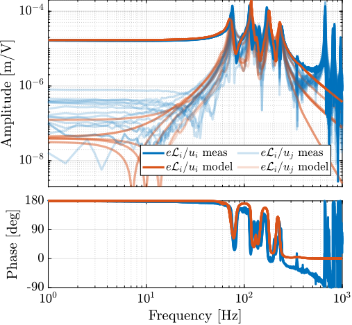
Better Angular Alignment
<<ssec:test_id31_open_loop_plant_rz_alignment>>
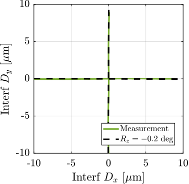
One possible explanation of the increased coupling observed in Figure ref:fig:test_id31_first_id_int is the poor alignment between the external metrology axes (i.e. the interferometer supports) and the nano-hexapod axes. To estimate this alignment, a decentralized low-bandwidth feedback controller based on the nano-hexapod encoders is implemented. This allowed to perform two straight movements of the nano-hexapod along the $x$ and $y$ axes in the frame of the nano-hexapod. During these two movements, the external metrology measurement is recorded and shown in Figure ref:fig:test_id31_Rz_align_error. It was found that there is a misalignment of 2.7 degrees (rotation along the vertical axis) between the interferometer axes and nano-hexapod axes. This was corrected by adding an offset to the spindle angle. To check that the alignment has improved, the same movement was performed using the nano-hexapod while recording the signal of the external metrology. Results shown in Figure ref:fig:test_id31_Rz_align_correct are indeed indicating much better alignment.
%% Load Data
data_1_dx = h5scan(data_dir, 'align_int_enc_Rz', 'tx_first_scan', 2);
data_1_dy = h5scan(data_dir, 'align_int_enc_Rz', 'tx_first_scan', 3);
data_2_dx = h5scan(data_dir, 'align_int_enc_Rz', 'verif-after-correct-offset', 1);
data_2_dy = h5scan(data_dir, 'align_int_enc_Rz', 'verif-after-correct-offset', 2);
% Estimation of Rz misalignment
p1 = polyfit(data_1_dx.Dx_int_filtered, data_1_dx.Dy_int_filtered, 1);
p2 = polyfit(data_1_dy.Dx_int_filtered, data_1_dy.Dy_int_filtered, 1);
Rz_error = (atan(p1(1)) + atan(p2(1))-pi/2)/2; % ~3 degrees%% Estimation of the Rz misalignment
figure;
hold on;
plot(1e6*data_1_dx.Dx_int_filtered, 1e6*data_1_dx.Dy_int_filtered, 'color', colors(2,:), 'DisplayName', 'Measurement')
plot(1e6*data_1_dy.Dx_int_filtered, 1e6*data_1_dy.Dy_int_filtered, 'color', colors(2,:), 'HandleVisibility', 'off')
plot( 1e6*[-10:10]*cos(Rz_error), 1e6*[-10:10]*sin(Rz_error), 'k--', 'DisplayName', sprintf('$R_z = %.1f$ deg', Rz_error*180/pi))
plot(-1e6*[-10:10]*sin(Rz_error), 1e6*[-10:10]*cos(Rz_error), 'k--', 'HandleVisibility', 'off')
hold off;
xlabel('Interf $D_x$ [$\mu$m]');
ylabel('Interf $D_y$ [$\mu$m]');
axis equal
xlim([-10, 10]); ylim([-10, 10]);
xticks([-10:5:10]); yticks([-10:5:10]);
leg = legend('location', 'southeast', 'FontSize', 8, 'NumColumns', 1);
leg.ItemTokenSize(1) = 15;% Estimation of Rz misalignment after correcting the Rz angle
p1 = polyfit(data_2_dx.Dx_int_filtered, data_2_dx.Dy_int_filtered, 1);
p2 = polyfit(data_2_dy.Dx_int_filtered, data_2_dy.Dy_int_filtered, 1);
Rz_error = (atan(p1(1)) + atan(p2(1))-pi/2)/2; % ~0.2 degrees%% Estimation of the Rz misalignment after correcting the Rz offset
figure;
hold on;
plot(1e6*data_2_dx.Dx_int_filtered, 1e6*data_2_dx.Dy_int_filtered, 'color', colors(5,:), 'DisplayName', 'Measurement')
plot(1e6*data_2_dy.Dx_int_filtered, 1e6*data_2_dy.Dy_int_filtered, 'color', colors(5,:), 'HandleVisibility', 'off')
plot( 1e6*[-10:10]*cos(Rz_error), 1e6*[-10:10]*sin(Rz_error), 'k--', 'DisplayName', sprintf('$R_z = %.1f$ deg', Rz_error*180/pi))
plot(-1e6*[-10:10]*sin(Rz_error), 1e6*[-10:10]*cos(Rz_error), 'k--', 'HandleVisibility', 'off')
hold off;
xlabel('Interf $D_x$ [$\mu$m]');
ylabel('Interf $D_y$ [$\mu$m]');
axis equal
xlim([-10, 10]); ylim([-10, 10]);
xticks([-10:5:10]); yticks([-10:5:10]);
leg = legend('location', 'southeast', 'FontSize', 8, 'NumColumns', 1);
leg.ItemTokenSize(1) = 15;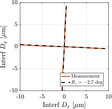
Open-Loop Identification after alignment
<<ssec:test_id31_open_loop_plant_after_alignment>>
The plant dynamics is identified after the fine alignment and is compared with the model dynamics in Figure ref:fig:test_id31_first_id_int_better_rz_align. Compared to the initial identification shown in Figure ref:fig:test_id31_first_id_int, the obtained coupling has decreased and is close to the coupling obtained with the multi-body model.
%% Identification of the plant after Rz alignment
data_align = load('2023-08-17_17-37_ol_plant_m0_Wz0_new_Rz_align.mat');

G_int_align = zeros(length(f), 6, 6);
for i_strut = 1:6
    eL = [data_align.(sprintf("uL%i", i_strut)).e_L1 ; data_align.(sprintf("uL%i", i_strut)).e_L2 ; data_align.(sprintf("uL%i", i_strut)).e_L3 ; data_align.(sprintf("uL%i", i_strut)).e_L4 ; data_align.(sprintf("uL%i", i_strut)).e_L5 ; data_align.(sprintf("uL%i", i_strut)).e_L6]';

    G_int_align(:,:,i_strut) = tfestimate(data_align.(sprintf("uL%i", i_strut)).id_plant, eL, win, Noverlap, Nfft, 1/Ts);
end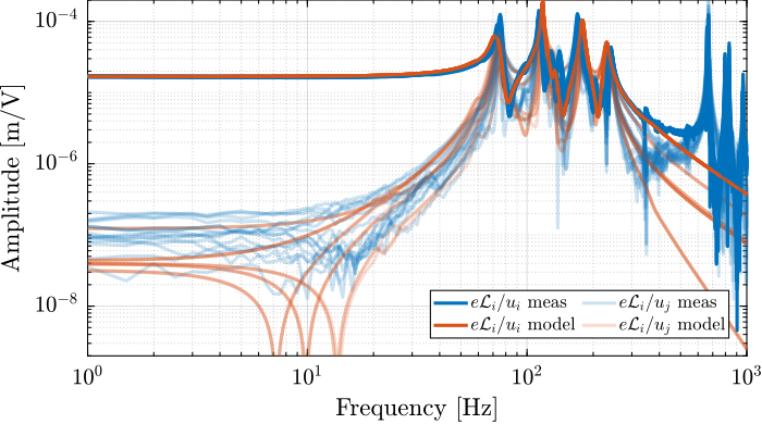
Effect of Payload Mass
<<ssec:test_id31_open_loop_plant_mass>>
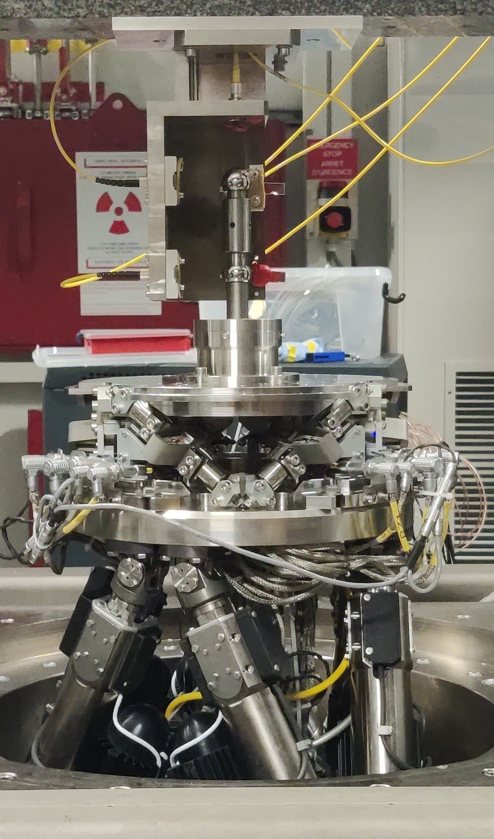
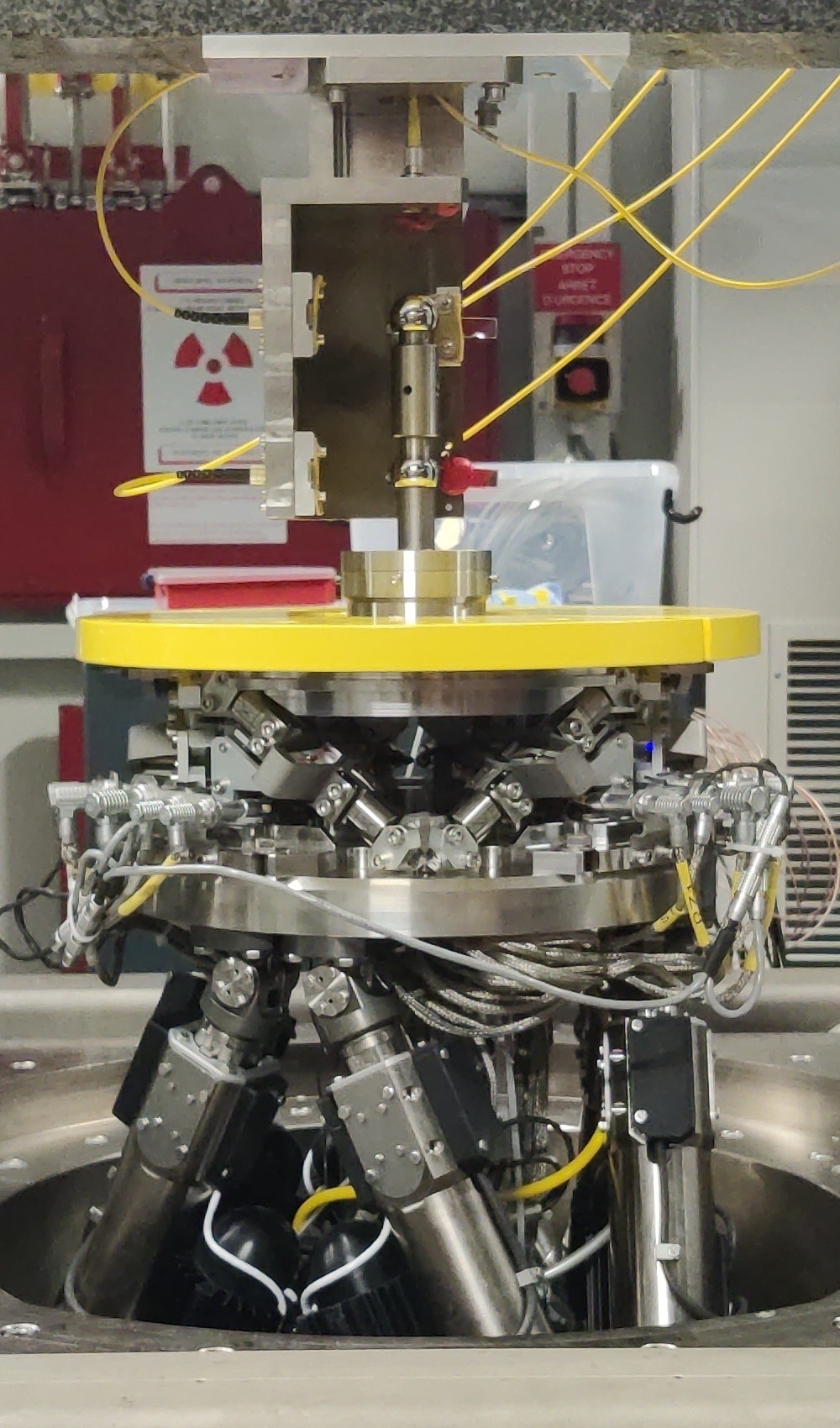
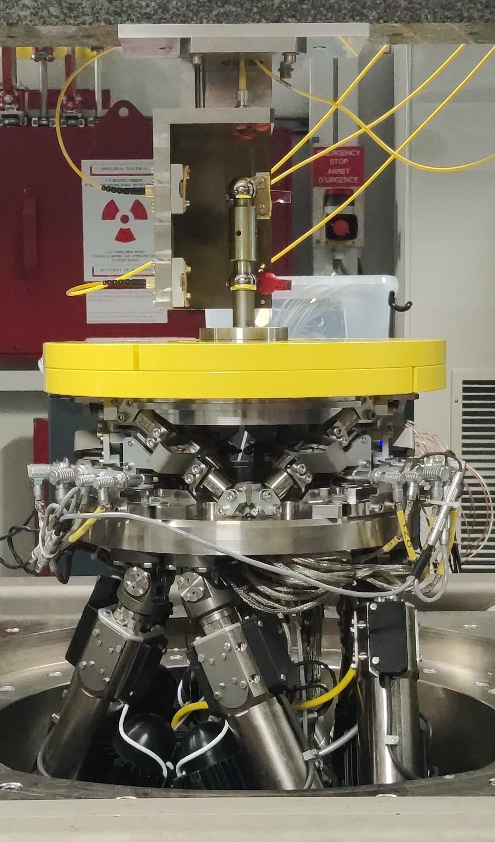
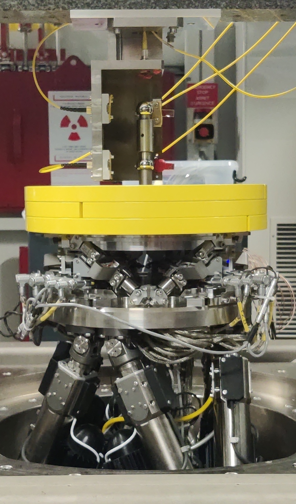
The system dynamics was identified with four payload conditions that are shown in Figure ref:fig:test_id31_picture_masses. The obtained direct terms are compared with the model dynamics in Figure ref:fig:test_nhexa_comp_simscape_diag_masses.
%% Identify the plant from experimental data - All payloads

% Load identification data
data_m0_Wz0 = load('2023-08-08_16-17_ol_plant_m0_Wz0.mat');
data_m1_Wz0 = load('2023-08-08_18-57_ol_plant_m1_Wz0.mat');
data_m2_Wz0 = load('2023-08-08_17-12_ol_plant_m2_Wz0.mat');
data_m3_Wz0 = load('2023-08-08_18-20_ol_plant_m3_Wz0.mat');

% Sampling Time [s]
Ts = 1e-4;

% Hannning Windows
Nfft = floor(2.0/Ts);
win = hanning(Nfft);
Noverlap = floor(Nfft/2);

% And we get the frequency vector
[~, f] = tfestimate(data_m0_Wz0.uL1.id_plant, data_m0_Wz0.uL1.e_L1, win, Noverlap, Nfft, 1/Ts);

% No payload
G_iff_m0_Wz0 = zeros(length(f), 6, 6);
for i_strut = 1:6
    eL = [data_m0_Wz0.(sprintf("uL%i", i_strut)).Vs1 ; data_m0_Wz0.(sprintf("uL%i", i_strut)).Vs2 ; data_m0_Wz0.(sprintf("uL%i", i_strut)).Vs3 ; data_m0_Wz0.(sprintf("uL%i", i_strut)).Vs4 ; data_m0_Wz0.(sprintf("uL%i", i_strut)).Vs5 ; data_m0_Wz0.(sprintf("uL%i", i_strut)).Vs6]';

    G_iff_m0_Wz0(:,:,i_strut) = tfestimate(data_m0_Wz0.(sprintf("uL%i", i_strut)).id_plant, eL, win, Noverlap, Nfft, 1/Ts);
end

G_int_m0_Wz0 = zeros(length(f), 6, 6);
for i_strut = 1:6
    eL = [data_m0_Wz0.(sprintf("uL%i", i_strut)).e_L1 ; data_m0_Wz0.(sprintf("uL%i", i_strut)).e_L2 ; data_m0_Wz0.(sprintf("uL%i", i_strut)).e_L3 ; data_m0_Wz0.(sprintf("uL%i", i_strut)).e_L4 ; data_m0_Wz0.(sprintf("uL%i", i_strut)).e_L5 ; data_m0_Wz0.(sprintf("uL%i", i_strut)).e_L6]';

    G_int_m0_Wz0(:,:,i_strut) = tfestimate(data_m0_Wz0.(sprintf("uL%i", i_strut)).id_plant, eL, win, Noverlap, Nfft, 1/Ts);
end

% 1 "payload layer"
G_iff_m1_Wz0 = zeros(length(f), 6, 6);
for i_strut = 1:6
    eL = [data_m1_Wz0.(sprintf("uL%i", i_strut)).Vs1 ; data_m1_Wz0.(sprintf("uL%i", i_strut)).Vs2 ; data_m1_Wz0.(sprintf("uL%i", i_strut)).Vs3 ; data_m1_Wz0.(sprintf("uL%i", i_strut)).Vs4 ; data_m1_Wz0.(sprintf("uL%i", i_strut)).Vs5 ; data_m1_Wz0.(sprintf("uL%i", i_strut)).Vs6]';

    G_iff_m1_Wz0(:,:,i_strut) = tfestimate(data_m1_Wz0.(sprintf("uL%i", i_strut)).id_plant, eL, win, Noverlap, Nfft, 1/Ts);
end

G_int_m1_Wz0 = zeros(length(f), 6, 6);
for i_strut = 1:6
    eL = [data_m1_Wz0.(sprintf("uL%i", i_strut)).e_L1 ; data_m1_Wz0.(sprintf("uL%i", i_strut)).e_L2 ; data_m1_Wz0.(sprintf("uL%i", i_strut)).e_L3 ; data_m1_Wz0.(sprintf("uL%i", i_strut)).e_L4 ; data_m1_Wz0.(sprintf("uL%i", i_strut)).e_L5 ; data_m1_Wz0.(sprintf("uL%i", i_strut)).e_L6]';

    G_int_m1_Wz0(:,:,i_strut) = tfestimate(data_m1_Wz0.(sprintf("uL%i", i_strut)).id_plant, eL, win, Noverlap, Nfft, 1/Ts);
end

% 2 "payload layers"
G_iff_m2_Wz0 = zeros(length(f), 6, 6);
for i_strut = 1:6
    eL = [data_m2_Wz0.(sprintf("uL%i", i_strut)).Vs1 ; data_m2_Wz0.(sprintf("uL%i", i_strut)).Vs2 ; data_m2_Wz0.(sprintf("uL%i", i_strut)).Vs3 ; data_m2_Wz0.(sprintf("uL%i", i_strut)).Vs4 ; data_m2_Wz0.(sprintf("uL%i", i_strut)).Vs5 ; data_m2_Wz0.(sprintf("uL%i", i_strut)).Vs6]';

    G_iff_m2_Wz0(:,:,i_strut) = tfestimate(data_m2_Wz0.(sprintf("uL%i", i_strut)).id_plant, eL, win, Noverlap, Nfft, 1/Ts);
end

G_int_m2_Wz0 = zeros(length(f), 6, 6);
for i_strut = 1:6
    eL = [data_m2_Wz0.(sprintf("uL%i", i_strut)).e_L1 ; data_m2_Wz0.(sprintf("uL%i", i_strut)).e_L2 ; data_m2_Wz0.(sprintf("uL%i", i_strut)).e_L3 ; data_m2_Wz0.(sprintf("uL%i", i_strut)).e_L4 ; data_m2_Wz0.(sprintf("uL%i", i_strut)).e_L5 ; data_m2_Wz0.(sprintf("uL%i", i_strut)).e_L6]';

    G_int_m2_Wz0(:,:,i_strut) = tfestimate(data_m2_Wz0.(sprintf("uL%i", i_strut)).id_plant, eL, win, Noverlap, Nfft, 1/Ts);
end

% 3 "payload layers"
G_iff_m3_Wz0 = zeros(length(f), 6, 6);
for i_strut = 1:6
    eL = [data_m3_Wz0.(sprintf("uL%i", i_strut)).Vs1 ; data_m3_Wz0.(sprintf("uL%i", i_strut)).Vs2 ; data_m3_Wz0.(sprintf("uL%i", i_strut)).Vs3 ; data_m3_Wz0.(sprintf("uL%i", i_strut)).Vs4 ; data_m3_Wz0.(sprintf("uL%i", i_strut)).Vs5 ; data_m3_Wz0.(sprintf("uL%i", i_strut)).Vs6]';

    G_iff_m3_Wz0(:,:,i_strut) = tfestimate(data_m3_Wz0.(sprintf("uL%i", i_strut)).id_plant, eL, win, Noverlap, Nfft, 1/Ts);
end

G_int_m3_Wz0 = zeros(length(f), 6, 6);
for i_strut = 1:6
    eL = [data_m3_Wz0.(sprintf("uL%i", i_strut)).e_L1 ; data_m3_Wz0.(sprintf("uL%i", i_strut)).e_L2 ; data_m3_Wz0.(sprintf("uL%i", i_strut)).e_L3 ; data_m3_Wz0.(sprintf("uL%i", i_strut)).e_L4 ; data_m3_Wz0.(sprintf("uL%i", i_strut)).e_L5 ; data_m3_Wz0.(sprintf("uL%i", i_strut)).e_L6]';

    G_int_m3_Wz0(:,:,i_strut) = tfestimate(data_m3_Wz0.(sprintf("uL%i", i_strut)).id_plant, eL, win, Noverlap, Nfft, 1/Ts);
end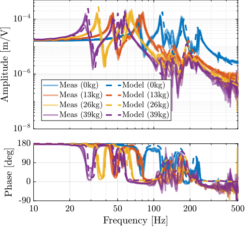
Effect of Spindle Rotation
<<ssec:test_id31_open_loop_plant_rotation>>
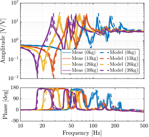
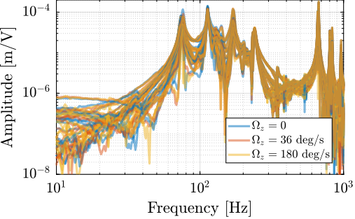
The dynamics was then identified while the Spindle was rotating at constant velocity. Three identification experiments were performed: no spindle rotation, spindle rotation at $36\,\text{deg}/s$ and at $180\,\text{deg}/s$.
The comparison of the obtained dynamics from command signal $u$ to estimated strut error $e\mathcal{L}$ is done in Figure ref:fig:test_id31_effect_rotation. Both direct terms (Figure ref:fig:test_id31_effect_rotation_direct) and coupling terms (Figure ref:fig:test_id31_effect_rotation_coupling) are unaffected by the rotation. The same can be observed for the dynamics from the command signal to the encoders and to the force sensors. This confirms that the rotation has no significant effect on the plant dynamics. This also indicates that the metrology kinematics is correct and is working in real time.
%% Identify the model dynamics with Spindle rotation
initializeSample('type', '0');
initializeReferences(...
    'Rz_type', 'rotating', ...
    'Rz_period', 360/36);
Gm_m0_Wz36 = linearize(mdl, io, 0.1);
Gm_m0_Wz36.InputName  = {'u1', 'u2', 'u3', 'u4', 'u5', 'u6'};
Gm_m0_Wz36.OutputName = {'Fn1', 'Fn2', 'Fn3', 'Fn4', 'Fn5', 'Fn6', ...
                         'eL1', 'eL2', 'eL3', 'eL4', 'eL5', 'eL6'};

initializeReferences(...
    'Rz_type', 'rotating', ...
    'Rz_period', 360/180);
Gm_m0_Wz180 = linearize(mdl, io, 0.1);
Gm_m0_Wz180.InputName  = {'u1', 'u2', 'u3', 'u4', 'u5', 'u6'};
Gm_m0_Wz180.OutputName = {'Fn1', 'Fn2', 'Fn3', 'Fn4', 'Fn5', 'Fn6', ...
                          'eL1', 'eL2', 'eL3', 'eL4', 'eL5', 'eL6'};
% The identified dynamics are then saved for further use.
save('./mat/test_id31_simscape_open_loop_plants.mat', 'Gm_m0_Wz0', 'Gm_m0_Wz180', 'Gm_m1_Wz0', 'Gm_m2_Wz0', 'Gm_m3_Wz0');%% Identify the plant from experimental data - Effect of rotation
% Load identification data
data_m0_Wz36 = load('2023-08-08_16-28_ol_plant_m0_Wz36.mat');
data_m0_Wz180 = load('2023-08-08_16-45_ol_plant_m0_Wz180.mat');
% Spindle Rotation at 36 deg/s
G_iff_m0_Wz36 = zeros(length(f), 6, 6);
for i_strut = 1:6
eL = [data_m0_Wz36.(sprintf("uL%i", i_strut)).Vs1 ; data_m0_Wz36.(sprintf("uL%i", i_strut)).Vs2 ; data_m0_Wz36.(sprintf("uL%i", i_strut)).Vs3 ; data_m0_Wz36.(sprintf("uL%i", i_strut)).Vs4 ; data_m0_Wz36.(sprintf("uL%i", i_strut)).Vs5 ; data_m0_Wz36.(sprintf("uL%i", i_strut)).Vs6]';
G_iff_m0_Wz36(:,:,i_strut) = tfestimate(data_m0_Wz36.(sprintf("uL%i", i_strut)).id_plant, eL, win, Noverlap, Nfft, 1/Ts);
end
G_int_m0_Wz36 = zeros(length(f), 6, 6);
for i_strut = 1:6
eL = [data_m0_Wz36.(sprintf("uL%i", i_strut)).e_L1 ; data_m0_Wz36.(sprintf("uL%i", i_strut)).e_L2 ; data_m0_Wz36.(sprintf("uL%i", i_strut)).e_L3 ; data_m0_Wz36.(sprintf("uL%i", i_strut)).e_L4 ; data_m0_Wz36.(sprintf("uL%i", i_strut)).e_L5 ; data_m0_Wz36.(sprintf("uL%i", i_strut)).e_L6]';
G_int_m0_Wz36(:,:,i_strut) = tfestimate(data_m0_Wz36.(sprintf("uL%i", i_strut)).id_plant, eL, win, Noverlap, Nfft, 1/Ts);
end
% Spindle Rotation at 180 deg/s
G_iff_m0_Wz180 = zeros(length(f), 6, 6);
for i_strut = 1:6
eL = [data_m0_Wz180.(sprintf("uL%i", i_strut)).Vs1 ; data_m0_Wz180.(sprintf("uL%i", i_strut)).Vs2 ; data_m0_Wz180.(sprintf("uL%i", i_strut)).Vs3 ; data_m0_Wz180.(sprintf("uL%i", i_strut)).Vs4 ; data_m0_Wz180.(sprintf("uL%i", i_strut)).Vs5 ; data_m0_Wz180.(sprintf("uL%i", i_strut)).Vs6]';
G_iff_m0_Wz180(:,:,i_strut) = tfestimate(data_m0_Wz180.(sprintf("uL%i", i_strut)).id_plant, eL, win, Noverlap, Nfft, 1/Ts);
end
G_int_m0_Wz180 = zeros(length(f), 6, 6);
for i_strut = 1:6
eL = [data_m0_Wz180.(sprintf("uL%i", i_strut)).e_L1 ; data_m0_Wz180.(sprintf("uL%i", i_strut)).e_L2 ; data_m0_Wz180.(sprintf("uL%i", i_strut)).e_L3 ; data_m0_Wz180.(sprintf("uL%i", i_strut)).e_L4 ; data_m0_Wz180.(sprintf("uL%i", i_strut)).e_L5 ; data_m0_Wz180.(sprintf("uL%i", i_strut)).e_L6]';
G_int_m0_Wz180(:,:,i_strut) = tfestimate(data_m0_Wz180.(sprintf("uL%i", i_strut)).id_plant, eL, win, Noverlap, Nfft, 1/Ts);
end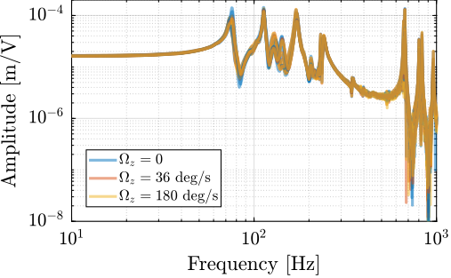
Conclusion
Thanks to the model, poor alignment between the nano-hexapod axes and the external metrology axes could be identified. After alignment, the identified dynamics is well matching with the multi-body model.
Also, the effects of the payload mass and of the spindle rotation are well capture in the model.
Decentralized Integral Force Feedback
<<sec:test_id31_iff>>
Introduction ignore
IFF Plants
Introduction ignore
6x6 Plant
%% Load identification data
data = load(sprintf('%s/dynamics/2023-08-08_16-17_ol_plant_m0_Wz0.mat', mat_dir));
Compare with Model:
load('Gm_iff.mat');Effect of Rotation
%% Load identification data
data_Wz0 = load(sprintf('%s/dynamics/2023-08-08_16-17_ol_plant_m0_Wz0.mat', mat_dir));
data_Wz1 = load(sprintf('%s/dynamics/2023-08-08_16-28_ol_plant_m0_Wz36.mat', mat_dir));
data_Wz2 = load(sprintf('%s/dynamics/2023-08-08_16-45_ol_plant_m0_Wz180.mat', mat_dir));
Effect of Mass
load('G_ol.mat', 'G_iff_m0', 'G_iff_m1', 'G_iff_m2', 'G_iff_m3', 'f');
Compare with the model
load('Gm.mat')
IFF Controller
Controller Design
Test second order high pass filter:
wz = 2*pi*10;
xiz = 0.7;
Ghpf = (s^2/wz^2)/(s^2/wz^2 + 2*xiz*s/wz + 1)
       % s/(2*pi*1)/(1 + s/(2*pi*1)) * ... % HPF: reduce gain at low frequency
We want integral action between 20Hz and 200Hz.
%% IFF Controller
Kiff = -1e2 * ...                           % Gain
       1/(0.01*2*pi + s) * ...               % LPF: provides integral action
       Ghpf * ...
       eye(6);                             % Diagonal 6x6 controller
Kiff.InputName = {'Fn1', 'Fn2', 'Fn3', 'Fn4', 'Fn5', 'Fn6'};
Kiff.OutputName = {'u1', 'u2', 'u3', 'u4', 'u5', 'u6'};
Loop Gain:

Root Locus to obtain optimal gain.

TODO Verify Stability
Verify Stability with Nyquist plot:
- Why bad stability margins?
Save Controller
save('./matlab/mat/K_iff.mat', 'Kiff')Estimated Damped Plant
%% Damped plant from Simscape model
Gm_hac_m0 = -feedback(Gm_m0, Kiff, 'name', +1);
Gm_hac_m1 = -feedback(Gm_m1, Kiff, 'name', +1);
Gm_hac_m2 = -feedback(Gm_m2, Kiff, 'name', +1);
Gm_hac_m3 = -feedback(Gm_m3, Kiff, 'name', +1);
%% Verify Stability
isstable(Gm_hac_m0)
isstable(Gm_hac_m1)
isstable(Gm_hac_m2)
isstable(Gm_hac_m3)%% Save Damped Plants
save('./matlab/mat/Gm.mat', 'Gm_hac_m0', 'Gm_hac_m1', 'Gm_hac_m2', 'Gm_hac_m3', '-append');