phd-test-bench-id31/test-bench-id31.org

Experimental Validation on the ID31 Beamline

• Glossary and Acronyms - Tables
• Introduction
• Short Stroke Metrology System
  • Introduction
  • Metrology Kinematics
  • Rough alignment of the reference spheres
  • Tip-Tilt adjustment of the interferometers
  • Fine Alignment of reference spheres using interferometers
  • Estimated measurement volume
  • Estimated measurement errors
• Open Loop Plant
  • Introduction
  • Open-Loop Plant Identification
  • Better Angular Alignment
  • Effect of Payload Mass
  • Effect of Spindle Rotation
  • Conclusion
• Decentralized Integral Force Feedback
  • Introduction
  • IFF Plant
  • IFF Controller
  • Damped Plant
  • Conclusion
• High Authority Control in the frame of the struts
  • Introduction
  • Damped Plant
  • Interaction Analysis
  • Robust Controller Design
  • Performance estimation with simulation of Tomography scans
  • Robustness estimation with simulation of Tomography scans
  • Conclusion
• Validation with Scientific experiments
  • Introduction
  • Tomography Scans
    • Slow Tomography scans
    • Fast Tomography scans
    • Cumulative Amplitude Spectra
  • Reflectivity Scans
  • Dirty Layer Scans
    • Introduction
    • Step by Step $D_z$ motion
    • Continuous $D_z$ motion: Dirty Layer Scans
  • Lateral Scans
    • Introduction
    • Slow scan
    • Fast Scan
  • Diffraction Tomography
  • Conclusion
• Conclusion
• Bibliography
• Footnotes

---

This report is also available as a pdf.

---

Glossary and Acronyms - Tables   ignore

key	abbreviation	full form
nass	NASS	Nano Active Stabilization System
fem	FEM	Finite Element Model
apa	APA	Amplified Piezoelectric Actuator
dac	DAC	Digital to Analog Converter
rga	RGA	Relative Gain Array

Introduction   ignore

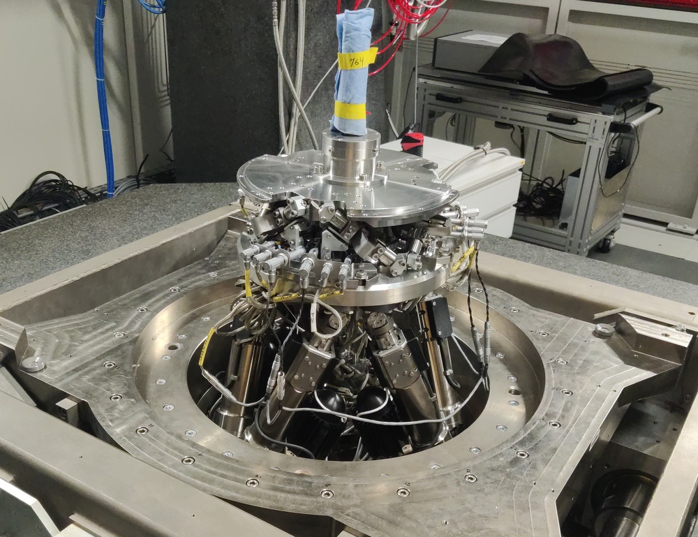
The nano-hexapod's mounting and validation through dynamics measurements marks a crucial milestone in the development of the Nano Active Stabilization System (NASS). This chapter presents a comprehensive experimental evaluation of the complete system's performance on the ID31 beamline, focusing on its ability to maintain precise sample positioning during various experimental conditions.

Initially, the project planned to develop a long-stroke ($\approx 1 \, cm^3$) 5-DoF metrology system to measure sample position relative to the granite base. However, the complexity of this development prevented its completion before the experimental testing phase on ID31. To proceed with validation of the nano active platform and its associated control architecture, an alternative short-stroke ($> 100\,\mu m^3$) metrology system was developed, which is presented in Section ref:sec:test_id31_metrology.

Then, several key aspects of the system validation are examined. Section ref:sec:test_id31_open_loop_plant analyzes the identified dynamics of the nano-hexapod mounted on the micro-station under various experimental conditions, including different payload masses and rotational velocities. These measurements are compared with predictions from the multi-body model to verify its accuracy and applicability for control design.

Sections ref:sec:test_id31_iff and ref:sec:test_id31_hac focus on the implementation and validation of the HAC-LAC control architecture. First, Section ref:sec:test_id31_iff demonstrates the application of decentralized Integral Force Feedback for robust active damping of the nano-hexapod's suspension modes. This is followed in Section ref:sec:test_id31_hac by the implementation of the high authority controller, which addresses low-frequency disturbances and completes the control system design.

Finally, Section ref:sec:test_id31_experiments evaluates the NASS's positioning performances through a comprehensive series of experiments that mirror typical scientific applications. These include tomography scans at various speeds and with different payload masses, reflectivity measurements, and combined motion sequences that test the system's full capabilities.

Short Stroke Metrology System

<<sec:test_id31_metrology>>

Introduction   ignore

The control of the nano-hexapod requires an external metrology system measuring the relative position of the nano-hexapod top platform with respect to the granite. As the long-stroke ($\approx 1 \,cm^3$) metrology system was not developed yet, a stroke stroke ($> 100\,\mu m^3$) was used instead to validate the nano-hexapod control.

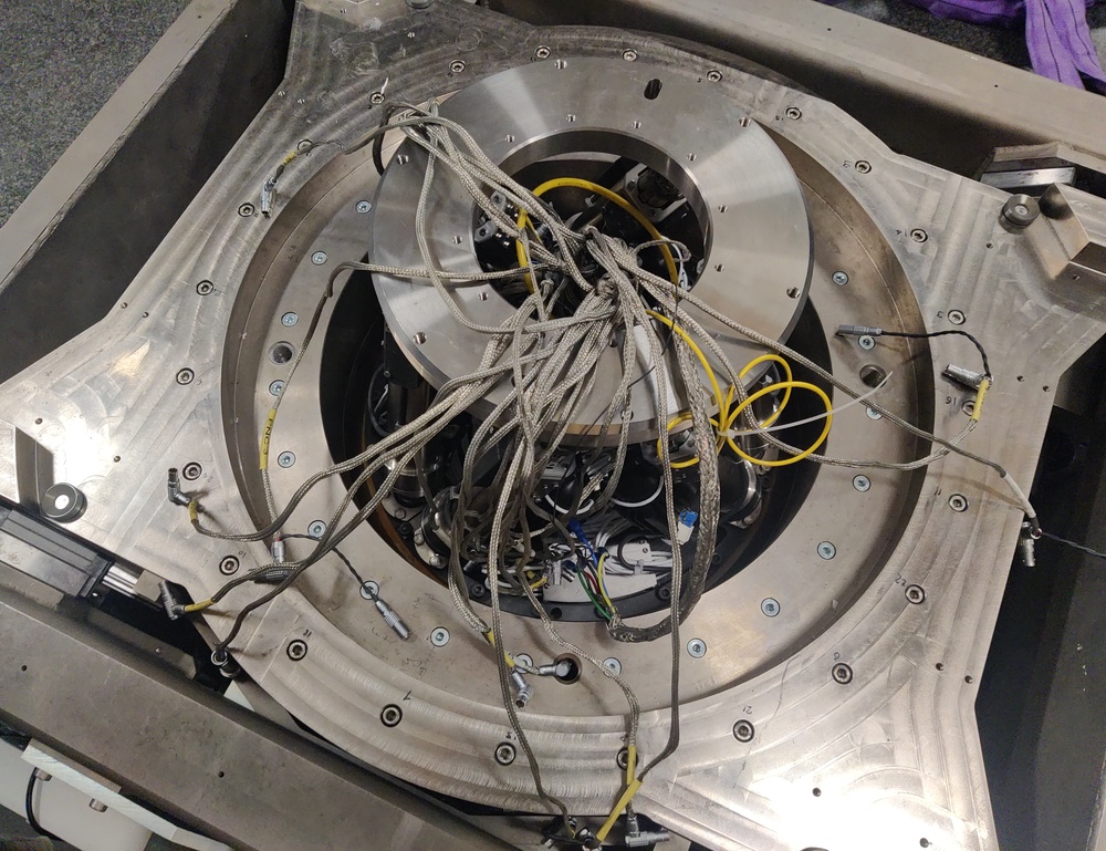
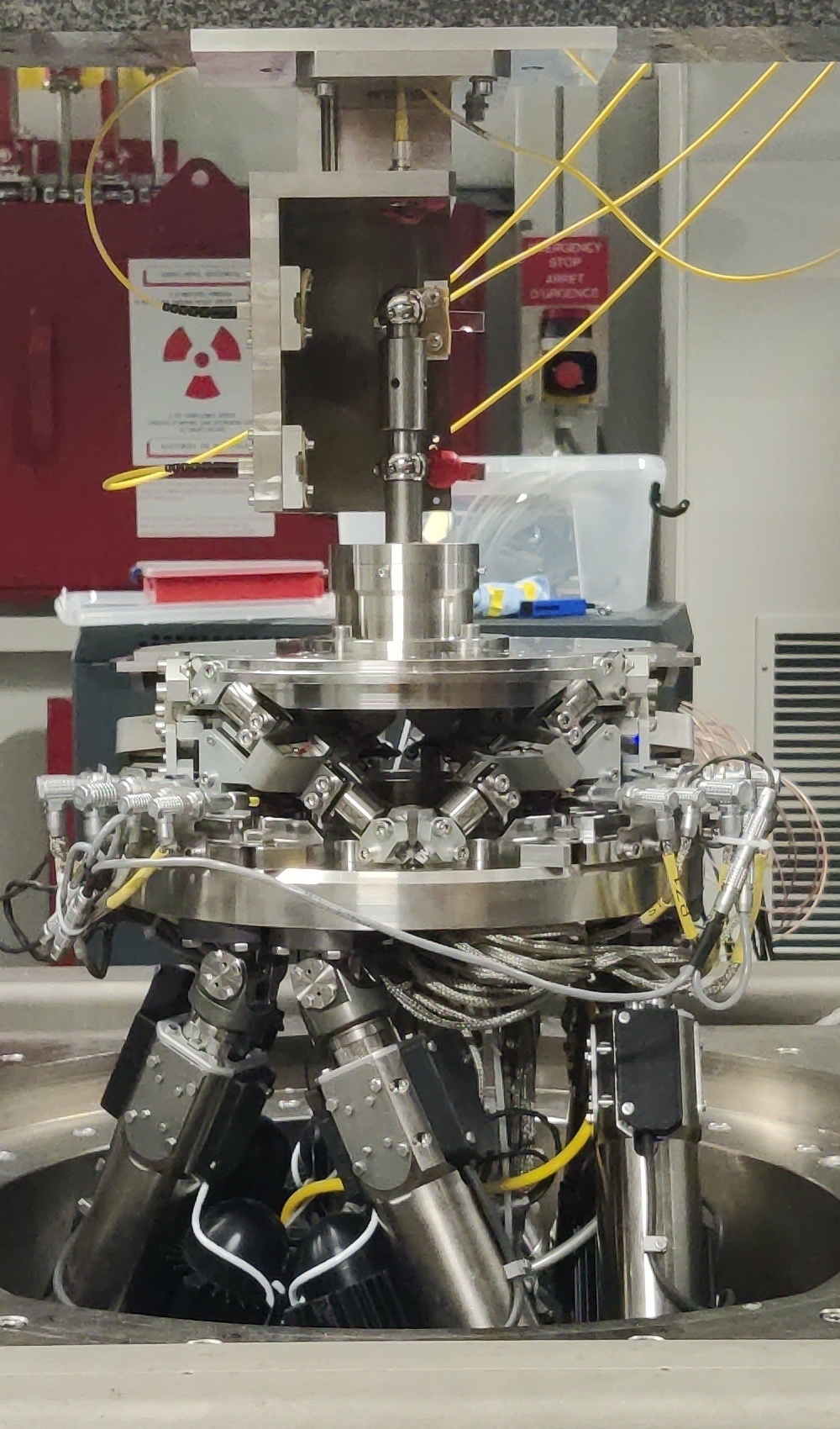
A first considered option was to use the "Spindle error analyzer" shown in Figure ref:fig:test_id31_lion. This system comprises 5 capacitive sensors which are facing two reference spheres. But as the gap between the capacitive sensors and the spheres is very small¹, the risk of damaging the spheres and the capacitive sensors is too high.

Instead of using capacitive sensors, 5 fibered interferometers were used in a similar way (Figure ref:fig:test_id31_interf). At the end of each fiber, a sensor head² (Figure ref:fig:test_id31_interf_head) is used, which consists of a lens precisely positioned with respect to the fiber's end. The lens is focusing the light on the surface of the sphere, such that the reflected light comes back into the fiber and produces an interference. This way, the gap between the head and the reference sphere is much larger (here around $40\,mm$), removing the risk of collision.

Nevertheless, the metrology system still has limited measurement range due to limited angular acceptance of the fibered interferometers. Indeed, when the spheres are moving perpendicularly to the beam axis, the reflected light does not coincide with the incident light, and above some perpendicular displacement, the reflected light does not comes back into the fiber, and no interference is produced.

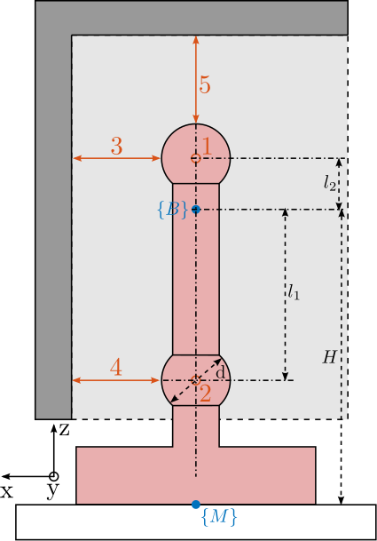
Metrology Kinematics

<<ssec:test_id31_metrology_kinematics>>

The developed short-stroke metrology system is schematically shown in Figure ref:fig:test_id31_metrology_kinematics. The point of interest is indicated by the blue frame $\{B\}$, which is located $H = 150\,mm$ above the nano-hexapod's top platform. The spheres have a diameter $d = 25.4\,mm$, and indicated dimensions are $l_1 = 60\,mm$ and $l_2 = 16.2\,mm$. In order to compute the pose of the $\{B\}$ frame with respect to the granite (i.e. with respect to the fixed interferometer heads), the measured (small) displacements $[d_1,\ d_2,\ d_3,\ d_4,\ d_5]$ by the interferometers are first written as a function of the (small) linear and angular motion of the $\{B\}$ frame $[D_x,\ D_y,\ D_z,\ R_x,\ R_y]$ eqref:eq:test_id31_metrology_kinematics.

\begin{equation}\label{eq:test_id31_metrology_kinematics} d_1 = D_y - l_2 R_x, \quad d_2 = D_y + l_1 R_x, \quad d_3 = -D_x - l_2 R_y, \quad d_4 = -D_x + l_1 R_y, \quad d_5 = -D_z

\end{equation}

\hfill

The top sphere is aligned with the rotation axis of the spindle using two probes.

The five equations eqref:eq:test_id31_metrology_kinematics can be written in a matrix form, and then inverted to have the pose of the $\{B\}$ frame as a linear combination of the measured five distances by the interferometers eqref:eq:test_id31_metrology_kinematics_inverse.

\begin{equation}\label{eq:test_id31_metrology_kinematics_inverse}

\begin{bmatrix} D_x \\ D_y \\ D_z \\ R_x \\ R_y \end{bmatrix} = {\underbrace{\begin{bmatrix} 0 & 1 & 0 & -l_2 & 0 \\ 0 & 1 & 0 & l_1 & 0 \\ -1 & 0 & 0 & 0 & -l_2 \\ -1 & 0 & 0 & 0 & l_1 \\ 0 & 0 & -1 & 0 & 0 \end{bmatrix}}_{\bm{J_d}}}^{-1} \cdot \begin{bmatrix} d_1 \\ d_2 \\ d_3 \\ d_4 \\ d_5 \end{bmatrix}

\end{equation}

%% Geometrical parameters of the metrology system
H = 150e-3;
l1 = (150-48-42)*1e-3;
l2 = (76.2+48+42-150)*1e-3;

% Computation of the Transformation matrix
Hm = [ 0  1  0 -l2  0;
       0  1  0  l1  0;
      -1  0  0  0  -l2;
      -1  0  0  0   l1;
       0  0 -1  0   0];

Rough alignment of the reference spheres

<<ssec:test_id31_metrology_sphere_rought_alignment>>

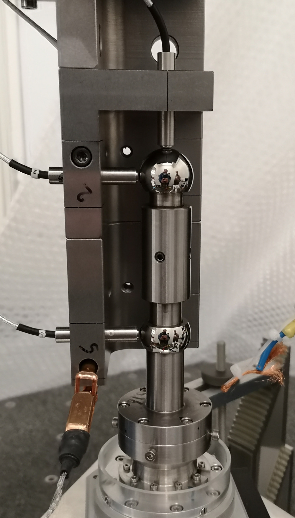
The two reference spheres are aligned with the rotation axis of the spindle. To do so, two measuring probes are used as shown in Figure ref:fig:test_id31_align_top_sphere_comparators.

To not damage the sensitive sphere surface, the probes are instead positioned on the cylinder on which the sphere is mounted. First, the probes are fixed to the bottom (fixed) cylinder to align the first sphere with the spindle axis. Then, the probes are fixed to the top (adjustable) cylinder, and the same alignment is performed.

With this setup, the alignment accuracy of both spheres with the spindle axis is expected to around $10\,\mu m$. The accuracy is probably limited due to the poor coaxiality between the cylinders and the spheres. However, this first alignment should permit to position the two sphere within the acceptance of the interferometers.

Tip-Tilt adjustment of the interferometers

<<ssec:test_id31_metrology_alignment>>

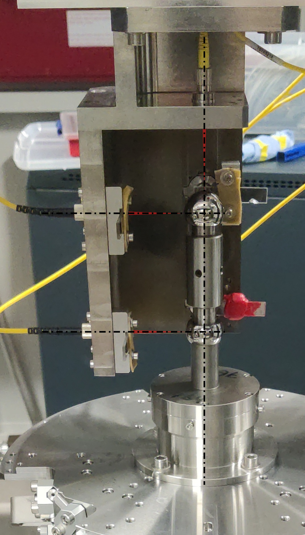
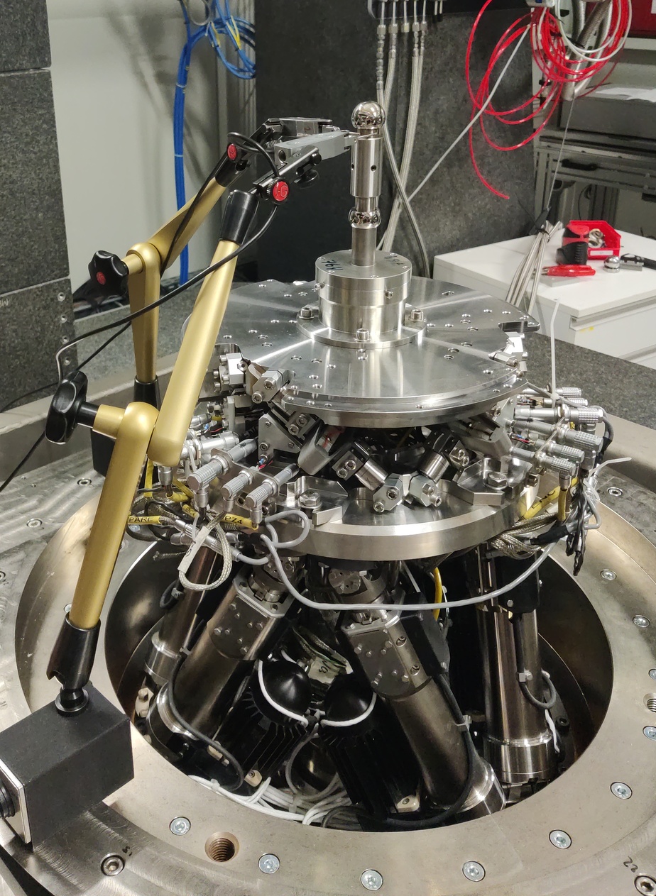
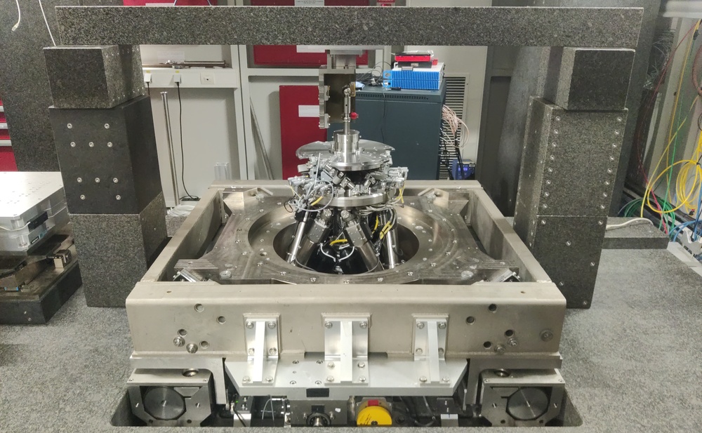
The short-stroke metrology system is placed on top of the main granite using a gantry made of granite blocs (Figure ref:fig:test_id31_short_stroke_metrology_overview). Granite is used to have good vibration and thermal stability.

The interferometer beams need to be position with respect to the two reference spheres as close as possible to the ideal case shown in Figure ref:fig:test_id31_metrology_kinematics. This means that their positions and angles needs to be well adjusted with respect to the two spheres. First, the vertical position of the spheres is adjusted using the micro-hexapod to match the height of the interferometers. Then, the horizontal position of the gantry is adjusted such that the coupling efficiency (i.e. the intensity of the light reflected back in the fiber) of the top interferometer is maximized. This is equivalent as to optimize the perpendicularity between the interferometer beam and the sphere surface (i.e. the concentricity between the top beam and the sphere center).

The lateral sensor heads (i.e. all except the top one) are each fixed to a custom tip-tilt adjustment mechanism. This allow to individually orient them such that they all point to the spheres' center (i.e. perpendicular to the sphere surface). This is done by maximizing the coupling efficiency of each interferometer.

After the alignment procedure, the top interferometer should coincide with with spindle axis, and the lateral interferometers should all be in the horizontal plane and intersect the spheres' center.

Fine Alignment of reference spheres using interferometers

<<ssec:test_id31_metrology_sphere_fine_alignment>>

Thanks to the first alignment of the two reference spheres with the spindle axis (Section ref:ssec:test_id31_metrology_sphere_rought_alignment) and to the fine adjustment of the interferometers orientations (Section ref:ssec:test_id31_metrology_alignment), the spindle can perform complete rotations while still having interference for all five interferometers. This metrology can therefore be used to better align the axis defined by the two spheres' center with the spindle axis.

The alignment process is made by few iterations. First, the spindle is scanned and the alignment errors are recorded. From the errors, the motion of the micro-hexapod to better align the spheres with the spindle axis is computed and the micro-hexapod is positioned accordingly. Then, the spindle is scanned again, and the new alignment errors are recorded.

This iterative process is first performed for angular errors (Figure ref:fig:test_id31_metrology_align_rx_ry) and then for lateral errors (Figure ref:fig:test_id31_metrology_align_dx_dy). The remaining errors after alignment is in the order of $\pm5\,\mu\text{rad}$ in $R_x$ and $R_y$ orientations, $\pm 1\,\mu m$ in $D_x$ and $D_y$ directions and less than $0.1\,\mu m$ vertically.

%% Angular alignment
% Load Data
data_it0 = h5scan(data_dir, 'alignment', 'h1rx_h1ry', 1);
data_it1 = h5scan(data_dir, 'alignment', 'h1rx_h1ry_0002', 3);
data_it2 = h5scan(data_dir, 'alignment', 'h1rx_h1ry_0002', 5);

% Offset wrong points
i_it0 = find(abs(data_it0.Rx_int_filtered(2:end)-data_it0.Rx_int_filtered(1:end-1))>1e-5);
data_it0.Rx_int_filtered(i_it0+1:end) = data_it0.Rx_int_filtered(i_it0+1:end) + data_it0.Rx_int_filtered(i_it0) - data_it0.Rx_int_filtered(i_it0+1);
i_it1 = find(abs(data_it1.Rx_int_filtered(2:end)-data_it1.Rx_int_filtered(1:end-1))>1e-5);
data_it1.Rx_int_filtered(i_it1+1:end) = data_it1.Rx_int_filtered(i_it1+1:end) + data_it1.Rx_int_filtered(i_it1) - data_it1.Rx_int_filtered(i_it1+1);
i_it2 = find(abs(data_it2.Rx_int_filtered(2:end)-data_it2.Rx_int_filtered(1:end-1))>1e-5);
data_it2.Rx_int_filtered(i_it2+1:end) = data_it2.Rx_int_filtered(i_it2+1:end) + data_it2.Rx_int_filtered(i_it2) - data_it2.Rx_int_filtered(i_it2+1);

% Compute circle fit and get radius
[~, ~, R_it0, ~] = circlefit(1e6*data_it0.Rx_int_filtered, 1e6*data_it0.Ry_int_filtered);
[~, ~, R_it1, ~] = circlefit(1e6*data_it1.Rx_int_filtered, 1e6*data_it1.Ry_int_filtered);
[~, ~, R_it2, ~] = circlefit(1e6*data_it2.Rx_int_filtered, 1e6*data_it2.Ry_int_filtered);

%% Eccentricity alignment
% Load Data
data_it0 = h5scan(data_dir, 'alignment', 'h1rx_h1ry_0002', 5);
data_it1 = h5scan(data_dir, 'alignment', 'h1dx_h1dy', 1);

% Offset wrong points
i_it0 = find(abs(data_it0.Dy_int_filtered(2:end)-data_it0.Dy_int_filtered(1:end-1))>1e-5);
data_it0.Dy_int_filtered(i_it0+1:end) = data_it0.Dy_int_filtered(i_it0+1:end) + data_it0.Dy_int_filtered(i_it0) - data_it0.Dy_int_filtered(i_it0+1);

% Compute circle fit and get radius
[~, ~, R_it0, ~] = circlefit(1e6*data_it0.Dx_int_filtered, 1e6*data_it0.Dy_int_filtered);
[~, ~, R_it1, ~] = circlefit(1e6*data_it1.Dx_int_filtered, 1e6*data_it1.Dy_int_filtered);

Estimated measurement volume

<<ssec:test_id31_metrology_acceptance>>

Because the interferometers are pointing to spheres and not flat surfaces, the lateral acceptance is limited. In order to estimate the metrology acceptance, the micro-hexapod is used to perform three accurate scans of $\pm 1\,mm$, respectively along the $x$, $y$ and $z$ axes. During these scans, the 5 interferometers are recorded individually, and the ranges in which each interferometer has enough coupling efficiency to be able to measure the displacement are estimated. Results are summarized in Table ref:tab:test_id31_metrology_acceptance. The obtained lateral acceptance for pure displacements in any direction is estimated to be around $+/-0.5\,mm$, which is enough for the current application as it is well above the micro-station errors to be actively corrected by the NASS.

%% Estimated acceptance of the metrology
% This is estimated by moving the spheres using the micro-hexapod

% Dx
data_dx = h5scan(data_dir, 'metrology_acceptance_new_align', 'dx', 1);

dx_acceptance = zeros(5,1);

for i = [1:size(dx_acceptance, 1)]
    % Find range in which the interferometers are measuring displacement
    dx_di = diff(data_dx.(sprintf('d%i', i))) == 0;
    if sum(dx_di) > 0
        dx_acceptance(i) = data_dx.h1tx(find(dx_di(501:end), 1) + 500) - ...
                           data_dx.h1tx(find(flip(dx_di(1:500)), 1));
    else
        dx_acceptance(i) = data_dx.h1tx(end) - data_dx.h1tx(1);
    end
end

% Dy
data_dy = h5scan(data_dir, 'metrology_acceptance_new_align', 'dy', 1);

dy_acceptance = zeros(5,1);

for i = [1:size(dy_acceptance, 1)]
    % Find range in which the interferometers are measuring displacement
    dy_di = diff(data_dy.(sprintf('d%i', i))) == 0;
    if sum(dy_di) > 0
        dy_acceptance(i) = data_dy.h1ty(find(dy_di(501:end), 1) + 500) - ...
                           data_dy.h1ty(find(flip(dy_di(1:500)), 1));
    else
        dy_acceptance(i) = data_dy.h1ty(end) - data_dy.h1ty(1);
    end
end

% Dz
data_dz = h5scan(data_dir, 'metrology_acceptance_new_align', 'dz', 1);

dz_acceptance = zeros(5,1);

for i = [1:size(dz_acceptance, 1)]
    % Find range in which the interferometers are measuring displacement
    dz_di = diff(data_dz.(sprintf('d%i', i))) == 0;
    if sum(dz_di) > 0
        dz_acceptance(i) = data_dz.h1tz(find(dz_di(501:end), 1) + 500) - ...
                           data_dz.h1tz(find(flip(dz_di(1:500)), 1));
    else
        dz_acceptance(i) = data_dz.h1tz(end) - data_dz.h1tz(1);
    end
end

	$D_x$	$D_y$	$D_z$
$d_1$ (y)	$1.0\,mm$	$>2\,mm$	$1.35\,mm$
$d_2$ (y)	$0.8\,mm$	$>2\,mm$	$1.01\,mm$
$d_3$ (x)	$>2\,mm$	$1.06\,mm$	$1.38\,mm$
$d_4$ (x)	$>2\,mm$	$0.99\,mm$	$0.94\,mm$
$d_5$ (z)	$1.33\, mm$	$1.06\,mm$	$>2\,mm$

Estimated measurement errors

<<ssec:test_id31_metrology_errors>>

When using the NASS, the accuracy of the sample's positioning is determined by the accuracy of the external metrology. However, the validation of the nano-hexapod, the associated instrumentation and the control architecture is independent of the accuracy of the metrology system. Only the bandwidth and noise characteristics of the external metrology are important. Yet, some elements effecting the accuracy of the metrology are discussed here.

First, the "metrology kinematics" (discussed in Section ref:ssec:test_id31_metrology_kinematics) is only approximate (i.e. valid for very small displacements). This can be easily seen when performing lateral $[D_x,\,D_y]$ scans using the micro-hexapod while recording the vertical interferometer (Figure ref:fig:test_id31_xy_map_sphere). As the interferometer is pointing to a sphere and not to a plane, lateral motion of the sphere is seen as a vertical motion by the top interferometer.

Then, the reference spheres have some deviations with respect to an ideal sphere ³. They are initially meant to be used with capacitive sensors which are integrating the shape errors over large surfaces. When using interferometers, the size of the "light spot" on the sphere surface is a circle with a diameter approximately equal to $50\,\mu m$, and therefore the measurement is more sensitive to shape errors with small features.

As the light from the interferometer is travelling through air (as opposed to being in vacuum), the measured distance is sensitive to any variation in the refractive index of the air. Therefore, any variation of air temperature, pressure or humidity will induce measurement errors. For instance, for a measurement length of $40\,mm$, a temperature variation of $0.1\,{}^oC$ (which is typical for the ID31 experimental hutch) induces an errors in the distance measurement of $\approx 4\,nm$.

Interferometers are also affected by noise cite:&watchi18_review_compac_inter. The effect of the noise on the translation and rotation measurements is estimated in Figure ref:fig:test_id31_interf_noise.

%% Interferometer noise estimation
data = load("test_id31_interf_noise.mat");

Ts = 1e-4;
Nfft = floor(5/Ts);
win = hanning(Nfft);
Noverlap = floor(Nfft/2);

[pxx_int, f] = pwelch(detrend(data.d, 0), win, Noverlap, Nfft, 1/Ts);

% Uncorrelated noise: square root of the sum of the squares
pxx_cart = pxx_int*sum(inv(Hm).^2, 2)';

rms_dxy = sqrt(trapz(f(f>1), pxx_cart((f>1),1))); % < 0.3 nm RMS
rms_dz  = sqrt(trapz(f(f>1), pxx_cart((f>1),3))); % < 0.3 nm RMS
rms_rxy = sqrt(trapz(f(f>1), pxx_cart((f>1),4))); % 5 nrad RMS

figure;
hold on;
plot(f, sqrt(pxx_cart(:,1)), 'DisplayName', sprintf('$D_{x,y}$, %.1f nmRMS', rms_dxy));
plot(f, sqrt(pxx_cart(:,3)), 'DisplayName', sprintf('$D_{z}$, %.1f nmRMS', rms_dz));
plot(f, sqrt(pxx_cart(:,4)), 'DisplayName', sprintf('$R_{x,y}$, %.1f nradRMS', rms_rxy));
set(gca, 'xscale', 'log'); set(gca, 'yscale', 'log');
xlabel('Frequency [Hz]'); ylabel('ASD $\left[\frac{nm,\ nrad}{\sqrt{Hz}}\right]$')
xlim([1, 1e3]); ylim([1e-3, 1]);
leg = legend('location', 'northeast', 'FontSize', 8, 'NumColumns', 1);
leg.ItemTokenSize(1) = 15;

%% X-Y scan with the micro-hexapod, and record of the vertical interferometer
data = h5scan(data_dir, 'metrology_acceptance', 'after_int_align_meshXY', 1);

x = 1e3*detrend(data.h1tx, 0); % [um]
y = 1e3*detrend(data.h1ty, 0); % [um]
z = 1e6*data.Dz_int_filtered - max(data.Dz_int_filtered); % [um]

mdl = scatteredInterpolant(x, y, z);
[xg, yg] = meshgrid(unique(x), unique(y));
zg = mdl(xg, yg);

% Fit a sphere to the data
[sphere_center,sphere_radius] = sphereFit(1e-3*[x, y, z]);

Open Loop Plant

<<sec:test_id31_open_loop_plant>>

Introduction   ignore

The NASS plant is schematically shown in Figure ref:fig:test_id31_block_schematic_plant. The input $\bm{u} = [u_1,\ u_2,\ u_3,\ u_4,\ u_5,\ u_6]$ is the command signal and corresponds to the voltages generated for each piezoelectric actuator. After amplification, the voltages across the piezoelectric stack actuators are $\bm{V}_a = [V_{a1},\ V_{a2},\ V_{a3},\ V_{a4},\ V_{a5},\ V_{a6}]$.

From the setpoint of micro-station stages ($r_{D_y}$ for the translation stage, $r_{R_y}$ for the tilt stage and $r_{R_z}$ for the spindle), the reference pose of the sample $\bm{r}_{\mathcal{X}}$ is computed using the micro-station's kinematics. The sample's position $\bm{y}_\mathcal{X} = [D_x,\,D_y,\,D_z,\,R_x,\,R_y,\,R_z]$ is measured using multiple sensors. First, the five interferometers $\bm{d} = [d_{1},\ d_{2},\ d_{3},\ d_{4},\ d_{5}]$ are used to measure the $[D_x,\,D_y,\,D_z,\,R_x,\,R_y]$ degrees of freedom of the sample. The $R_z$ position of the sample is computed from the spindle's setpoint $r_{R_z}$ and from the 6 encoders $\bm{d}_e$ integrated in the nano-hexapod.

The sample's position $\bm{y}_{\mathcal{X}}$ is compared to the reference position $\bm{r}_{\mathcal{X}}$ to compute the position error in the frame of the (rotating) nano-hexapod $\bm{\epsilon\mathcal{X}} = [\epsilon_{D_x},\,\epsilon_{D_y},\,\epsilon_{D_z},\,\epsilon_{R_x},\,\epsilon_{R_y},\,\epsilon_{R_z}]$. Finally, the Jacobian matrix $\bm{J}$ of the nano-hexapod is used to map $\bm{\epsilon\mathcal{X}}$ in the frame of the nano-hexapod struts $\bm{\epsilon\mathcal{L}} = [\epsilon_{\mathcal{L}_1},\,\epsilon_{\mathcal{L}_2},\,\epsilon_{\mathcal{L}_3},\,\epsilon_{\mathcal{L}_4},\,\epsilon_{\mathcal{L}_5},\,\epsilon_{\mathcal{L}_6}]$.

Voltages generated by the force sensor piezoelectric stacks $\bm{V}_s = [V_{s1},\ V_{s2},\ V_{s3},\ V_{s4},\ V_{s5},\ V_{s6}]$ will be used for active damping.

\begin{tikzpicture}
  % Blocs
  \node[block={2.0cm}{1.0cm}] (metrology) {Metrology};
  \node[block={2.0cm}{2.0cm}, below=0.1 of metrology, align=center] (nhexa) {Nano\\Hexapod};
  \node[block={4.0cm}{1.5cm}, below=0.1 of nhexa, align=center] (ustation) {Micro\\Station};

  \coordinate[] (inputVa)  at ($(nhexa.south west)!0.5!(nhexa.north west)$);
  \coordinate[] (outputVs) at ($(nhexa.south east)!0.3!(nhexa.north east)$);
  \coordinate[] (outputde) at ($(nhexa.south east)!0.7!(nhexa.north east)$);

  \coordinate[] (outputDy) at ($(ustation.south east)!0.1!(ustation.north east)$);
  \coordinate[] (outputRy) at ($(ustation.south east)!0.5!(ustation.north east)$);
  \coordinate[] (outputRz) at ($(ustation.south east)!0.9!(ustation.north east)$);

  \node[block={1.0cm}{1.0cm}, left=0.8 of inputVa] (pd200) {PD200};
  \node[block={1.0cm}{1.0cm}, right=0.8 of outputde] (Rz_kinematics) {$\bm{J}_{R_z}^{-1}$};
  \node[block={2.0cm}{2.0cm}, right=2.2 of ustation, align=center] (ustation_kinematics) {Compute\\Reference\\Position};
  \node[block={2.0cm}{2.0cm}, right=0.8 of ustation_kinematics, align=center] (compute_error) {Compute\\Error\\Position};
  \node[block={2.0cm}{2.0cm}, above=0.8 of compute_error, align=center] (compute_pos) {Compute\\Sample\\Position};
  \node[block={1.0cm}{1.0cm}, right=0.8 of compute_error] (hexa_jacobian) {$\bm{J}$};
  \node[block={1.0cm}{1.0cm}, right=0.8 of metrology] (metrology_kinematics) {$\bm{J}_d^{-1}$};

  \coordinate[] (inputMetrology) at ($(compute_error.north east)!0.3!(compute_error.north west)$);
  \coordinate[] (inputRz) at ($(compute_error.north east)!0.7!(compute_error.north west)$);

  \node[addb={+}{}{}{}{}, right=0.4 of Rz_kinematics] (addRz) {};
  \draw[->] (Rz_kinematics.east) -- (addRz.west);
  \draw[->] (outputRz-|addRz)node[branch]{} -- (addRz.south);

  \draw[->] (outputDy) node[above right]{$r_{D_y}$} -- (outputDy-|ustation_kinematics.west);
  \draw[->] (outputRy) node[above right]{$r_{R_y}$} -- (outputRy-|ustation_kinematics.west);
  \draw[->] (outputRz) node[above right]{$r_{R_z}$} -- (outputRz-|ustation_kinematics.west);

  % \draw[->] (outputVs) -- ++(0.8, 0) node[above left]{$\bm{V}_s$};

  \draw[->] (metrology.east) -- (metrology_kinematics.west) node[above left]{$\bm{d}$};

  \draw[->] (metrology_kinematics.east)node[above right]{$[D_x,\,D_y,\,D_z,\,R_x,\,R_y]$} -- (compute_pos.west|-metrology_kinematics);
  \draw[->] (addRz.east)node[above right]{$R_z$} -- (compute_pos.west|-addRz);
  \draw[->] (compute_pos.south)node -- (compute_error.north)node[above right]{$\bm{y}_{\mathcal{X}}$};

  \draw[->] (outputde) -- (Rz_kinematics.west) node[above left]{$\bm{d}_{e}$};
  \draw[->] (ustation_kinematics.east) -- (compute_error.west) node[above left]{$\bm{r}_{\mathcal{X}}$};
  \draw[->] (compute_error.east) -- (hexa_jacobian.west) node[above left]{$\bm{\epsilon\mathcal{X}}$};
  \draw[->] (hexa_jacobian.east) -- ++(0.8, 0)coordinate(eL) node[above left]{$\bm{\epsilon\mathcal{L}}$};
  \draw[->] (pd200.east) -- (inputVa) node[above left]{$\bm{V}_a$};
  \draw[<-] (pd200.west) -- ++(-0.8, 0) node[above right]{$\bm{u}$};

  \draw[->] (outputVs) -- (outputVs-|eL) node[above left]{$\bm{V}_s$};

  \begin{scope}[on background layer]
    \node[fit={(metrology.north-|pd200.west) (hexa_jacobian.east|-compute_error.south)}, fill=black!20!white, draw, dashed, inner sep=4pt] (plant) {};
    \node[anchor={north west}] at (plant.north west){$\text{Plant}$};
  \end{scope}
\end{tikzpicture}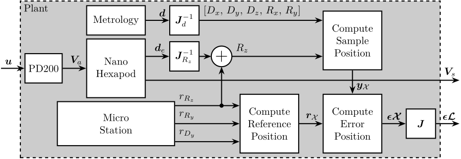

Schematic of the NASS plant

Open-Loop Plant Identification

<<ssec:test_id31_open_loop_plant_first_id>>

The plant dynamics is first identified for a fixed spindle angle (at $0\,\text{deg}$) and without any payload. The model dynamics is also identified in the same conditions.

A first comparison between the model and the measured dynamics is done in Figure ref:fig:test_id31_first_id. A good match can be observed for the diagonal dynamics (except the high frequency modes which are not modeled). However, the coupling for the transfer function from command signals $\bm{u}$ to the estimated strut motion from the external metrology $\bm{\epsilon\mathcal{L}}$ is larger than expected (Figure ref:fig:test_id31_first_id_int).

The experimental time delay estimated from the FRF (Figure ref:fig:test_id31_first_id_int) is larger than expected. After investigation, it was found that the additional delay was due to a digital processing unit⁴ that was used to get the interferometers' signals in the Speedgoat. This issue was later solved.

%% Identify the plant dynamics using the Simscape model

% Initialize each Simscape model elements
initializeGround();
initializeGranite();
initializeTy();
initializeRy();
initializeRz();
initializeMicroHexapod();
initializeNanoHexapod('flex_bot_type', '2dof', ...
                      'flex_top_type', '3dof', ...
                      'motion_sensor_type', 'plates', ...
                      'actuator_type', '2dof');
initializeSample('type', '0');

initializeSimscapeConfiguration('gravity', false);
initializeDisturbances('enable', false);
initializeLoggingConfiguration('log', 'none');
initializeController('type', 'open-loop');
initializeReferences();

% Input/Output definition
clear io; io_i = 1;
io(io_i) = linio([mdl, '/Controller'],     1, 'openinput');             io_i = io_i + 1; % Actuator Inputs [V]
io(io_i) = linio([mdl, '/Micro-Station'],  3, 'openoutput', [], 'Vs');  io_i = io_i + 1; % Force Sensors voltages [V]
io(io_i) = linio([mdl, '/Tracking Error'], 1, 'openoutput', [], 'EdL'); io_i = io_i + 1; % Position Errors [m]

% With no payload
Gm = exp(-1e-4*s)*linearize(mdl, io);
Gm.InputName  = {'u1', 'u2', 'u3', 'u4', 'u5', 'u6'};
Gm.OutputName = {'Vs1', 'Vs2', 'Vs3', 'Vs4', 'Vs5', 'Vs6', ...
                 'eL1', 'eL2', 'eL3', 'eL4', 'eL5', 'eL6'};

%% Identify the plant from experimental data

% Load identification data
data = load('2023-08-08_16-17_ol_plant_m0_Wz0.mat');

% Frequency analysis parameters
Ts = 1e-4; % Sampling Time [s]
Nfft = floor(2.0/Ts);
win = hanning(Nfft);
Noverlap = floor(Nfft/2);
[~, f] = tfestimate(data.uL1.id_plant, data.uL1.e_L1, win, Noverlap, Nfft, 1/Ts);

G_iff = zeros(length(f), 6, 6); % Force sensor outputs
G_int = zeros(length(f), 6, 6); % Estimated strut errors
for i_strut = 1:6
    Vs = [data.(sprintf("uL%i", i_strut)).Vs1 ; data.(sprintf("uL%i", i_strut)).Vs2 ; data.(sprintf("uL%i", i_strut)).Vs3 ; data.(sprintf("uL%i", i_strut)).Vs4 ; data.(sprintf("uL%i", i_strut)).Vs5 ; data.(sprintf("uL%i", i_strut)).Vs6]';
    eL = [data.(sprintf("uL%i", i_strut)).e_L1 ; data.(sprintf("uL%i", i_strut)).e_L2 ; data.(sprintf("uL%i", i_strut)).e_L3 ; data.(sprintf("uL%i", i_strut)).e_L4 ; data.(sprintf("uL%i", i_strut)).e_L5 ; data.(sprintf("uL%i", i_strut)).e_L6]';
    dL = [data.(sprintf("uL%i", i_strut)).dL1 ; data.(sprintf("uL%i", i_strut)).dL2 ; data.(sprintf("uL%i", i_strut)).dL3 ; data.(sprintf("uL%i", i_strut)).dL4 ; data.(sprintf("uL%i", i_strut)).dL5 ; data.(sprintf("uL%i", i_strut)).dL6]';

    G_iff(:,:,i_strut) = tfestimate(data.(sprintf("uL%i", i_strut)).id_plant, Vs, win, Noverlap, Nfft, 1/Ts);
    G_int(:,:,i_strut) = tfestimate(data.(sprintf("uL%i", i_strut)).id_plant, eL, win, Noverlap, Nfft, 1/Ts);
end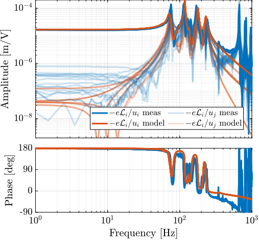

Better Angular Alignment

<<ssec:test_id31_open_loop_plant_rz_alignment>>

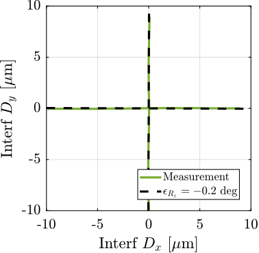
One possible explanation of the increased coupling observed in Figure ref:fig:test_id31_first_id_int is the poor alignment between the external metrology axes (i.e. the interferometer supports) and the nano-hexapod axes. To estimate this alignment, a decentralized low-bandwidth feedback controller based on the nano-hexapod encoders was implemented. This allowed to perform two straight movements of the nano-hexapod along its $x$ and $y$ axes. During these two movements, the external metrology measurement was recorded and are shown in Figure ref:fig:test_id31_Rz_align_error. It was found that there is a misalignment of 2.7 degrees (rotation along the vertical axis) between the interferometer axes and nano-hexapod axes. This was corrected by adding an offset to the spindle angle. After alignment, the same movement was performed using the nano-hexapod while recording the signal of the external metrology. Results shown in Figure ref:fig:test_id31_Rz_align_correct are indeed indicating much better alignment.

%% Load Data
data_1_dx = h5scan(data_dir, 'align_int_enc_Rz', 'tx_first_scan', 2);
data_1_dy = h5scan(data_dir, 'align_int_enc_Rz', 'tx_first_scan', 3);
data_2_dx = h5scan(data_dir, 'align_int_enc_Rz', 'verif-after-correct-offset', 1);
data_2_dy = h5scan(data_dir, 'align_int_enc_Rz', 'verif-after-correct-offset', 2);

% Estimation of Rz misalignment
p1 = polyfit(data_1_dx.Dx_int_filtered, data_1_dx.Dy_int_filtered, 1);
p2 = polyfit(data_1_dy.Dx_int_filtered, data_1_dy.Dy_int_filtered, 1);

Rz_error = (atan(p1(1)) + atan(p2(1))-pi/2)/2; % ~3 degrees

%% Estimation of the Rz misalignment
figure;
hold on;
plot(1e6*data_1_dx.Dx_int_filtered, 1e6*data_1_dx.Dy_int_filtered, 'color', colors(2,:), 'DisplayName', 'Measurement')
plot(1e6*data_1_dy.Dx_int_filtered, 1e6*data_1_dy.Dy_int_filtered, 'color', colors(2,:), 'HandleVisibility', 'off')
plot( 1e6*[-10:10]*cos(Rz_error), 1e6*[-10:10]*sin(Rz_error), 'k--', 'DisplayName', sprintf('$\\epsilon_{R_z} = %.1f$ deg', Rz_error*180/pi))
plot(-1e6*[-10:10]*sin(Rz_error), 1e6*[-10:10]*cos(Rz_error), 'k--', 'HandleVisibility', 'off')
hold off;
xlabel('Interf $D_x$ [$\mu$m]');
ylabel('Interf $D_y$ [$\mu$m]');
axis equal
xlim([-10, 10]); ylim([-10, 10]);
xticks([-10:5:10]); yticks([-10:5:10]);
leg = legend('location', 'southeast', 'FontSize', 8, 'NumColumns', 1);
leg.ItemTokenSize(1) = 15;

% Estimation of Rz misalignment after correcting the Rz angle
p1 = polyfit(data_2_dx.Dx_int_filtered, data_2_dx.Dy_int_filtered, 1);
p2 = polyfit(data_2_dy.Dx_int_filtered, data_2_dy.Dy_int_filtered, 1);

Rz_error = (atan(p1(1)) + atan(p2(1))-pi/2)/2; % ~0.2 degrees

%% Estimation of the Rz misalignment after correcting the Rz offset
figure;
hold on;
plot(1e6*data_2_dx.Dx_int_filtered, 1e6*data_2_dx.Dy_int_filtered, 'color', colors(5,:), 'DisplayName', 'Measurement')
plot(1e6*data_2_dy.Dx_int_filtered, 1e6*data_2_dy.Dy_int_filtered, 'color', colors(5,:), 'HandleVisibility', 'off')
plot( 1e6*[-10:10]*cos(Rz_error), 1e6*[-10:10]*sin(Rz_error), 'k--', 'DisplayName', sprintf('$\\epsilon_{R_z} = %.1f$ deg', Rz_error*180/pi))
plot(-1e6*[-10:10]*sin(Rz_error), 1e6*[-10:10]*cos(Rz_error), 'k--', 'HandleVisibility', 'off')
hold off;
xlabel('Interf $D_x$ [$\mu$m]');
ylabel('Interf $D_y$ [$\mu$m]');
axis equal
xlim([-10, 10]); ylim([-10, 10]);
xticks([-10:5:10]); yticks([-10:5:10]);
leg = legend('location', 'southeast', 'FontSize', 8, 'NumColumns', 1);
leg.ItemTokenSize(1) = 15;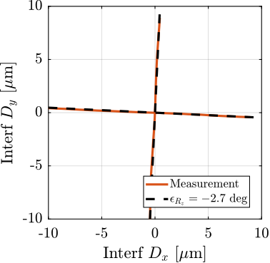

The plant dynamics was identified again after the fine alignment and is compared with the model dynamics in Figure ref:fig:test_id31_first_id_int_better_rz_align. Compared to the initial identification shown in Figure ref:fig:test_id31_first_id_int, the obtained coupling has decreased and is now close to the coupling obtained with the multi-body model. At low frequency (below $10\,\text{Hz}$) all the off-diagonal elements have an amplitude $\approx 100$ times lower compared to the diagonal elements, indicating that a low bandwidth feedback controller can be implemented in a decentralized way (i.e. $6$ SISO controllers). Between $650\,\text{Hz}$ and $1000\,\text{Hz}$, several modes can be observed that are due to flexible modes of the top platform and modes of the two spheres adjustment mechanism. The flexible modes of the top platform can be passively damped while the modes of the two reference spheres should not be present in the final application.

%% Identification of the plant after Rz alignment
data_align = load('2023-08-17_17-37_ol_plant_m0_Wz0_new_Rz_align.mat');

G_int_align = zeros(length(f), 6, 6);
for i_strut = 1:6
    eL = [data_align.(sprintf("uL%i", i_strut)).e_L1 ; data_align.(sprintf("uL%i", i_strut)).e_L2 ; data_align.(sprintf("uL%i", i_strut)).e_L3 ; data_align.(sprintf("uL%i", i_strut)).e_L4 ; data_align.(sprintf("uL%i", i_strut)).e_L5 ; data_align.(sprintf("uL%i", i_strut)).e_L6]';

    G_int_align(:,:,i_strut) = tfestimate(data_align.(sprintf("uL%i", i_strut)).id_plant, eL, win, Noverlap, Nfft, 1/Ts);
end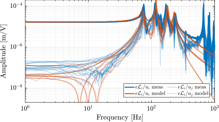

Decrease of the coupling with better Rz alignment

Effect of Payload Mass

<<ssec:test_id31_open_loop_plant_mass>>

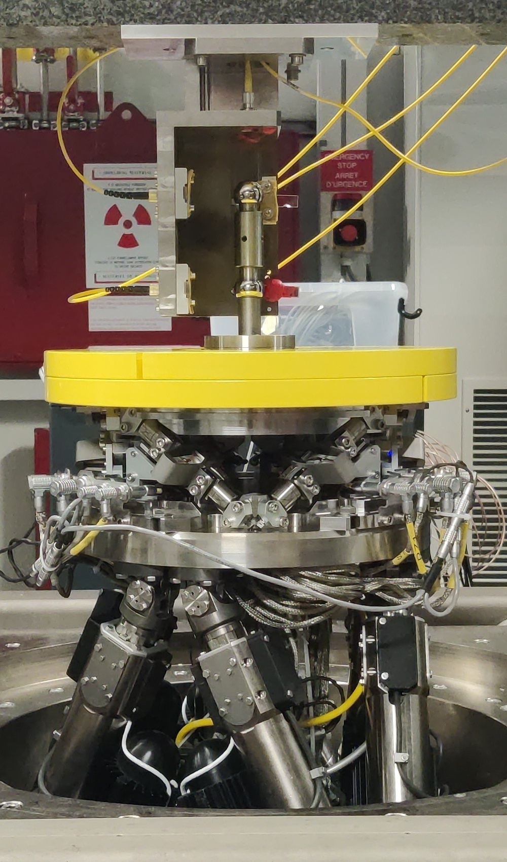
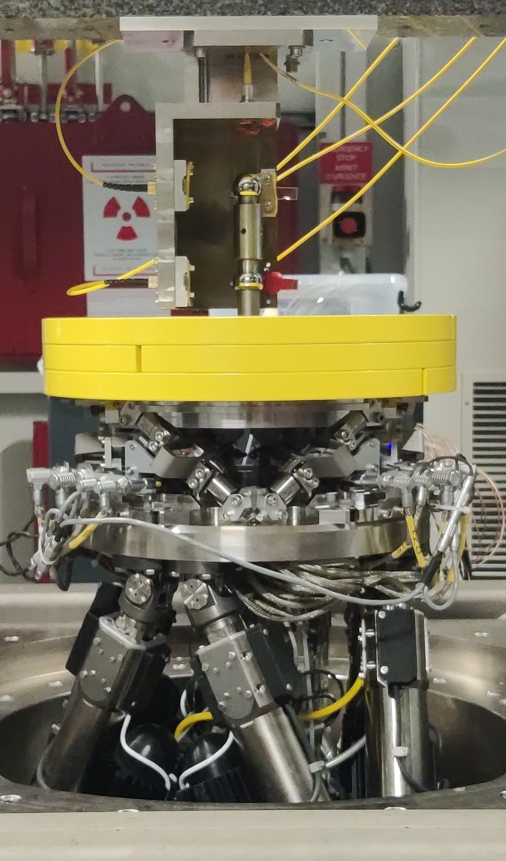
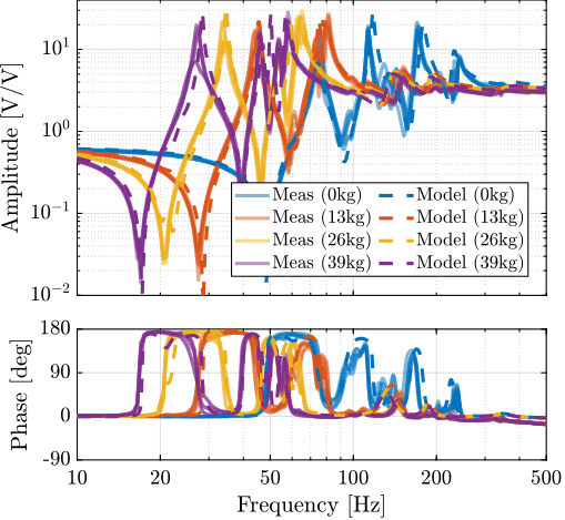
In order to see how the system dynamics changes with the payload, open-loop identification was performed for four payload conditions that are shown in Figure ref:fig:test_id31_picture_masses. The obtained direct terms are compared with the model dynamics in Figure ref:fig:test_id31_comp_simscape_diag_masses. It is shown that the model dynamics well predicts the measured dynamics for all payload conditions. Therefore the model can be used for model-based control is necessary.

It is interesting to note that the anti-resonances in the force sensor plant are now appearing as minimum-phase, as the model predicts (Figure ref:fig:test_id31_comp_simscape_iff_diag_masses).

%% Identify the plant from experimental data - All payloads

% Load identification data
data_m0_Wz0 = load('2023-08-08_16-17_ol_plant_m0_Wz0.mat');
data_m1_Wz0 = load('2023-08-08_18-57_ol_plant_m1_Wz0.mat');
data_m2_Wz0 = load('2023-08-08_17-12_ol_plant_m2_Wz0.mat');
data_m3_Wz0 = load('2023-08-08_18-20_ol_plant_m3_Wz0.mat');

% Sampling Time [s]
Ts = 1e-4;

% Hannning Windows
Nfft = floor(2.0/Ts);
win = hanning(Nfft);
Noverlap = floor(Nfft/2);

% And we get the frequency vector
[~, f] = tfestimate(data_m0_Wz0.uL1.id_plant, data_m0_Wz0.uL1.e_L1, win, Noverlap, Nfft, 1/Ts);

% No payload
G_iff_m0_Wz0 = zeros(length(f), 6, 6);
for i_strut = 1:6
    eL = [data_m0_Wz0.(sprintf("uL%i", i_strut)).Vs1 ; data_m0_Wz0.(sprintf("uL%i", i_strut)).Vs2 ; data_m0_Wz0.(sprintf("uL%i", i_strut)).Vs3 ; data_m0_Wz0.(sprintf("uL%i", i_strut)).Vs4 ; data_m0_Wz0.(sprintf("uL%i", i_strut)).Vs5 ; data_m0_Wz0.(sprintf("uL%i", i_strut)).Vs6]';

    G_iff_m0_Wz0(:,:,i_strut) = tfestimate(data_m0_Wz0.(sprintf("uL%i", i_strut)).id_plant, eL, win, Noverlap, Nfft, 1/Ts);
end

G_int_m0_Wz0 = zeros(length(f), 6, 6);
for i_strut = 1:6
    eL = [data_m0_Wz0.(sprintf("uL%i", i_strut)).e_L1 ; data_m0_Wz0.(sprintf("uL%i", i_strut)).e_L2 ; data_m0_Wz0.(sprintf("uL%i", i_strut)).e_L3 ; data_m0_Wz0.(sprintf("uL%i", i_strut)).e_L4 ; data_m0_Wz0.(sprintf("uL%i", i_strut)).e_L5 ; data_m0_Wz0.(sprintf("uL%i", i_strut)).e_L6]';

    G_int_m0_Wz0(:,:,i_strut) = tfestimate(data_m0_Wz0.(sprintf("uL%i", i_strut)).id_plant, eL, win, Noverlap, Nfft, 1/Ts);
end

% 1 "payload layer"
G_iff_m1_Wz0 = zeros(length(f), 6, 6);
for i_strut = 1:6
    eL = [data_m1_Wz0.(sprintf("uL%i", i_strut)).Vs1 ; data_m1_Wz0.(sprintf("uL%i", i_strut)).Vs2 ; data_m1_Wz0.(sprintf("uL%i", i_strut)).Vs3 ; data_m1_Wz0.(sprintf("uL%i", i_strut)).Vs4 ; data_m1_Wz0.(sprintf("uL%i", i_strut)).Vs5 ; data_m1_Wz0.(sprintf("uL%i", i_strut)).Vs6]';

    G_iff_m1_Wz0(:,:,i_strut) = tfestimate(data_m1_Wz0.(sprintf("uL%i", i_strut)).id_plant, eL, win, Noverlap, Nfft, 1/Ts);
end

G_int_m1_Wz0 = zeros(length(f), 6, 6);
for i_strut = 1:6
    eL = [data_m1_Wz0.(sprintf("uL%i", i_strut)).e_L1 ; data_m1_Wz0.(sprintf("uL%i", i_strut)).e_L2 ; data_m1_Wz0.(sprintf("uL%i", i_strut)).e_L3 ; data_m1_Wz0.(sprintf("uL%i", i_strut)).e_L4 ; data_m1_Wz0.(sprintf("uL%i", i_strut)).e_L5 ; data_m1_Wz0.(sprintf("uL%i", i_strut)).e_L6]';

    G_int_m1_Wz0(:,:,i_strut) = tfestimate(data_m1_Wz0.(sprintf("uL%i", i_strut)).id_plant, eL, win, Noverlap, Nfft, 1/Ts);
end

% 2 "payload layers"
G_iff_m2_Wz0 = zeros(length(f), 6, 6);
for i_strut = 1:6
    eL = [data_m2_Wz0.(sprintf("uL%i", i_strut)).Vs1 ; data_m2_Wz0.(sprintf("uL%i", i_strut)).Vs2 ; data_m2_Wz0.(sprintf("uL%i", i_strut)).Vs3 ; data_m2_Wz0.(sprintf("uL%i", i_strut)).Vs4 ; data_m2_Wz0.(sprintf("uL%i", i_strut)).Vs5 ; data_m2_Wz0.(sprintf("uL%i", i_strut)).Vs6]';

    G_iff_m2_Wz0(:,:,i_strut) = tfestimate(data_m2_Wz0.(sprintf("uL%i", i_strut)).id_plant, eL, win, Noverlap, Nfft, 1/Ts);
end

G_int_m2_Wz0 = zeros(length(f), 6, 6);
for i_strut = 1:6
    eL = [data_m2_Wz0.(sprintf("uL%i", i_strut)).e_L1 ; data_m2_Wz0.(sprintf("uL%i", i_strut)).e_L2 ; data_m2_Wz0.(sprintf("uL%i", i_strut)).e_L3 ; data_m2_Wz0.(sprintf("uL%i", i_strut)).e_L4 ; data_m2_Wz0.(sprintf("uL%i", i_strut)).e_L5 ; data_m2_Wz0.(sprintf("uL%i", i_strut)).e_L6]';

    G_int_m2_Wz0(:,:,i_strut) = tfestimate(data_m2_Wz0.(sprintf("uL%i", i_strut)).id_plant, eL, win, Noverlap, Nfft, 1/Ts);
end

% 3 "payload layers"
G_iff_m3_Wz0 = zeros(length(f), 6, 6);
for i_strut = 1:6
    eL = [data_m3_Wz0.(sprintf("uL%i", i_strut)).Vs1 ; data_m3_Wz0.(sprintf("uL%i", i_strut)).Vs2 ; data_m3_Wz0.(sprintf("uL%i", i_strut)).Vs3 ; data_m3_Wz0.(sprintf("uL%i", i_strut)).Vs4 ; data_m3_Wz0.(sprintf("uL%i", i_strut)).Vs5 ; data_m3_Wz0.(sprintf("uL%i", i_strut)).Vs6]';

    G_iff_m3_Wz0(:,:,i_strut) = tfestimate(data_m3_Wz0.(sprintf("uL%i", i_strut)).id_plant, eL, win, Noverlap, Nfft, 1/Ts);
end

G_int_m3_Wz0 = zeros(length(f), 6, 6);
for i_strut = 1:6
    eL = [data_m3_Wz0.(sprintf("uL%i", i_strut)).e_L1 ; data_m3_Wz0.(sprintf("uL%i", i_strut)).e_L2 ; data_m3_Wz0.(sprintf("uL%i", i_strut)).e_L3 ; data_m3_Wz0.(sprintf("uL%i", i_strut)).e_L4 ; data_m3_Wz0.(sprintf("uL%i", i_strut)).e_L5 ; data_m3_Wz0.(sprintf("uL%i", i_strut)).e_L6]';

    G_int_m3_Wz0(:,:,i_strut) = tfestimate(data_m3_Wz0.(sprintf("uL%i", i_strut)).id_plant, eL, win, Noverlap, Nfft, 1/Ts);
end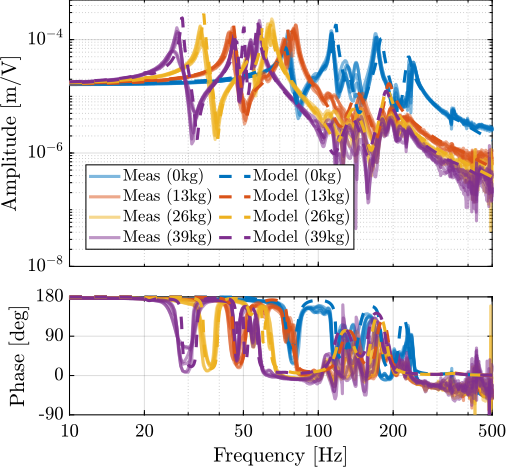

Effect of Spindle Rotation

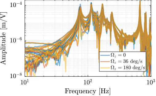
<<ssec:test_id31_open_loop_plant_rotation>>

To verify that all the kinematics in Figure ref:fig:test_id31_block_schematic_plant are correct and to check whether the system dynamics is affected by Spindle rotation of not, three identification experiments were performed: no spindle rotation, spindle rotation at $36\,\text{deg}/s$ and at $180\,\text{deg}/s$.

The comparison of the obtained dynamics from command signal $u$ to estimated strut error $\epsilon\mathcal{L}$ is done in Figure ref:fig:test_id31_effect_rotation. Both direct terms (Figure ref:fig:test_id31_effect_rotation_direct) and coupling terms (Figure ref:fig:test_id31_effect_rotation_coupling) are unaffected by the rotation. The same can be observed for the dynamics from the command signal to the encoders and to the force sensors. This confirms that the rotation has no significant effect on the plant dynamics. This also indicates that the metrology kinematics is correct and is working in real time.

%% Identify the model dynamics with Spindle rotation
initializeSample('type', '0');
initializeReferences(...
    'Rz_type', 'rotating', ...
    'Rz_period', 360/36); % 36 deg/s, 6rpm
Gm_m0_Wz36 = linearize(mdl, io, 0.1);
Gm_m0_Wz36.InputName  = {'u1', 'u2', 'u3', 'u4', 'u5', 'u6'};
Gm_m0_Wz36.OutputName = {'Vs1', 'Vs2', 'Vs3', 'Vs4', 'Vs5', 'Vs6', ...
                         'eL1', 'eL2', 'eL3', 'eL4', 'eL5', 'eL6'};

initializeReferences(...
    'Rz_type', 'rotating', ...
    'Rz_period', 360/180); % 180 deg/s, 30rpm
Gm_m0_Wz180 = linearize(mdl, io, 0.1);
Gm_m0_Wz180.InputName  = {'u1', 'u2', 'u3', 'u4', 'u5', 'u6'};
Gm_m0_Wz180.OutputName = {'Vs1', 'Vs2', 'Vs3', 'Vs4', 'Vs5', 'Vs6', ...
                          'eL1', 'eL2', 'eL3', 'eL4', 'eL5', 'eL6'};

%% Identify the plant from experimental data - Effect of rotation

% Load identification data
data_m0_Wz36  = load('2023-08-08_16-28_ol_plant_m0_Wz36.mat');
data_m0_Wz180 = load('2023-08-08_16-45_ol_plant_m0_Wz180.mat');

% Spindle Rotation at 36 deg/s
G_iff_m0_Wz36 = zeros(length(f), 6, 6);
for i_strut = 1:6
    eL = [data_m0_Wz36.(sprintf("uL%i", i_strut)).Vs1 ; data_m0_Wz36.(sprintf("uL%i", i_strut)).Vs2 ; data_m0_Wz36.(sprintf("uL%i", i_strut)).Vs3 ; data_m0_Wz36.(sprintf("uL%i", i_strut)).Vs4 ; data_m0_Wz36.(sprintf("uL%i", i_strut)).Vs5 ; data_m0_Wz36.(sprintf("uL%i", i_strut)).Vs6]';

    G_iff_m0_Wz36(:,:,i_strut) = tfestimate(data_m0_Wz36.(sprintf("uL%i", i_strut)).id_plant, eL, win, Noverlap, Nfft, 1/Ts);
end

G_int_m0_Wz36 = zeros(length(f), 6, 6);
for i_strut = 1:6
    eL = [data_m0_Wz36.(sprintf("uL%i", i_strut)).e_L1 ; data_m0_Wz36.(sprintf("uL%i", i_strut)).e_L2 ; data_m0_Wz36.(sprintf("uL%i", i_strut)).e_L3 ; data_m0_Wz36.(sprintf("uL%i", i_strut)).e_L4 ; data_m0_Wz36.(sprintf("uL%i", i_strut)).e_L5 ; data_m0_Wz36.(sprintf("uL%i", i_strut)).e_L6]';

    G_int_m0_Wz36(:,:,i_strut) = tfestimate(data_m0_Wz36.(sprintf("uL%i", i_strut)).id_plant, eL, win, Noverlap, Nfft, 1/Ts);
end

% Spindle Rotation at 180 deg/s
G_iff_m0_Wz180 = zeros(length(f), 6, 6);
for i_strut = 1:6
    eL = [data_m0_Wz180.(sprintf("uL%i", i_strut)).Vs1 ; data_m0_Wz180.(sprintf("uL%i", i_strut)).Vs2 ; data_m0_Wz180.(sprintf("uL%i", i_strut)).Vs3 ; data_m0_Wz180.(sprintf("uL%i", i_strut)).Vs4 ; data_m0_Wz180.(sprintf("uL%i", i_strut)).Vs5 ; data_m0_Wz180.(sprintf("uL%i", i_strut)).Vs6]';

    G_iff_m0_Wz180(:,:,i_strut) = tfestimate(data_m0_Wz180.(sprintf("uL%i", i_strut)).id_plant, eL, win, Noverlap, Nfft, 1/Ts);
end

G_int_m0_Wz180 = zeros(length(f), 6, 6);
for i_strut = 1:6
    eL = [data_m0_Wz180.(sprintf("uL%i", i_strut)).e_L1 ; data_m0_Wz180.(sprintf("uL%i", i_strut)).e_L2 ; data_m0_Wz180.(sprintf("uL%i", i_strut)).e_L3 ; data_m0_Wz180.(sprintf("uL%i", i_strut)).e_L4 ; data_m0_Wz180.(sprintf("uL%i", i_strut)).e_L5 ; data_m0_Wz180.(sprintf("uL%i", i_strut)).e_L6]';

    G_int_m0_Wz180(:,:,i_strut) = tfestimate(data_m0_Wz180.(sprintf("uL%i", i_strut)).id_plant, eL, win, Noverlap, Nfft, 1/Ts);
end

% The identified dynamics are then saved for further use.
save('./mat/test_id31_simscape_open_loop_plants.mat', 'Gm_m0_Wz0', 'Gm_m0_Wz36', 'Gm_m0_Wz180', 'Gm_m1_Wz0', 'Gm_m2_Wz0', 'Gm_m3_Wz0');
save('./mat/test_id31_identified_open_loop_plants.mat', 'G_int_m0_Wz0', 'G_int_m0_Wz36', 'G_int_m0_Wz180', 'G_int_m1_Wz0', 'G_int_m2_Wz0', 'G_int_m3_Wz0', ...
                                                        'G_iff_m0_Wz0', 'G_iff_m0_Wz36', 'G_iff_m0_Wz180', 'G_iff_m1_Wz0', 'G_iff_m2_Wz0', 'G_iff_m3_Wz0', 'f');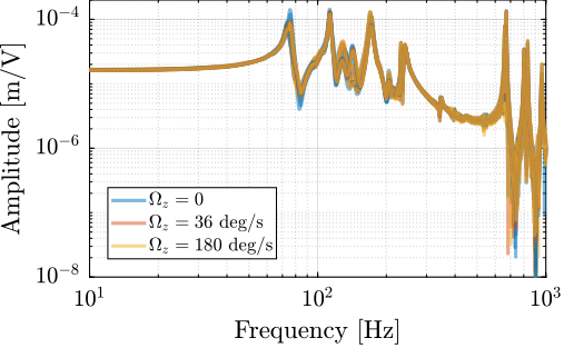

Conclusion

The identified frequency response functions from command signals $\bm{u}$ to the force sensors $\bm{V}_s$ and to the estimated strut errors $\bm{\epsilon\mathcal{L}}$ are well matching the developed multi-body model. Effect of payload mass is shown to be well predicted by the model, which can be useful if robust model based control is to be used. The spindle rotation has no visible effect on the measured dynamics, indicating that controllers should be robust to the spindle rotation.

Decentralized Integral Force Feedback

<<sec:test_id31_iff>>

Introduction   ignore

The HAC-LAC strategy that was previously developed and validated using the multi-body model is now experimentally implemented.

In this section, the low authority control part is first validated. It consisted of a decentralized Integral Force Feedback controller $\bm{K}_{\text{IFF}}$, with all the diagonal terms being equal eqref:eq:test_id31_Kiff.

\begin{equation}\label{eq:test_id31_iff_diagonal} \bm{K}_{\text{IFF}} = K_{\text{IFF}} ⋅ \bm{I}_6 = \begin{bmatrix} K_{\text{IFF}} & & 0
& \ddots &
0 & & K_{\text{IFF}}

\end{bmatrix}

\end{equation}

And it is implemented as shown in the block diagram of Figure ref:fig:test_id31_iff_block_diagram.

\begin{tikzpicture}
  % Blocs
  \node[block={2.0cm}{2.0cm}] (P) {Plant};
  \coordinate[] (input)   at ($(P.south west)!0.5!(P.north west)$);
  \coordinate[] (outputH) at ($(P.south east)!0.2!(P.north east)$);
  \coordinate[] (outputL) at ($(P.south east)!0.8!(P.north east)$);

  \node[block, above=0.6 of P] (Klac) {$\bm{K}_\text{IFF}$};
  \node[addb, left= of input] (addF) {};

  % Connections and labels
  \draw[->] (outputL) -- ++(0.6, 0) coordinate(eastlac) |- (Klac.east);
  \node[above right] at (outputL){$\bm{V}_s$};
  \draw[->] (Klac.west) -| (addF.north);
  \draw[->] (addF.east) -- (input) node[above left]{$\bm{u}$};

  \draw[->] (outputH) -- ++(1.6, 0) node[above left]{$\bm{\epsilon\mathcal{L}}$};
  \draw[<-] (addF.west) -- ++(-1.0, 0) node[above right]{$\bm{u^{\prime}}$};

  \begin{scope}[on background layer]
    \node[fit={(Klac.north-|eastlac) (addF.west|-P.south)}, fill=black!20!white, draw, dashed, inner sep=10pt] (Pi) {};
    \node[anchor={north west}] at (Pi.north west){$\text{Damped Plant}$};
  \end{scope}
\end{tikzpicture}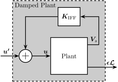

Block diagram of the implemented decentralized IFF controller. The controller $\bm{K}_{\text{IFF}}$ is a diagonal controller with the same elements on every diagonal term $K_{\text{IFF}}$.

IFF Plant

<<ssec:test_id31_iff_plant>>

As the multi-body model is going to be used to evaluate the stability of the IFF controller and to optimize the achievable damping, it is first checked whether this model accurately represents the system dynamics.

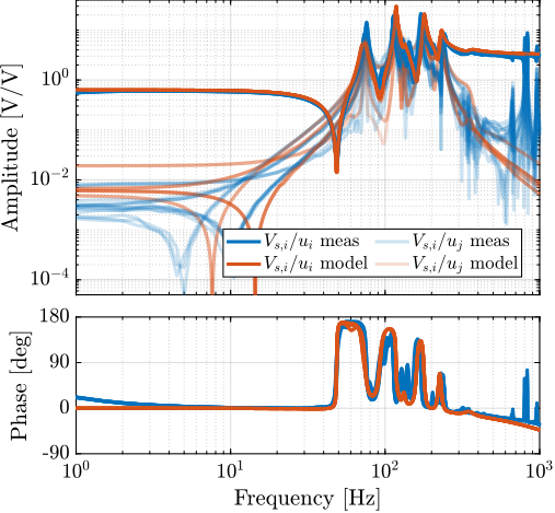
In the previous section (Figure ref:fig:test_id31_comp_simscape_iff_diag_masses), it was shown that the model well captures the dynamics from each actuator to its collocated force sensor, and that for all considered payloads. Nevertheless, it is also important to well model the coupling in the system. To very that, instead of comparing the 36 elements of the $6 \times 6$ frequency response matrix from $\bm{u}$ to $\bm{V_s}$, only 6 elements are compared in Figure ref:fig:test_id31_comp_simscape_Vs. Similar results are obtained for all other 30 elements and for the different tested payload conditions. This confirms that the multi-body model can be used to tune the IFF controller.

% Load identified FRF for IFF Plant and Multi-Body Model
load('test_id31_identified_open_loop_plants.mat', 'G_iff_m0_Wz0', 'G_iff_m1_Wz0', 'G_iff_m2_Wz0', 'G_iff_m3_Wz0', 'f');
load('test_id31_simscape_open_loop_plants.mat', 'Gm_m0_Wz0', 'Gm_m1_Wz0', 'Gm_m2_Wz0', 'Gm_m3_Wz0');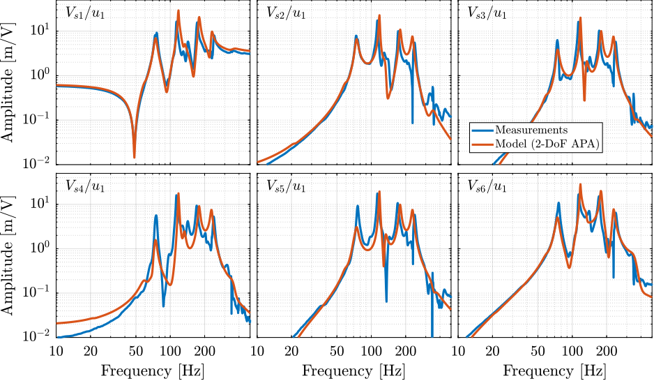

Comparison of the measured (in blue) and modeled (in red) frequency transfer functions from the first control signal $u_1$ to the six force sensor voltages $V_{s1}$ to $V_{s6}$

IFF Controller

<<ssec:test_id31_iff_controller>>

A decentralized IFF controller was designed such that it adds damping to the suspension modes of the nano-hexapod for all considered payloads. The frequency of the suspension modes are ranging from $\approx 30\,\text{Hz}$ to $\approx 250\,\text{Hz}$ (Figure ref:fig:test_id31_comp_simscape_iff_diag_masses), and therefore the IFF controller should provide integral action in this frequency range. A second order high pass filter (cut-off frequency of $10\,\text{Hz}$) was added to limit the low frequency gain eqref:eq:test_id31_Kiff.

\begin{equation}\label{eq:test_id31_Kiff} K_{\text{IFF}} = g_0 ⋅ _brace{\frac{1}{s}}_{\text{int}} ⋅ _brace{\frac{s^2/ω_z^2}{s^2/ω_z^2 + 2ξ_z s /ω_z + 1}}_{\text{2nd order LPF}},\quad ≤ft(g_0 = -100,\ ω_z = 2π10\,\text{rad/s},\ ξ_z = 0.7\right)

\end{equation}

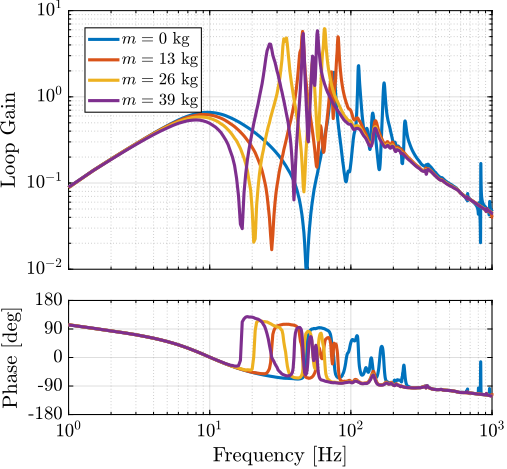
The bode plot of the decentralized IFF controller is shown in Figure ref:fig:test_id31_Kiff_bode_plot and the "decentralized loop-gains" for all considered payload masses are shown in Figure ref:fig:test_id31_Kiff_loop_gain. It can be seen that the loop-gain is larger than $1$ around suspension modes indicating that some damping should be added to the suspension modes.

%% IFF Controller Design
% Second order high pass filter
wz = 2*pi*10;
xiz = 0.7;
Ghpf = (s^2/wz^2)/(s^2/wz^2 + 2*xiz*s/wz + 1);

% IFF Controller
Kiff = -1e2 * ...              % Gain
       1/(0.01*2*pi + s) * ... % LPF: provides integral action
       Ghpf * ...              % 2nd order HPF (limit low frequency gain)
       eye(6);                 % Diagonal 6x6 controller (i.e. decentralized)

Kiff.InputName = {'Vs1', 'Vs2', 'Vs3', 'Vs4', 'Vs5', 'Vs6'};
Kiff.OutputName = {'u1', 'u2', 'u3', 'u4', 'u5', 'u6'};

% The designed IFF controller is saved
save('./mat/test_id31_K_iff.mat', 'Kiff');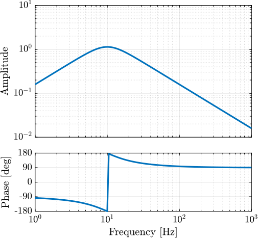

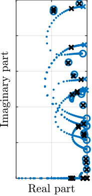
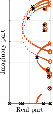
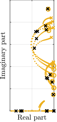
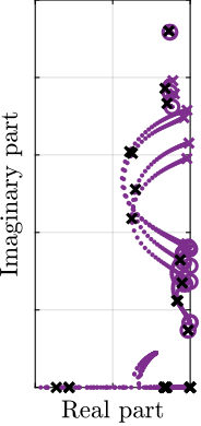
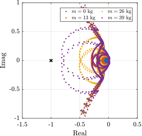
To estimate the added damping, a root-locus plot is computed using the multi-body model (Figure ref:fig:test_id31_iff_root_locus_m0). It can be seen that for all considered payloads, the poles are bounded to the "left-half plane" indicating that the decentralized IFF is robust. The closed-loop poles for the chosen value of the gain are displayed by black crosses. It can be seen that while damping can be added for all payloads (as compared to the open-loop case), the optimal value of the gain is different for each payload. For low payload masses, a higher value of the IFF controller gain could lead to better damping. However, in this study, it was chosen to implement a fix (i.e. non-adaptive) decentralized IFF controller.

Damped Plant

<<ssec:test_id31_iff_perf>>

As the model is accurately modelling the system dynamics, it can be used to estimate the damped plant, i.e. the transfer functions from $\bm{u}^\prime$ to $\bm{\mathcal{L}}$. The obtained damped plants are compared to the open-loop plants in Figure ref:fig:test_id31_comp_ol_iff_plant_model. The peak amplitudes corresponding to the suspension modes are approximately reduced by a factor $10$ for all considered payloads, showing the effectiveness of the decentralized IFF control strategy.

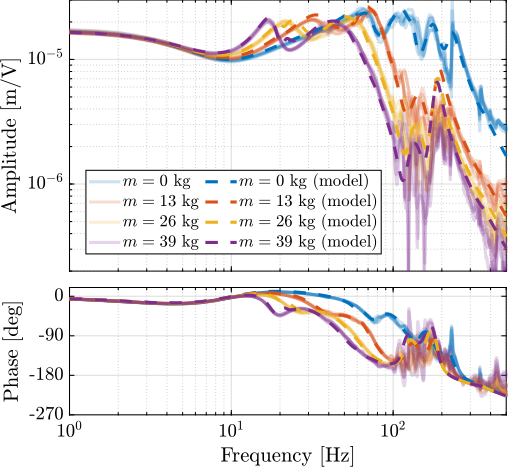
In order to experimentally validate the Decentralized IFF controller, it was implemented and the damped plants (i.e. the transfer function from $\bm{u}^\prime$ to $\bm{\epsilon\mathcal{L}}$) were identified for all payload conditions. The obtained frequency response functions are compared with the model in Figure ref:fig:test_id31_hac_plant_effect_mass verifying the good correlation between the predicted damped plant using the multi-body model and the experimental results.

%% Estimate damped plant from Multi-Body model
Gm_hac_m0_Wz0 = feedback(Gm_m0_Wz0, Kiff, 'name', +1);
Gm_hac_m1_Wz0 = feedback(Gm_m1_Wz0, Kiff, 'name', +1);
Gm_hac_m2_Wz0 = feedback(Gm_m2_Wz0, Kiff, 'name', +1);
Gm_hac_m3_Wz0 = feedback(Gm_m3_Wz0, Kiff, 'name', +1);

% Check Stability
if not(isstable(Gm_hac_m0_Wz0) && isstable(Gm_hac_m1_Wz0) && isstable(Gm_hac_m2_Wz0) && isstable(Gm_hac_m3_Wz0))
    warning("One of the damped system with decentralized IFF is not stable");
end

% The estimated damped plants from the multi-body model are saved
save('./mat/test_id31_simscape_damped_plants.mat', 'Gm_hac_m0_Wz0', 'Gm_hac_m1_Wz0', 'Gm_hac_m2_Wz0', 'Gm_hac_m3_Wz0');

%% Identification of the damped Plant (transfer function from u' to dL)

% Load identification data
data_m0 = load('2023-08-17_17-53_damp_plant_m0_Wz0.mat');
data_m1 = load('2023-08-10_16-01_damp_plant_m1_Wz0.mat');
data_m2 = load('2023-08-10_17-28_damp_plant_m2_Wz0.mat');
data_m3 = load('2023-08-10_18-16_damp_plant_m3_Wz0.mat');

% Hannning Windows
Ts = 1e-4; % Sampling Time [s]
Nfft = floor(2.0/Ts);
win = hanning(Nfft);
Noverlap = floor(Nfft/2);

% And we get the frequency vector
[~, f] = tfestimate(data_m0.uL1.id_plant, data_m0.uL1.e_L1, win, Noverlap, Nfft, 1/Ts);

% Identification without any payload
G_hac_m0_Wz0 = zeros(length(f), 6, 6);
for i_strut = 1:6
    eL = [data_m0.(sprintf("uL%i", i_strut)).e_L1 ; data_m0.(sprintf("uL%i", i_strut)).e_L2 ; data_m0.(sprintf("uL%i", i_strut)).e_L3 ; data_m0.(sprintf("uL%i", i_strut)).e_L4 ; data_m0.(sprintf("uL%i", i_strut)).e_L5 ; data_m0.(sprintf("uL%i", i_strut)).e_L6]';

    G_hac_m0_Wz0(:,:,i_strut) = tfestimate(data_m0.(sprintf("uL%i", i_strut)).id_plant, -detrend(eL, 0), win, Noverlap, Nfft, 1/Ts);
end

% Identification with 1 "payload layer"
G_hac_m1_Wz0 = zeros(length(f), 6, 6);
for i_strut = 1:6
    eL = [data_m1.(sprintf("uL%i", i_strut)).e_L1 ; data_m1.(sprintf("uL%i", i_strut)).e_L2 ; data_m1.(sprintf("uL%i", i_strut)).e_L3 ; data_m1.(sprintf("uL%i", i_strut)).e_L4 ; data_m1.(sprintf("uL%i", i_strut)).e_L5 ; data_m1.(sprintf("uL%i", i_strut)).e_L6]';

    G_hac_m1_Wz0(:,:,i_strut) = tfestimate(data_m1.(sprintf("uL%i", i_strut)).id_plant, -detrend(eL, 0), win, Noverlap, Nfft, 1/Ts);
end

% Identification with 2 "payload layers"
G_hac_m2_Wz0 = zeros(length(f), 6, 6);
for i_strut = 1:6
    eL = [data_m2.(sprintf("uL%i", i_strut)).e_L1 ; data_m2.(sprintf("uL%i", i_strut)).e_L2 ; data_m2.(sprintf("uL%i", i_strut)).e_L3 ; data_m2.(sprintf("uL%i", i_strut)).e_L4 ; data_m2.(sprintf("uL%i", i_strut)).e_L5 ; data_m2.(sprintf("uL%i", i_strut)).e_L6]';

    G_hac_m2_Wz0(:,:,i_strut) = tfestimate(data_m2.(sprintf("uL%i", i_strut)).id_plant, -detrend(eL, 0), win, Noverlap, Nfft, 1/Ts);
end

% Identification with 3 "payload layers"
G_hac_m3_Wz0 = zeros(length(f), 6, 6);
for i_strut = 1:6
    eL = [data_m3.(sprintf("uL%i", i_strut)).e_L1 ; data_m3.(sprintf("uL%i", i_strut)).e_L2 ; data_m3.(sprintf("uL%i", i_strut)).e_L3 ; data_m3.(sprintf("uL%i", i_strut)).e_L4 ; data_m3.(sprintf("uL%i", i_strut)).e_L5 ; data_m3.(sprintf("uL%i", i_strut)).e_L6]';

    G_hac_m3_Wz0(:,:,i_strut) = tfestimate(data_m3.(sprintf("uL%i", i_strut)).id_plant, -detrend(eL, 0), win, Noverlap, Nfft, 1/Ts);
end

% The identified dynamics are then saved for further use.
save('./mat/test_id31_identified_damped_plants.mat', 'G_hac_m0_Wz0', 'G_hac_m1_Wz0', 'G_hac_m2_Wz0', 'G_hac_m3_Wz0', 'f');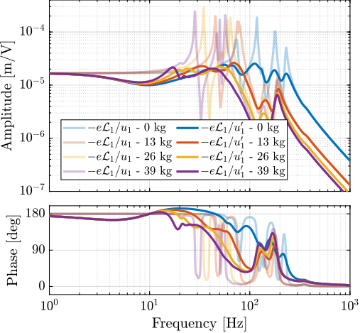

Conclusion

The implementation of a decentralized Integral Force Feedback controller has been successfully demonstrated. Using the multi-body model, the controller was designed and optimized to ensure stability across all payload conditions while providing significant damping of suspension modes. The experimental results validated the model predictions, showing a reduction of peak amplitudes by approximately a factor of 10 across the full payload range (0-39 kg). While higher gains could potentially achieve better damping performance for lighter payloads, the chosen fixed-gain configuration represents a robust compromise that maintains stability and performance across all operating conditions. The good correlation between the modeled and measured damped plants confirms the effectiveness of using the multi-body model for both controller design and performance prediction.

High Authority Control in the frame of the struts

<<sec:test_id31_hac>>

Introduction   ignore

In this section, a High-Authority-Controller is developed to actively stabilize the sample's position. The corresponding control architecture is shown in Figure ref:fig:test_id31_iff_hac_schematic.

As the diagonal terms of the damped plants were found to be all equal (thanks to the system's symmetry and manufacturing and mounting uniformity, see Figure ref:fig:test_id31_hac_plant_effect_mass), a diagonal high authority controller $\bm{K}_{\text{HAC}}$ is implemented with all diagonal terms being equal eqref:eq:eq:test_id31_hac_diagonal.

\begin{equation}\label{eq:eq:test_id31_hac_diagonal} \bm{K}_{\text{HAC}} = K_{\text{HAC}} ⋅ \bm{I}_6 = \begin{bmatrix} K_{\text{HAC}} & & 0
& \ddots &
0 & & K_{\text{HAC}}

\end{bmatrix}

\end{equation}

\begin{tikzpicture}
  % Blocs
  \node[block={2.0cm}{2.0cm}] (P) {Plant};
  \coordinate[] (input)   at ($(P.south west)!0.5!(P.north west)$);
  \coordinate[] (outputH) at ($(P.south east)!0.2!(P.north east)$);
  \coordinate[] (outputL) at ($(P.south east)!0.8!(P.north east)$);

  \node[block, above=0.6 of P] (Klac) {$\bm{K}_\text{IFF}$};
  \node[addb, left= of input] (addF) {};

  \node[block, left= of addF] (Khac) {$\bm{K}_\text{HAC}$};

  % Connections and labels
  \draw[->] (outputL) -- ++(0.6, 0) coordinate(eastlac) |- (Klac.east);
  \node[above right] at (outputL){$\bm{V}_s$};
  \draw[->] (Klac.west) -| (addF.north);
  \draw[->] (addF.east) -- (input) node[above left]{$\bm{u}$};

  \draw[->] (outputH) -- ++(1.6, 0) node[above left]{$\bm{\epsilon\mathcal{L}}$};
  \draw[->] (Khac.east) node[above right]{$\bm{u}^{\prime}$} -- (addF.west);

  \draw[->] ($(outputH) + (1.2, 0)$)node[branch]{} |- ($(Khac.west)+(-0.6, -1.6)$) |- (Khac.west);

  \begin{scope}[on background layer]
    \node[fit={(Klac.north-|eastlac) (addF.west|-P.south)}, fill=black!20!white, draw, dashed, inner sep=10pt] (Pi) {};
    \node[anchor={north west}] at (Pi.north west){$\text{Damped Plant}$};
  \end{scope}
\end{tikzpicture}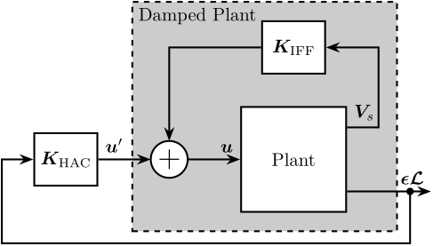

Block diagram of the implemented HAC-IFF controllers. The controller $\bm{K}_{\text{HAC}}$ is a diagonal controller with the same elements on every diagonal term $K_{\text{HAC}}$.

Damped Plant

<<ssec:test_id31_iff_hac_plant>>

To verify whether the multi body model accurately represents the measured damped dynamics, both direct terms and coupling terms corresponding to the first actuator are compared in Figure ref:fig:test_id31_comp_simscape_hac. Considering the complexity of the system's dynamics, the model can be considered to well represent the system's dynamics, and can therefore be used to tune the feedback controller and evaluate its performances.

% Load the estimated damped plant from the multi-body model
load('test_id31_simscape_damped_plants.mat', 'Gm_hac_m0_Wz0', 'Gm_hac_m1_Wz0', 'Gm_hac_m2_Wz0', 'Gm_hac_m3_Wz0');
% Load the measured damped plants
load('test_id31_identified_damped_plants.mat', 'G_hac_m0_Wz0', 'G_hac_m1_Wz0', 'G_hac_m2_Wz0', 'G_hac_m3_Wz0', 'f');
% Load the undamped plant for comparison
load('test_id31_identified_open_loop_plants.mat', 'G_int_m0_Wz0', 'G_int_m1_Wz0', 'G_int_m2_Wz0', 'G_int_m3_Wz0', 'f');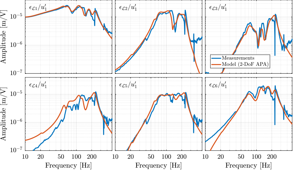

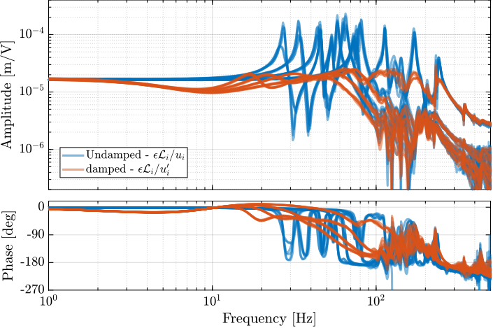
Comparison of the measured (in blue) and modeled (in red) frequency transfer functions from the first control signal ($u_1^\prime$) of the damped plant to the estimated errors ($\epsilon_{\mathcal{L}_i}$) in the frame of the six struts by the external metrology

The challenge here is to tune an high authority controller such that it is robust to the change of dynamics due to different payloads being used. Doing that without using the HAC-LAC strategy would require to design a controller which gives good performances for all the undamped dynamics (blue curves in Figure ref:fig:test_id31_comp_all_undamped_damped_plants), which is a very complex control problem. With the HAC-LAC strategy, the designed controller instead has to be be robust to all the damped dynamics (red curves in Figure ref:fig:test_id31_comp_all_undamped_damped_plants), which is easier from a control perspective. This is one of the key benefit of using the HAC-LAC strategy.

Comparison of the (six) direct terms for all (four) payload conditions in the undamped case (in blue) and the damped case (i.e. with the decentralized IFF being implemented, in red).

Interaction Analysis

<<sec:test_id31_hac_interaction_analysis>>

As the control strategy here is to apply a diagonal control in the frame of the struts, it is important to determine the frequency at which multivariable effects become significant, as this represents a critical limitation of the control approach. To conduct this interaction analysis, the acrfull:rga $\bm{\Lambda_G}$ is first computed using eqref:eq:test_id31_rga for the plant dynamics identified with the multiple payload masses.

\begin{equation}\label{eq:test_id31_rga} \bm{Λ_G}(ω) = \bm{G}(jω) ⋆ ≤ft(\bm{G}(jω)^-1\right)^T, \quad (⋆ \text{ means element wise multiplication})

\end{equation}

Then, acrshort:rga numbers are computed using eqref:eq:test_id31_rga_number and are use as a metric for interaction cite:&skogestad07_multiv_feedb_contr chapt. 3.4.

\begin{equation}\label{eq:test_id31_rga_number} \text{RGA number}(ω) = \|\bm{Λ_G}(ω) - \bm{I}\|_{\text{sum}}

\end{equation}

The obtained acrshort:rga numbers are compared in Figure ref:fig:test_id31_hac_rga_number. The results indicates that higher payload masses increase the coupling when implementing control in the strut reference frame (i.e., decentralized approach). This indicates that it is progressively more challenging to achieve high bandwidth performance as the payload mass increases. This behavior can be attributed to the fundamental approach of implementing control in the frame of the struts. Indeed, above the suspension modes of the nano-hexapod, the induced motion by the piezoelectric actuators is no longer dictated by the kinematics but rather by the inertia of the different parts. This design choice, while beneficial for system simplicity, introduces inherent limitations in the system's ability to handle larger masses at high frequency.

%% Interaction Analysis - RGA Number
rga_m0 = zeros(1,size(G_hac_m0_Wz0,1));
for i = 1:length(rga_m0)
    rga_m0(i) = sum(sum(abs(inv(squeeze(G_hac_m0_Wz0(i,:,:)).').*squeeze(G_hac_m0_Wz0(i,:,:)) - eye(6))));
end

rga_m1 = zeros(1,size(G_hac_m1_Wz0,1));
for i = 1:length(rga_m1)
    rga_m1(i) = sum(sum(abs(inv(squeeze(G_hac_m1_Wz0(i,:,:)).').*squeeze(G_hac_m1_Wz0(i,:,:)) - eye(6))));
end

rga_m2 = zeros(1,size(G_hac_m2_Wz0,1));
for i = 1:length(rga_m2)
    rga_m2(i) = sum(sum(abs(inv(squeeze(G_hac_m2_Wz0(i,:,:)).').*squeeze(G_hac_m2_Wz0(i,:,:)) - eye(6))));
end

rga_m3 = zeros(1,size(G_hac_m3_Wz0,1));
for i = 1:length(rga_m3)
    rga_m3(i) = sum(sum(abs(inv(squeeze(G_hac_m3_Wz0(i,:,:)).').*squeeze(G_hac_m3_Wz0(i,:,:)) - eye(6))));
end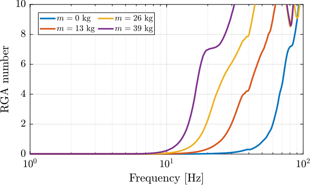

RGA-number for the damped plants - Comparison of all the payload conditions

Robust Controller Design

<<ssec:test_id31_iff_hac_controller>>

A diagonal controller was designed to be robust to change of payloads, which means that every damped plants shown in Figure ref:fig:test_id31_comp_all_undamped_damped_plants should be considered during the controller design. For this controller design, a crossover frequency of $5\,\text{Hz}$ was chosen to limit multivariable effects as explain in Section ref:sec:test_id31_hac_interaction_analysis. One integrator is added to increase the low frequency gain, a lead is added around $5\,\text{Hz}$ to increase the stability margins and a first order low pass filter with a cut-off frequency of $30\,\text{Hz}$ is added to improve the robustness to dynamical uncertainty at high frequency. The controller transfer function is shown in eqref:eq:test_id31_robust_hac.

\begin{equation}\label{eq:test_id31_robust_hac} K_{\text{HAC}}(s) = g_0 ⋅ _brace{\frac{ω_c}{s}}_{\text{int}} ⋅ _brace{\frac{1}{\sqrt{α}}\frac{1 + \frac{s}{ω_c/\sqrt{α}}}{1 + \frac{s}{ω_c\sqrt{α}}}}_{\text{lead}} ⋅ _brace{\frac{1}{1 + \frac{s}{ω_0}}}_{\text{LPF}}, \quad ≤ft( ω_c = 2π5\,\text{rad/s},\ α = 2,\ ω_0 = 2π30\,\text{rad/s} \right)

\end{equation}

The obtained "decentralized" loop-gains (i.e. the diagonal element of the controller times the diagonal terms of the plant) are shown in Figure ref:fig:test_id31_hac_loop_gain. Closed-loop stability is verified by computing the characteristic Loci (Figure ref:fig:test_id31_hac_characteristic_loci). However, small stability margins are observed for the highest mass, indicating that some multivariable effects are in play.

%% HAC Design
% Wanted crossover
wc = 2*pi*5; % [rad/s]

% Integrator
H_int = wc/s;

% Lead to increase phase margin
a  = 2;  % Amount of phase lead / width of the phase lead / high frequency gain
H_lead = 1/sqrt(a)*(1 + s/(wc/sqrt(a)))/(1 + s/(wc*sqrt(a)));

% Low Pass filter to increase robustness
H_lpf = 1/(1 + s/2/pi/30);

% Gain to have unitary crossover at 5Hz
[~, i_f] = min(abs(f - wc/2/pi));
H_gain = 1./abs(G_hac_m0_Wz0(i_f, 1, 1));

% Decentralized HAC
Khac = H_gain  * ... % Gain
       H_int   * ... % Integrator
       H_lpf   * ... % Low Pass filter
       eye(6);       % 6x6 Diagonal

% The designed HAC controller is saved
save('./mat/test_id31_K_hac_robust.mat', 'Khac');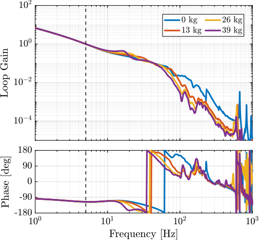

Performance estimation with simulation of Tomography scans

<<ssec:test_id31_iff_hac_perf>>

To estimate the performances that can be expected with this HAC-LAC architecture and the designed controller, simulations of tomography experiments were performed⁵. The rotational velocity was set to $180\,\text{deg/s}$, and no payload was added on top of the nano-hexapod. An open-loop simulation and a closed-loop simulation were performed and compared in Figure ref:fig:test_id31_tomo_m0_30rpm_robust_hac_iff_sim. The obtained closed-loop positioning accuracy was found to comply with the requirements as it succeeded to keep the point of interest on the beam (Figure ref:fig:test_id31_tomo_m0_30rpm_robust_hac_iff_sim_yz).

%% Tomography experiment
% Sample is not centered with the rotation axis
% This is done by offsetfing the micro-hexapod by 0.9um
P_micro_hexapod = [2.5e-6; 0; -0.3e-6]; % [m]

open(mdl);
set_param(mdl, 'StopTime', '3'); % 6 turns at 180deg/s (30rpm)

initializeGround();
initializeGranite();
initializeTy();
initializeRy();
initializeRz();
initializeMicroHexapod('AP', P_micro_hexapod);
initializeNanoHexapod('flex_bot_type', '2dof', ...
                      'flex_top_type', '3dof', ...
                      'motion_sensor_type', 'plates', ...
                      'actuator_type', '2dof');
initializeSample('type', '0');

initializeSimscapeConfiguration('gravity', false);
initializeLoggingConfiguration('log', 'all', 'Ts', 1e-4);
initializeController('type', 'open-loop');

initializeDisturbances(...
    'Dw_x',  true, ... % Ground Motion - X direction
    'Dw_y',  true, ... % Ground Motion - Y direction
    'Dw_z',  true, ... % Ground Motion - Z direction
    'Fdy_x', false, ... % Translation Stage - X direction
    'Fdy_z', false, ... % Translation Stage - Z direction
    'Frz_x', true, ... % Spindle - X direction
    'Frz_y', true, ... % Spindle - Y direction
    'Frz_z', true);    % Spindle - Z direction

initializeReferences(...
    'Rz_type', 'rotating', ...
    'Rz_period', 360/180, ... % 180deg/s, 30rpm
    'Dh_pos', [P_micro_hexapod; 0; 0; 0]);

% Open-Loop Simulation
sim(mdl);
exp_tomo_ol_m0_Wz180 = simout;

% Closed-Loop Simulation
load('test_id31_K_iff.mat', 'Kiff');
load('test_id31_K_hac_robust.mat', 'Khac');
initializeController('type', 'hac-iff');
initializeSample('type', '0');
sim(mdl);
exp_tomo_cl_m0_Wz180 = simout;

% Save the simulation results
save('./mat/test_id31_exp_tomo_ol_cl_30rpm_sim.mat', 'exp_tomo_ol_m0_Wz180', 'exp_tomo_cl_m0_Wz180');

% Load the simulation results
load('test_id31_exp_tomo_ol_cl_30rpm_sim.mat', 'exp_tomo_ol_m0_Wz180', 'exp_tomo_cl_m0_Wz180');

Robustness estimation with simulation of Tomography scans

<<ssec:test_id31_iff_hac_robustness>>

To verify the robustness to the change of payload mass, four simulations of tomography experiments were performed with payloads as shown Figure ref:fig:test_id31_picture_masses (i.e. $0\,kg$, $13\,kg$, $26\,kg$ and $39\,kg$). This time, the rotational velocity was set at $6\,\text{deg/s}$, as it is the typical rotational velocity for heavy samples.

The closed-loop systems were stable for all payload conditions, indicating good control robustness. However, the positioning errors are getting worse as the payload mass increases, especially in the lateral $D_y$ direction, as shown in Figure ref:fig:test_id31_hac_tomography_Wz36_simulation. Yet it was decided that this controller will be tested experimentally, and improved if necessary.

%% Simulation of tomography experiments at 1RPM with all payloads
% Configuration
open(mdl);
set_param(mdl, 'StopTime', '2'); % 30 degrees at 1rpm
initializeLoggingConfiguration('log', 'all', 'Ts', 1e-3);
initializeController('type', 'hac-iff');
initializeReferences(...
    'Rz_type', 'rotating', ...
    'Rz_period', 360/6, ... % 6deg/s, 1 rpm
    'Dh_pos', [P_micro_hexapod; 0; 0; 0]);

% Perform the simulations
initializeSample('type', '0');
sim(mdl);
exp_tomo_cl_m0_1rpm = simout;
initializeSample('type', '1');
sim(mdl);
exp_tomo_cl_m1_1rpm = simout;
initializeSample('type', '2');
sim(mdl);
exp_tomo_cl_m2_1rpm = simout;
initializeSample('type', '3');
sim(mdl);
exp_tomo_cl_m3_1rpm = simout;

% Save the simulation results
save('./mat/test_id31_exp_tomo_cl_1rpm_sim.mat', 'exp_tomo_cl_m0_1rpm', 'exp_tomo_cl_m1_1rpm', 'exp_tomo_cl_m2_1rpm', 'exp_tomo_cl_m3_1rpm');

% Load the simulation results
load('test_id31_exp_tomo_cl_1rpm_sim.mat', 'exp_tomo_cl_m0_1rpm', 'exp_tomo_cl_m1_1rpm', 'exp_tomo_cl_m2_1rpm', 'exp_tomo_cl_m3_1rpm');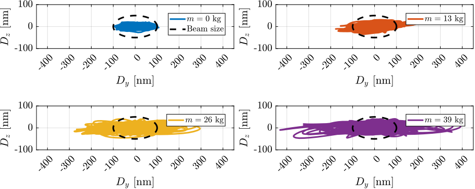

Positioning errors in the Y-Z plane during tomography experiments simulated using the multi-body model (in closed-loop)

Conclusion

In this section, a High-Authority-Controller was developed to actively stabilize the sample's position. The multi-body model was first validated by comparing it with measured frequency responses of the damped plant, showing good agreement for both direct terms and coupling terms. This validation confirmed that the model could be reliably used to tune the feedback controller and evaluate its performances.

An interaction analysis using the RGA-number was then performed, revealing that higher payload masses lead to increased coupling when implementing control in the strut reference frame. Based on this analysis, a diagonal controller with a crossover frequency of 5 Hz was designed, incorporating an integrator, a lead compensator, and a first order low-pass filter.

Finally, simulations of tomography experiments were performed to validate the HAC-LAC architecture. The closed-loop system remained stable for all tested payload conditions (0 to 39 kg). With no payload at $180\,\text{deg/s}$, the NASS successfully kept the sample point of interested on the beam, which fulfills the specifications. At $6\,\text{deg/s}$, while positioning errors increased with the payload mass (particularly in the lateral direction), the system maintained stable. These results demonstrate both the effectiveness and limitations of implementing control in the frame of the struts.

Validation with Scientific experiments

<<sec:test_id31_experiments>>

Introduction   ignore

In this section, the goal is to evaluate the performances of the NASS and validate its use for typical scientific experiments. However, the online metrology prototype (presented in Section ref:sec:test_id31_metrology) does not allow samples to be placed on top of the nano-hexapod while being illuminated by the x-ray beam. Nevertheless, in order to fully validate the NASS, typical motion performed during scientific experiments can be mimicked, and the positioning performances can be evaluated.

Several scientific experiments are here replicated, such as:

• Tomography scans: continuous rotation of the Spindle along the vertical axis (Section ref:ssec:test_id31_scans_tomography)
• Reflectivity scans: $R_y$ rotations using the tilt-stage (Section ref:ssec:test_id31_scans_reflectivity)
• Vertical layer scans: $D_z$ step motion or ramp scans using the nano-hexapod (Section ref:ssec:test_id31_scans_dz)
• Lateral scans: $D_y$ scans using the $T_y$ translation stage (Section ref:ssec:test_id31_scans_dy)
• Diffraction Tomography:continuous $R_z$ rotation using the Spindle and lateral $D_y$ scans performed at the same time using the translation stage. This is the experiment with the most stringent requirements (Section ref:ssec:test_id31_scans_diffraction_tomo)

Unless explicitly stated, all the closed-loop experiments are performed using the robust (i.e. conservative) high authority controller designed in Section ref:ssec:test_id31_iff_hac_controller.

For each experiment, the obtained performances are compared to the specifications for the most depending case in which nano-focusing optics are used to focus the beam down to $200\,nm\times 100\,nm$. In this case, the goal is to keep the sample's point of interested in the beam, and therefore the $D_y$ and $D_z$ positioning errors should be less than $200\,nm$ and $100\,nm$ peak-to-peak respectively. The $R_y$ error should be less than $1.7\,\mu\text{rad}$ peak-to-peak. In terms of RMS errors, this corresponds to $30\,nm$ in $D_y$, $15\,nm$ in $D_z$ and $250\,\text{nrad}$ in $R_y$ (a summary of the specifications is given in Table ref:tab:test_id31_experiments_specifications).

Results obtained for all the experiments are summarized and compared to the specifications in Section ref:ssec:test_id31_scans_conclusion.

	$D_y$	$D_z$	$R_y$
peak 2 peak	200nm	100nm	$1.7\,\mu\text{rad}$
RMS	30nm	15nm	$250\,\text{nrad}$

Tomography Scans

<<ssec:test_id31_scans_tomography>>

Slow Tomography scans

First, tomography scans are performed with a rotational velocity of $6\,\text{deg/s}$ for all considered payload masses (shown in Figure ref:fig:test_id31_picture_masses). Each experimental sequence consisted of two complete spindle rotations: an initial open-loop rotation followed by a closed-loop rotation. The experimental results for the $26\,\text{kg}$ payload are presented in Figure ref:fig:test_id31_tomo_m2_1rpm_robust_hac_iff_fit.

Due to static deformation of the micro-station stages under payload loading, a significant eccentricity was observed between the point of interest and the spindle rotation axis. To establish a theoretical lower bound for open-loop errors, an ideal scenario was assumed where the point of interest perfectly aligns with the spindle rotation axis. This idealized case was simulated by first calculating the eccentricity through circular fitting (represented by the dashed black circle in Figure ref:fig:test_id31_tomo_m2_1rpm_robust_hac_iff_fit), and then subtracting it from the measured data, as shown in Figure ref:fig:test_id31_tomo_m2_1rpm_robust_hac_iff_fit_removed. While this approach likely underestimates actual open-loop errors, as perfect alignment is practically unattainable, it enables a more balanced comparison with closed-loop performance.

%% Load Tomography scans with robust controller
data_tomo_m0_Wz6 = load("2023-08-11_11-37_tomography_1rpm_m0.mat");
data_tomo_m0_Wz6.time = Ts*[0:length(data_tomo_m0_Wz6.Rz)-1];

data_tomo_m1_Wz6 = load("2023-08-11_11-15_tomography_1rpm_m1.mat");
data_tomo_m1_Wz6.time = Ts*[0:length(data_tomo_m1_Wz6.Rz)-1];

data_tomo_m2_Wz6 = load("2023-08-11_10-59_tomography_1rpm_m2.mat");
data_tomo_m2_Wz6.time = Ts*[0:length(data_tomo_m2_Wz6.Rz)-1];

data_tomo_m3_Wz6 = load("2023-08-11_10-24_tomography_1rpm_m3.mat");
data_tomo_m3_Wz6.time = Ts*[0:length(data_tomo_m3_Wz6.Rz)-1];

%% Find best circle fit for all experiments
[~, i_m0] = find(data_tomo_m0_Wz6.hac_status == 1);
[x_m0, y_m0, R_m0] = circlefit(data_tomo_m0_Wz6.Dx_int(1:i_m0), data_tomo_m0_Wz6.Dy_int(1:i_m0));
fun = @(theta)rms((data_tomo_m0_Wz6.Dx_int(1:i_m0) - (x_m0 + R_m0*cos(data_tomo_m0_Wz6.Rz(1:i_m0)+theta(1)))).^2 + ...
                  (data_tomo_m0_Wz6.Dy_int(1:i_m0) - (y_m0 + R_m0*sin(data_tomo_m0_Wz6.Rz(1:i_m0)+theta(1)))).^2);
delta_theta_m0 = fminsearch(fun, 0);

[~, i_m1] = find(data_tomo_m1_Wz6.hac_status == 1);
[x_m1, y_m1, R_m1] = circlefit(data_tomo_m1_Wz6.Dx_int(1:i_m1), data_tomo_m1_Wz6.Dy_int(1:i_m1));
fun = @(theta)rms((data_tomo_m1_Wz6.Dx_int(1:i_m1) - (x_m1 + R_m1*cos(data_tomo_m1_Wz6.Rz(1:i_m1)+theta(1)))).^2 + ...
                  (data_tomo_m1_Wz6.Dy_int(1:i_m1) - (y_m1 + R_m1*sin(data_tomo_m1_Wz6.Rz(1:i_m1)+theta(1)))).^2);
delta_theta_m1 = fminsearch(fun, 0);

[~, i_m2] = find(data_tomo_m2_Wz6.hac_status == 1);
[x_m2, y_m2, R_m2] = circlefit(data_tomo_m2_Wz6.Dx_int(1:i_m2), data_tomo_m2_Wz6.Dy_int(1:i_m2));
fun = @(theta)rms((data_tomo_m2_Wz6.Dx_int(1:i_m2) - (x_m2 + R_m2*cos(data_tomo_m2_Wz6.Rz(1:i_m2)+theta(1)))).^2 + ...
                  (data_tomo_m2_Wz6.Dy_int(1:i_m2) - (y_m2 + R_m2*sin(data_tomo_m2_Wz6.Rz(1:i_m2)+theta(1)))).^2);
delta_theta_m2 = fminsearch(fun, 0);

[~, i_m3] = find(data_tomo_m3_Wz6.hac_status == 1);
[x_m3, y_m3, R_m3] = circlefit(data_tomo_m3_Wz6.Dx_int(1:i_m3), data_tomo_m3_Wz6.Dy_int(1:i_m3));
fun = @(theta)rms((data_tomo_m3_Wz6.Dx_int(1:i_m3) - (x_m3 + R_m3*cos(data_tomo_m3_Wz6.Rz(1:i_m3)+theta(1)))).^2 + ...
                  (data_tomo_m3_Wz6.Dy_int(1:i_m3) - (y_m3 + R_m3*sin(data_tomo_m3_Wz6.Rz(1:i_m3)+theta(1)))).^2);
delta_theta_m3 = fminsearch(fun, 0);

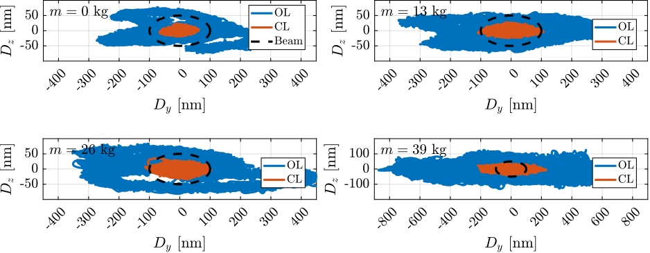
After eccentricity compensation for each experiment, the residual motion in the $Y-Z$ is compared against the minimum beam size, as illustrated in Figure ref:fig:test_id31_tomo_Wz36_results. Results are indicating the NASS succeeds in keeping the sample's point of interests on the beam, except for the highest mass of $39\,\text{kg}$ for which the lateral motion is a bit too high. These experimental findings align with the predictions from the tomography simulations presented in Section ref:ssec:test_id31_iff_hac_robustness.

Measured errors in the $Y-Z$ plane during tomography experiments at $6\,\text{deg/s}$ for all considered payloads. In the open-loop case, the effect of eccentricity is removed from the data.

%% Estimate RMS of the errors while in closed-loop and open-loop - Tomography at 6deg/s
% No mass
data_tomo_m0_Wz6.Dy_rms_cl = rms(detrend(data_tomo_m0_Wz6.Dy_int(i_m0+1e4:end), 0));
data_tomo_m0_Wz6.Dz_rms_cl = rms(detrend(data_tomo_m0_Wz6.Dz_int(i_m0+1e4:end), 0));
data_tomo_m0_Wz6.Ry_rms_cl = rms(detrend(data_tomo_m0_Wz6.Ry_int(i_m0+1e4:end), 0));

% Remove eccentricity for OL errors
data_tomo_m0_Wz6.Dy_rms_ol = rms(data_tomo_m0_Wz6.Dy_int(1:i_m0) - (y_m0 + R_m0*sin(data_tomo_m0_Wz6.Rz(1:i_m0)+delta_theta_m0)));
data_tomo_m0_Wz6.Dz_rms_ol = rms(detrend(data_tomo_m0_Wz6.Dz_int(1:i_m0), 0));
[x0, y0, R] = circlefit(data_tomo_m0_Wz6.Rx_int(1:i_m0), data_tomo_m0_Wz6.Ry_int(1:i_m0));
fun = @(theta)rms((data_tomo_m0_Wz6.Rx_int(1:i_m0) - (x0 + R*cos(data_tomo_m0_Wz6.Rz(1:i_m0)+theta(1)))).^2 + ...
                  (data_tomo_m0_Wz6.Ry_int(1:i_m0) - (y0 + R*sin(data_tomo_m0_Wz6.Rz(1:i_m0)+theta(1)))).^2);
delta_theta = fminsearch(fun, 0);
data_tomo_m0_Wz6.Ry_rms_ol = rms(data_tomo_m0_Wz6.Ry_int(1:i_m0) - (y0 + R*sin(data_tomo_m0_Wz6.Rz(1:i_m0)+delta_theta)));

% 1 "layer mass"
data_tomo_m1_Wz6.Dy_rms_cl = rms(detrend(data_tomo_m1_Wz6.Dy_int(i_m1+1e4:end), 0));
data_tomo_m1_Wz6.Dz_rms_cl = rms(detrend(data_tomo_m1_Wz6.Dz_int(i_m1+1e4:end), 0));
data_tomo_m1_Wz6.Ry_rms_cl = rms(detrend(data_tomo_m1_Wz6.Ry_int(i_m1+1e4:end), 0));

% Remove eccentricity for OL errors
data_tomo_m1_Wz6.Dy_rms_ol = rms(data_tomo_m1_Wz6.Dy_int(1:i_m1) - (y_m1 + R_m1*sin(data_tomo_m1_Wz6.Rz(1:i_m1)+delta_theta_m1)));
data_tomo_m1_Wz6.Dz_rms_ol = rms(detrend(data_tomo_m1_Wz6.Dz_int(1:i_m1), 0));
[x0, y0, R] = circlefit(data_tomo_m1_Wz6.Rx_int(1:i_m1), data_tomo_m1_Wz6.Ry_int(1:i_m1));
fun = @(theta)rms((data_tomo_m1_Wz6.Rx_int(1:i_m1) - (x0 + R*cos(data_tomo_m1_Wz6.Rz(1:i_m1)+theta(1)))).^2 + ...
                  (data_tomo_m1_Wz6.Ry_int(1:i_m1) - (y0 + R*sin(data_tomo_m1_Wz6.Rz(1:i_m1)+theta(1)))).^2);
delta_theta = fminsearch(fun, 0);
data_tomo_m1_Wz6.Ry_rms_ol = rms(data_tomo_m1_Wz6.Ry_int(1:i_m1) - (y0 + R*sin(data_tomo_m1_Wz6.Rz(1:i_m1)+delta_theta)));

% 2 "layer masses"
data_tomo_m2_Wz6.Dy_rms_cl = rms(detrend(data_tomo_m2_Wz6.Dy_int(i_m2+1e4:end), 0));
data_tomo_m2_Wz6.Dz_rms_cl = rms(detrend(data_tomo_m2_Wz6.Dz_int(i_m2+1e4:end), 0));
data_tomo_m2_Wz6.Ry_rms_cl = rms(detrend(data_tomo_m2_Wz6.Ry_int(i_m2+1e4:end), 0));

% Remove eccentricity for OL errors
data_tomo_m2_Wz6.Dy_rms_ol = rms(data_tomo_m2_Wz6.Dy_int(1:i_m2) - (y_m2 + R_m2*sin(data_tomo_m2_Wz6.Rz(1:i_m2)+delta_theta_m2)));
data_tomo_m2_Wz6.Dz_rms_ol = rms(detrend(data_tomo_m2_Wz6.Dz_int(1:i_m2), 0));
[x0, y0, R] = circlefit(data_tomo_m2_Wz6.Rx_int(1:i_m2), data_tomo_m2_Wz6.Ry_int(1:i_m2));
fun = @(theta)rms((data_tomo_m2_Wz6.Rx_int(1:i_m2) - (x0 + R*cos(data_tomo_m2_Wz6.Rz(1:i_m2)+theta(1)))).^2 + ...
                  (data_tomo_m2_Wz6.Ry_int(1:i_m2) - (y0 + R*sin(data_tomo_m2_Wz6.Rz(1:i_m2)+theta(1)))).^2);
delta_theta = fminsearch(fun, 0);
data_tomo_m2_Wz6.Ry_rms_ol = rms(data_tomo_m2_Wz6.Ry_int(1:i_m2) - (y0 + R*sin(data_tomo_m2_Wz6.Rz(1:i_m2)+delta_theta)));

% 3 "layer masses"
data_tomo_m3_Wz6.Dy_rms_cl = rms(detrend(data_tomo_m3_Wz6.Dy_int(i_m3+1e4:end), 0));
data_tomo_m3_Wz6.Dz_rms_cl = rms(detrend(data_tomo_m3_Wz6.Dz_int(i_m3+1e4:end), 0));
data_tomo_m3_Wz6.Ry_rms_cl = rms(detrend(data_tomo_m3_Wz6.Ry_int(i_m3+1e4:end), 0));

% Remove eccentricity for OL errors
data_tomo_m3_Wz6.Dy_rms_ol = rms(data_tomo_m3_Wz6.Dy_int(1:i_m3) - (y_m3 + R_m3*sin(data_tomo_m3_Wz6.Rz(1:i_m3)+delta_theta_m3)));
data_tomo_m3_Wz6.Dz_rms_ol = rms(detrend(data_tomo_m3_Wz6.Dz_int(1:i_m3), 0));
[x0, y0, R] = circlefit(data_tomo_m3_Wz6.Rx_int(1:i_m3), data_tomo_m3_Wz6.Ry_int(1:i_m3));
fun = @(theta)rms((data_tomo_m3_Wz6.Rx_int(1:i_m3) - (x0 + R*cos(data_tomo_m3_Wz6.Rz(1:i_m3)+theta(1)))).^2 + ...
                  (data_tomo_m3_Wz6.Ry_int(1:i_m3) - (y0 + R*sin(data_tomo_m3_Wz6.Rz(1:i_m3)+theta(1)))).^2);
delta_theta = fminsearch(fun, 0);
data_tomo_m3_Wz6.Ry_rms_ol = rms(data_tomo_m3_Wz6.Ry_int(1:i_m3) - (y0 + R*sin(data_tomo_m3_Wz6.Rz(1:i_m3)+delta_theta)));

Fast Tomography scans

A tomography experiment was then performed with the highest rotational velocity of the Spindle: $180\,\text{deg/s}$⁶. The trajectory of the point of interest during this fast tomography scan is shown in Figure ref:fig:test_id31_tomo_m0_30rpm_robust_hac_iff_exp. While the experimental results closely mirror the simulation results (Figure ref:fig:test_id31_tomo_m0_30rpm_robust_hac_iff_sim), the actual performance are slightly lower than predicted. Nevertheless, even with this robust (conservative) HAC implementation, the system performance approaches the specified requirements.

%% Experimental Results for Tomography at 180deg/s, no payload
data_tomo_m0_Wz180 = load('2023-08-17_15-26_tomography_30rpm_m0_robust.mat');

[~, i_m0] = find(data_tomo_m0_Wz180.hac_status == 1);
[x_m0, y_m0, R_m0] = circlefit(data_tomo_m0_Wz180.Dx_int(1:i_m0), data_tomo_m0_Wz180.Dy_int(1:i_m0));
fun = @(theta)rms((data_tomo_m0_Wz180.Dx_int(1:i_m0) - (x_m0 + R_m0*cos(data_tomo_m0_Wz180.Rz(1:i_m0)+theta(1)))).^2 + ...
                  (data_tomo_m0_Wz180.Dy_int(1:i_m0) - (y_m0 + R_m0*sin(data_tomo_m0_Wz180.Rz(1:i_m0)+theta(1)))).^2);
delta_theta_m0 = fminsearch(fun, 0);

%% Estimate RMS of the errors while in closed-loop and open-loop - Tomography at 180deg/s
% No mass
data_tomo_m0_Wz180.Dy_rms_cl = rms(detrend(data_tomo_m0_Wz180.Dy_int(i_m0+1e4:end), 0));
data_tomo_m0_Wz180.Dz_rms_cl = rms(detrend(data_tomo_m0_Wz180.Dz_int(i_m0+1e4:end), 0));
data_tomo_m0_Wz180.Ry_rms_cl = rms(detrend(data_tomo_m0_Wz180.Ry_int(i_m0+1e4:end), 0));

% Remove eccentricity for OL errors
data_tomo_m0_Wz180.Dy_rms_ol = rms(data_tomo_m0_Wz180.Dy_int(1:i_m0) - (y_m0 + R_m0*sin(data_tomo_m0_Wz180.Rz(1:i_m0)+delta_theta_m0)));
data_tomo_m0_Wz180.Dz_rms_ol = rms(detrend(data_tomo_m0_Wz180.Dz_int(1:i_m0), 0));
[x0, y0, R] = circlefit(data_tomo_m0_Wz180.Rx_int(1:i_m0), data_tomo_m0_Wz180.Ry_int(1:i_m0));
fun = @(theta)rms((data_tomo_m0_Wz180.Rx_int(1:i_m0) - (x0 + R*cos(data_tomo_m0_Wz180.Rz(1:i_m0)+theta(1)))).^2 + ...
                  (data_tomo_m0_Wz180.Ry_int(1:i_m0) - (y0 + R*sin(data_tomo_m0_Wz180.Rz(1:i_m0)+theta(1)))).^2);
delta_theta = fminsearch(fun, 0);
data_tomo_m0_Wz180.Ry_rms_ol = rms(data_tomo_m0_Wz180.Ry_int(1:i_m0) - (y0 + R*sin(data_tomo_m0_Wz180.Rz(1:i_m0)+delta_theta)));

Cumulative Amplitude Spectra

A comparative analysis was conducted using three tomography scans at $180,\text{deg/s}$ to evaluate the effectiveness of the HAC-LAC strategy in reducing positioning errors. The scans were performed under three conditions: open-loop, with decentralized IFF control, and with the complete HAC-LAC strategy. For these specific measurements, an enhanced high authority controller was optimized for low payload masses to meet performance requirements.

Figure ref:fig:test_id31_hac_cas_cl presents the cumulative amplitude spectra of the position errors for all three cases. The results reveal two distinct control contributions: the decentralized IFF effectively attenuates vibrations near the nano-hexapod suspension modes (an achievement not possible with HAC alone), while the high authority controller suppresses low-frequency vibrations primarily arising from Spindle guiding errors. Notably, the spectral patterns in Figure ref:fig:test_id31_hac_cas_cl closely resemble the cumulative amplitude spectra computed in the project's early stages.

This experiment also illustrates that when needed, performance can be enhanced by designing controllers for specific experimental conditions, rather than relying solely on robust controllers that accommodate all payload ranges.

%% Jacobian to compute the motion in the X-Y-Z-Rx-Ry directions
J_int_to_X = [ 0                 0                -0.787401574803149 -0.212598425196851  0;
               0.78740157480315  0.21259842519685  0                  0                  0;
               0                 0                 0                  0                 -1;
             -13.1233595800525  13.1233595800525   0                  0                  0;
               0                 0               -13.1233595800525   13.1233595800525    0];

%% Parameters for frequency analysis computation
Nfft = floor(20.0/Ts);
win = hanning(Nfft);
Noverlap = floor(Nfft/2);

%% Open-Loop measurement
data_ol_Wz180 = load('2023-08-11_16-51_m0_lac_off.mat'); % no rotation

a = J_int_to_X*[data_ol_Wz180.d1; data_ol_Wz180.d2; data_ol_Wz180.d3; data_ol_Wz180.d4; data_ol_Wz180.d5];
data_ol_Wz180.Dx_int = a(1,:);
data_ol_Wz180.Dy_int = a(2,:);
data_ol_Wz180.Dz_int = a(3,:);
data_ol_Wz180.Rx_int = a(4,:);
data_ol_Wz180.Ry_int = a(5,:);

[data_ol_Wz180.pxx_Dx, data_ol_Wz180.f] = pwelch(detrend(data_ol_Wz180.Dx_int, 0), win, Noverlap, Nfft, 1/Ts);
[data_ol_Wz180.pxx_Dy, ~              ] = pwelch(detrend(data_ol_Wz180.Dy_int, 0), win, Noverlap, Nfft, 1/Ts);
[data_ol_Wz180.pxx_Dz, ~              ] = pwelch(detrend(data_ol_Wz180.Dz_int, 0), win, Noverlap, Nfft, 1/Ts);
[data_ol_Wz180.pxx_Rx, ~              ] = pwelch(detrend(data_ol_Wz180.Rx_int, 0), win, Noverlap, Nfft, 1/Ts);
[data_ol_Wz180.pxx_Ry, ~              ] = pwelch(detrend(data_ol_Wz180.Ry_int, 0), win, Noverlap, Nfft, 1/Ts);

%% Effect of LAC - 180 deg/s
data_lac_Wz180 = load('2023-08-11_17-36_m0_lac_on_30rpm.mat');

a = J_int_to_X*[data_lac_Wz180.d1; data_lac_Wz180.d2; data_lac_Wz180.d3; data_lac_Wz180.d4; data_lac_Wz180.d5];
data_lac_Wz180.Dx_int = a(1,:);
data_lac_Wz180.Dy_int = a(2,:);
data_lac_Wz180.Dz_int = a(3,:);
data_lac_Wz180.Rx_int = a(4,:);
data_lac_Wz180.Ry_int = a(5,:);

[data_lac_Wz180.pxx_Dx, data_lac_Wz180.f] = pwelch(detrend(data_lac_Wz180.Dx_int, 0), win, Noverlap, Nfft, 1/Ts);
[data_lac_Wz180.pxx_Dy, ~               ] = pwelch(detrend(data_lac_Wz180.Dy_int, 0), win, Noverlap, Nfft, 1/Ts);
[data_lac_Wz180.pxx_Dz, ~               ] = pwelch(detrend(data_lac_Wz180.Dz_int, 0), win, Noverlap, Nfft, 1/Ts);
[data_lac_Wz180.pxx_Rx, ~               ] = pwelch(detrend(data_lac_Wz180.Rx_int, 0), win, Noverlap, Nfft, 1/Ts);
[data_lac_Wz180.pxx_Ry, ~               ] = pwelch(detrend(data_lac_Wz180.Ry_int, 0), win, Noverlap, Nfft, 1/Ts);

%% Effect of HAC - 180 deg/s
data_hac_Wz180 = load('2023-08-11_16-49_m0_hac_on.mat');

a = J_int_to_X*[data_hac_Wz180.d1; data_hac_Wz180.d2; data_hac_Wz180.d3; data_hac_Wz180.d4; data_hac_Wz180.d5];
data_hac_Wz180.Dx_int = a(1,:);
data_hac_Wz180.Dy_int = a(2,:);
data_hac_Wz180.Dz_int = a(3,:);
data_hac_Wz180.Rx_int = a(4,:);
data_hac_Wz180.Ry_int = a(5,:);

[data_hac_Wz180.pxx_Dx, data_hac_Wz180.f] = pwelch(detrend(data_hac_Wz180.Dx_int, 0), win, Noverlap, Nfft, 1/Ts);
[data_hac_Wz180.pxx_Dy, ~               ] = pwelch(detrend(data_hac_Wz180.Dy_int, 0), win, Noverlap, Nfft, 1/Ts);
[data_hac_Wz180.pxx_Dz, ~               ] = pwelch(detrend(data_hac_Wz180.Dz_int, 0), win, Noverlap, Nfft, 1/Ts);
[data_hac_Wz180.pxx_Rx, ~               ] = pwelch(detrend(data_hac_Wz180.Rx_int, 0), win, Noverlap, Nfft, 1/Ts);
[data_hac_Wz180.pxx_Ry, ~               ] = pwelch(detrend(data_hac_Wz180.Ry_int, 0), win, Noverlap, Nfft, 1/Ts);

% Compute closed-loop RMS errors
data_hac_Wz180.Dy_rms_cl = rms(detrend(data_hac_Wz180.Dy_int(1e4:end), 0));
data_hac_Wz180.Dz_rms_cl = rms(detrend(data_hac_Wz180.Dz_int(1e4:end), 0));
data_hac_Wz180.Ry_rms_cl = rms(detrend(data_hac_Wz180.Ry_int(1e4:end), 0));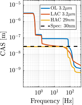

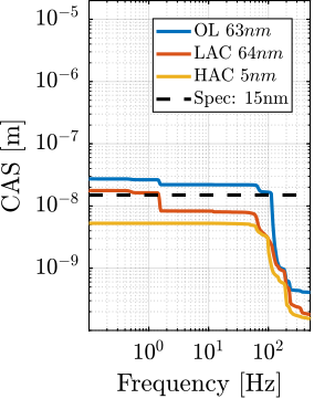
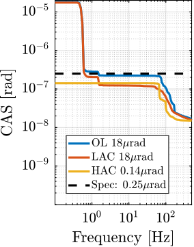
Reflectivity Scans

<<ssec:test_id31_scans_reflectivity>>

X-ray reflectivity measurements involve scanning thin structures, particularly solid/liquid interfaces, through the beam by varying the $R_y$ angle. In this experiment, a $R_y$ scan was executed at a rotational velocity of $100,\mu rad/s$, and the closed-loop positioning errors were monitored (Figure ref:fig:test_id31_reflectivity). The results confirm that the NASS successfully maintains the point of interest within the specified beam parameters throughout the scanning process.

%% Load data for the reflectivity scan
data_ry = load("2023-08-18_15-24_first_reflectivity_m0.mat");
data_ry.time = Ts*[0:length(data_ry.Ry_int)-1];

% Compute closed-loop errors
data_ry.Dy_rms_cl = rms(detrend(data_ry.e_dy,0)); % [m RMS]
data_ry.Dz_rms_cl = rms(detrend(data_ry.e_dz,0)); % [m RMS]
data_ry.Ry_rms_cl = rms(detrend(data_ry.e_ry,0)); % [rad RMS]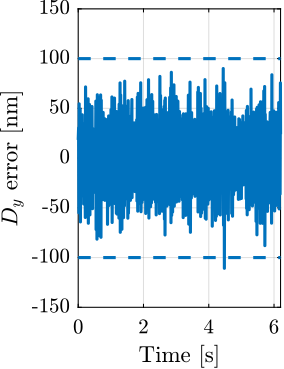

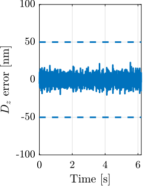
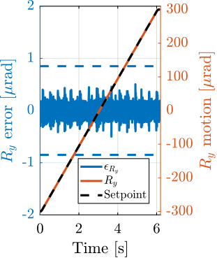
Dirty Layer Scans

<<ssec:test_id31_scans_dz>>

Introduction   ignore

In some cases, samples are composed of several atomic "layers" that are first aligned in the horizontal plane through $R_x$ and $R_y$ positioning, followed by vertical scanning with precise $D_z$ motion. These vertical scans can be executed either continuously or in a step-by-step manner.

Step by Step $D_z$ motion

The vertical step motion is performed exclusively with the nano-hexapod. Testing was conducted across step sizes ranging from $10,nm$ to $1,\mu m$, with results presented in Figure ref:fig:test_id31_dz_mim_steps. The system successfully resolves 10nm steps when detectors integrate over a 50ms period (illustrated by the red curve in Figure ref:fig:test_id31_dz_mim_10nm_steps), which is compatible with many experimental requirements.

In step-by-step scanning procedures, settling time is a critical parameter as it significantly impacts the total experiment duration. The system achieves a response time of approximately $70,ms$ to reach the target position (within $\pm 20,nm$), as demonstrated by the $1,\mu m$ step response in Figure ref:fig:test_id31_dz_mim_1000nm_steps. This settling duration typically decreases for smaller step sizes.

%% Load Dz steps data
data_dz_steps_10nm = load("2023-08-18_14-57_dz_mim_10_nm.mat");
data_dz_steps_10nm.time = Ts*[0:length(data_dz_steps_10nm.Dz_int)-1];

data_dz_steps_100nm = load("2023-08-18_14-57_dz_mim_100_nm.mat");
data_dz_steps_100nm.time = Ts*[0:length(data_dz_steps_100nm.Dz_int)-1];

data_dz_steps_1000nm = load("2023-08-18_14-57_dz_mim_1000_nm.mat");
data_dz_steps_1000nm.time = Ts*[0:length(data_dz_steps_1000nm.Dz_int)-1];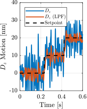

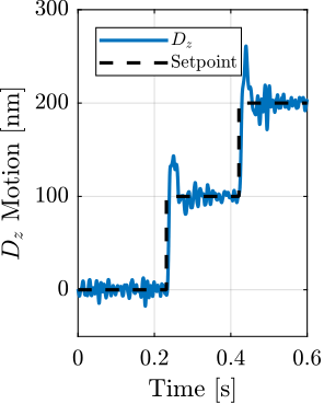
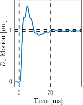
Continuous $D_z$ motion: Dirty Layer Scans

For these and subsequent experiments, the NASS performs "ramp scans" (constant velocity scans). To eliminate tracking errors, the feedback controller incorporates two integrators, compensating for the plant's lack of integral action at low frequencies.

Initial testing at $10,\mu m/s$ demonstrates positioning errors well within specifications (indicated by dashed lines in Figure ref:fig:test_id31_dz_scan_10ums).

%% Dirty layer scans - 10um/s
data_dz_10ums = load("2023-08-18_15-33_dirty_layer_m0_small.mat");
data_dz_10ums.time = Ts*[0:length(data_dz_10ums.Dz_int)-1];

%% Dirty layer scans - 100um/s
data_dz_100ums = load("2023-08-18_15-32_dirty_layer_m0.mat");
data_dz_100ums.time = Ts*[0:length(data_dz_100ums.Dz_int)-1];

%% Performances for Dz scans - 10 um/s
% Determine when the motion starts and stops
i_dz_10ums  = abs(diff(data_dz_10ums.m_hexa_dz)/Ts-10e-6) < 10*eps;

% RMS error
data_dz_10ums.Dy_rms_cl = rms(detrend(data_dz_10ums.e_dy(i_dz_10ums), 0));
data_dz_10ums.Dz_rms_cl = rms(detrend(data_dz_10ums.e_dz(i_dz_10ums), 0));
data_dz_10ums.Ry_rms_cl = rms(detrend(data_dz_10ums.e_ry(i_dz_10ums), 0));

%% Performances for Dz scans - 100 um/s
i_dz_100ums = abs(diff(data_dz_100ums.m_hexa_dz)/Ts-100e-6) < 10*eps;

% RMS error
data_dz_100ums.Dy_rms_cl = rms(detrend(data_dz_100ums.e_dy(i_dz_100ums), 0));
data_dz_100ums.Dz_rms_cl = rms(detrend(data_dz_100ums.e_dz(i_dz_100ums), 0));
data_dz_100ums.Ry_rms_cl = rms(detrend(data_dz_100ums.e_ry(i_dz_100ums), 0));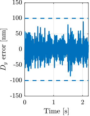

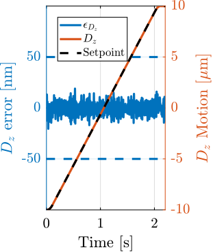
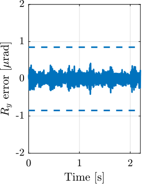
A subsequent scan at $100,\mu m/s$ - the maximum velocity for high-precision $D_z$ scans⁷ - maintains positioning errors within specifications during the constant velocity phase, with deviations occurring only during acceleration and deceleration phases (Figure ref:fig:test_id31_dz_scan_100ums). Since detectors typically operate only during the constant velocity phase, these transient deviations do not compromise measurement quality. Yet, performance during acceleration phases could potentially be enhanced through the implementation of feedforward control.

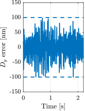
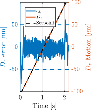
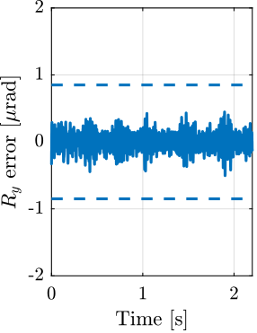
Lateral Scans

<<ssec:test_id31_scans_dy>>

Introduction   ignore

Lateral scans are executed using the $T_y$ stage. The stepper motor controller⁸ generates a setpoint that is transmitted to the Speedgoat. Within the Speedgoat, the system computes the positioning error by comparing the measured $D_y$ sample position against the received setpoint, and the Nano-Hexapod compensates for positioning errors introduced during $T_y$ stage scanning. The scanning range is constrained $\pm 100\,\mu m$ due to the limited acceptance of the metrology system.

Slow scan

Initial testing utilized a scanning velocity of $10,\mu m/s$, which is typical for these experiments. Figure ref:fig:test_id31_dy_10ums compares the positioning errors between open-loop (without NASS) and closed-loop operation. In the scanning direction, open-loop measurements reveal periodic errors (Figure ref:fig:test_id31_dy_10ums_dy) attributable to the $T_y$ stage's stepper motor. These micro-stepping errors, inherent to stepper motor operation, occur 200 times per motor rotation with approximately $1\,\text{mrad}$ angular error amplitude. Given the $T_y$ stage's lead screw pitch of $2\,mm$, these errors manifest as $10\,\mu m$ periodic oscillations with $\approx 300\,nm$ amplitude, which can indeed be seen in the open-loop measurements (Figure ref:fig:test_id31_dy_10ums_dy).

In the vertical direction (Figure ref:fig:test_id31_dy_10ums_dz), open-loop errors likely stem from metrology measurement error due to the fact that the top interferometer points at a spherical target surface (see Figure ref:fig:test_id31_xy_map_sphere). Under closed-loop control, positioning errors remain within specifications across all directions.

%% Slow Ty scan (10um/s) - OL
data_ty_ol_10ums = load("2023-08-21_20-05_ty_scan_m1_open_loop_slow.mat");
data_ty_ol_10ums.time = Ts*[0:length(data_ty_ol_10ums.Dy_int)-1];

%% Slow Ty scan (10um/s) - CL
data_ty_cl_10ums = load("2023-08-21_20-07_ty_scan_m1_cf_closed_loop_slow.mat");
data_ty_cl_10ums.time = Ts*[0:length(data_ty_cl_10ums.Dy_int)-1];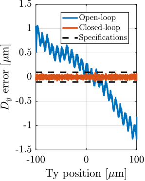

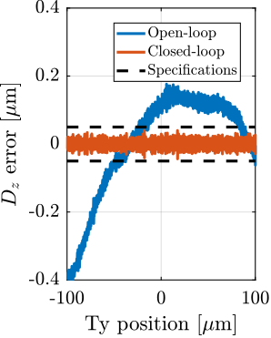
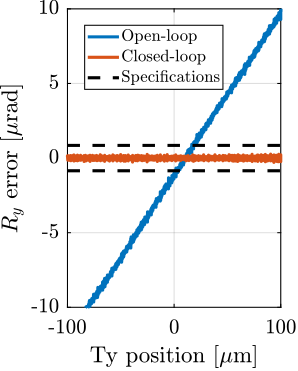
Fast Scan

System performance was evaluated at an increased scanning velocity of $100\,\mu m/s$, with results presented in Figure ref:fig:test_id31_dy_100ums. At this velocity, the micro-stepping errors generate $10\,\text{Hz}$ vibrations, which are further amplified by micro-station resonances. These vibrations exceed the NASS feedback controller bandwidth, resulting in limited attenuation under closed-loop control. This limitation exemplifies why stepper motors are suboptimal for "long-stroke/short-stroke" systems requiring precise scanning performance cite:&dehaeze22_fastj_uhv.

Two potential solutions exist for improving high-velocity scanning performance. First, the $T_y$ stage's stepper motor could be replaced with a three-phase torque motor. Alternatively, since closed-loop errors in $D_z$ and $R_y$ directions remain within specifications (Figures ref:fig:test_id31_dy_100ums_dz and ref:fig:test_id31_dy_100ums_ry), detector triggering could be based on measured $D_y$ position rather than time or $T_y$ setpoint, reducing sensitivity to $D_y$ vibrations. For applications requiring small $D_y$ scans, the nano-hexapod can be used exclusively, though with limited stroke capability.

%% Fast Ty scan (100um/s) - OL
data_ty_ol_100ums = load("2023-08-21_20-05_ty_scan_m1_open_loop.mat");
data_ty_ol_100ums.time = Ts*[0:length(data_ty_ol_100ums.Dy_int)-1];

%% Fast Ty scan (100um/s) - CL
data_ty_cl_100ums = load("2023-08-21_20-07_ty_scan_m1_cf_closed_loop.mat");
data_ty_cl_100ums.time = Ts*[0:length(data_ty_cl_100ums.Dy_int)-1];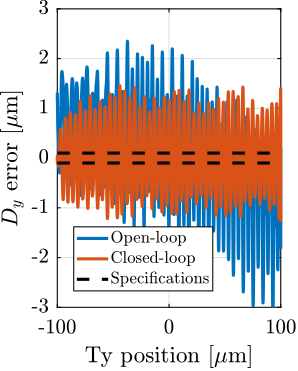

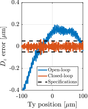
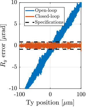
%% Compute errors for Dy scans
i_ty_ol_10ums = data_ty_ol_10ums.Ty > data_ty_ol_10ums.Ty(1) & data_ty_ol_10ums.Ty < data_ty_ol_10ums.Ty(end);
i_ty_cl_10ums = data_ty_cl_10ums.Ty > data_ty_cl_10ums.Ty(1) & data_ty_cl_10ums.Ty < data_ty_cl_10ums.Ty(end);
i_ty_ol_100ums = data_ty_ol_100ums.Ty > data_ty_ol_100ums.Ty(1) & data_ty_ol_100ums.Ty < data_ty_ol_100ums.Ty(end);
i_ty_cl_100ums = data_ty_cl_100ums.Ty > data_ty_cl_100ums.Ty(1) & data_ty_cl_100ums.Ty < data_ty_cl_100ums.Ty(end);

% RMS error
data_ty_ol_10ums.Dy_rms = rms(detrend(data_ty_ol_10ums.e_dy(i_ty_ol_10ums), 0));
data_ty_ol_10ums.Dz_rms = rms(detrend(data_ty_ol_10ums.e_dz(i_ty_ol_10ums), 0));
data_ty_ol_10ums.Ry_rms = rms(detrend(data_ty_ol_10ums.e_ry(i_ty_ol_10ums), 0));

data_ty_cl_10ums.Dy_rms = rms(detrend(data_ty_cl_10ums.e_dy(i_ty_cl_10ums), 0));
data_ty_cl_10ums.Dz_rms = rms(detrend(data_ty_cl_10ums.e_dz(i_ty_cl_10ums), 0));
data_ty_cl_10ums.Ry_rms = rms(detrend(data_ty_cl_10ums.e_ry(i_ty_cl_10ums), 0));

data_ty_ol_100ums.Dy_rms = rms(detrend(data_ty_ol_100ums.e_dy(i_ty_ol_100ums), 0));
data_ty_ol_100ums.Dz_rms = rms(detrend(data_ty_ol_100ums.e_dz(i_ty_ol_100ums), 0));
data_ty_ol_100ums.Ry_rms = rms(detrend(data_ty_ol_100ums.e_ry(i_ty_ol_100ums), 0));

data_ty_cl_100ums.Dy_rms = rms(detrend(data_ty_cl_100ums.e_dy(i_ty_cl_100ums), 0));
data_ty_cl_100ums.Dz_rms = rms(detrend(data_ty_cl_100ums.e_dz(i_ty_cl_100ums), 0));
data_ty_cl_100ums.Ry_rms = rms(detrend(data_ty_cl_100ums.e_ry(i_ty_cl_100ums), 0));

Diffraction Tomography

<<ssec:test_id31_scans_diffraction_tomo>> In diffraction tomography experiments, the micro-station executes combined motions: continuous rotation around the $R_z$ axis while performing lateral scans along $D_y$. For this validation, the spindle maintained a constant rotational velocity of $6\,\text{deg/s}$ while the nano-hexapod executed the lateral scanning motion. To avoid high-frequency vibrations typically induced by the stepper motor, the $T_y$ stage was not utilized, which constrained the scanning range to approximately $\pm 100\,\mu m/s$. The system's performance was evaluated at three lateral scanning velocities: $0.1\,mm/s$, $0.5\,mm/s$, and $1\,mm/s$. Figure ref:fig:test_id31_diffraction_tomo_setpoint presents both the $D_y$ position setpoints and the corresponding measured $D_y$ positions for all tested velocities.

%% 100um/s - Robust controller
data_dt_100ums = load("2023-08-18_17-12_diffraction_tomo_m0.mat");
t = Ts*[0:length(data_dt_100ums.Dy_int)-1];
data_dt_100ums = structfun(@(field) field(t>1.0861),data_dt_100ums, 'UniformOutput', false);
data_dt_100ums.time = Ts*[0:length(data_dt_100ums.Dy_int)-1];

%% 500um/s - Complementary filters
data_dt_500ums = load("2023-08-21_15-15_diffraction_tomo_m0_fast_cf.mat");
t = Ts*[0:length(data_dt_500ums.Dy_int)-1];
data_dt_500ums = structfun(@(field) field(t>0.275),data_dt_500ums, 'UniformOutput', false);
data_dt_500ums.time = Ts*[0:length(data_dt_500ums.Dy_int)-1];

%% 1mm/s - Complementary filters
data_dt_1000ums = load("2023-08-21_15-16_diffraction_tomo_m0_fast_cf.mat");
t = Ts*[0:length(data_dt_1000ums.Dy_int)-1];
data_dt_1000ums = structfun(@(field) field(t>0.19),data_dt_1000ums, 'UniformOutput', false);
data_dt_1000ums.time = Ts*[0:length(data_dt_1000ums.Dy_int)-1];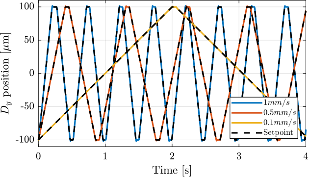

Dy motion for several configured velocities

The positioning errors measured along $D_y$, $D_z$, and $R_y$ directions are displayed in Figure ref:fig:test_id31_diffraction_tomo. The system maintained positioning errors within specifications for both $D_z$ and $R_y$ (Figures ref:fig:test_id31_diffraction_tomo_dz and ref:fig:test_id31_diffraction_tomo_ry). However, lateral positioning errors exceeded specifications during acceleration and deceleration phases (Figure ref:fig:test_id31_diffraction_tomo_dy). Since these large errors occurred only during $\approx 20\,ms$ intervals, the issue could be addressed by implementing a corresponding delay in detector integration. Alternatively, developing a feedforward controller could improve lateral positioning accuracy during these transient phases.

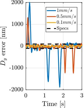
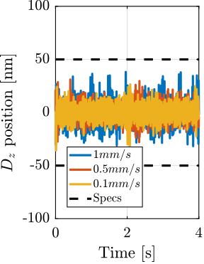
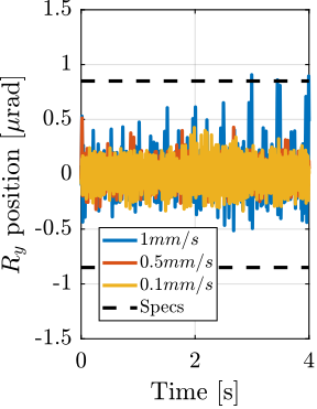
%% Computation of errors during diffraction tomography experiments
% Ignore acceleration and deceleration phases
acc_dt = 20e-3; % Acceleration phase to remove [s]
acc_n = acc_dt/Ts; % Number of points to delete

% Determine when the motion starts and stops
i_dt_100ums  = data_dt_100ums.m_hexa_dy>data_dt_100ums.m_hexa_dy(1) & data_dt_100ums.m_hexa_dy<data_dt_100ums.m_hexa_dy(end);
[~, i_acc] = find(diff(i_dt_100ums)>0); % Acceleration phases
for i = i_acc
    i_dt_100ums(i:i+acc_n) = 0;
end
[~, i_dec] = find(diff(i_dt_100ums)<0); % Deceleration phases
for i = i_dec(2:2:end)
    i_dt_100ums(i-acc_n:i) = 0;
end

i_dt_500ums  = data_dt_500ums.m_hexa_dy>data_dt_500ums.m_hexa_dy(1) & data_dt_500ums.m_hexa_dy<data_dt_500ums.m_hexa_dy(end);
[~, i_acc] = find(diff(i_dt_500ums)>0); % Acceleration phases
for i = i_acc
    i_dt_500ums(i:i+acc_n) = 0;
end
[~, i_dec] = find(diff(i_dt_500ums)<0); % Deceleration phases
for i = i_dec(2:2:end)
    i_dt_500ums(i-acc_n:i) = 0;
end

i_dt_1000ums  = data_dt_1000ums.m_hexa_dy>data_dt_1000ums.m_hexa_dy(1) & data_dt_1000ums.m_hexa_dy<data_dt_1000ums.m_hexa_dy(end);
[~, i_acc] = find(diff(i_dt_1000ums)>0); % Acceleration phases
for i = i_acc
    i_dt_1000ums(i:i+acc_n) = 0;
end
[~, i_dec] = find(diff(i_dt_1000ums)<0); % Deceleration phases
for i = i_dec(2:2:end)
    i_dt_1000ums(i-acc_n:i) = 0;
end

% RMS error
data_dt_100ums.Dy_rms_cl = rms(detrend(data_dt_100ums.Dy_int(i_dt_100ums)-data_dt_100ums.m_hexa_dy(i_dt_100ums), 0));
data_dt_100ums.Dz_rms_cl = rms(detrend(data_dt_100ums.Dz_int(i_dt_100ums), 0));
data_dt_100ums.Ry_rms_cl = rms(detrend(data_dt_100ums.Ry_int(i_dt_100ums), 0));

data_dt_500ums.Dy_rms_cl = rms(detrend(data_dt_500ums.Dy_int(i_dt_500ums)-data_dt_500ums.m_hexa_dy(i_dt_500ums), 0));
data_dt_500ums.Dz_rms_cl = rms(detrend(data_dt_500ums.Dz_int(i_dt_500ums), 0));
data_dt_500ums.Ry_rms_cl = rms(detrend(data_dt_500ums.Ry_int(i_dt_500ums), 0));

data_dt_1000ums.Dy_rms_cl = rms(detrend(data_dt_1000ums.Dy_int(i_dt_1000ums)-data_dt_1000ums.m_hexa_dy(i_dt_1000ums), 0));
data_dt_1000ums.Dz_rms_cl = rms(detrend(data_dt_1000ums.Dz_int(i_dt_1000ums), 0));
data_dt_1000ums.Ry_rms_cl = rms(detrend(data_dt_1000ums.Ry_int(i_dt_1000ums), 0));

Conclusion

<<ssec:test_id31_scans_conclusion>>

A comprehensive series of experimental validations was conducted to evaluate the NASS performance across a wide range of typical scientific experiments. The system demonstrated robust performance in most scenarios, with positioning errors generally remaining within specified tolerances (30 nm RMS in $D_y$, 15 nm RMS in $D_z$, and 250 nrad RMS in $R_y$).

For tomography experiments, the NASS successfully maintained positioning accuracy at rotational velocities up to $180\,\text{deg/s}$ with light payloads, though performance degraded somewhat with heavier masses. The HAC-LAC control architecture proved particularly effective, with the decentralized IFF providing damping of nano-hexapod suspension modes while the high authority controller addressed low-frequency disturbances.

Vertical scanning capabilities were validated in both step-by-step and continuous motion modes. The system successfully resolved 10 nm steps with 50 ms detector integration time, while maintaining positioning accuracy during continuous scans at speeds up to $100\,\mu m/s$.

For lateral scanning, the system performed well at moderate speeds ($10\,\mu m/s$) but showed limitations at higher velocities ($100\,\mu m/s$) due to stepper motor-induced vibrations in the $T_y$ stage.

The most challenging test case - diffraction tomography combining rotation and lateral scanning - demonstrated the system's ability to maintain vertical and angular stability while highlighting some limitations in lateral positioning during rapid accelerations. These limitations could potentially be addressed through feedforward control or alternative detector triggering strategies.

Overall, the experimental results validate the effectiveness of the developed control architecture and demonstrate that the NASS meets most design specifications across a wide range of operating conditions (summarized in Table ref:tab:test_id31_experiments_results_summary). The identified limitations, primarily related to high-speed lateral scanning and heavy payload handling, provide clear directions for future improvements.

%% Summary of results
% 1e9*data_tomo_m0_Wz6.Dy_rms_ol,   1e9*data_tomo_m0_Wz6.Dz_rms_ol,   1e6*data_tomo_m0_Wz6.Ry_rms_ol; %   Tomo - OL - 6deg/s - 0kg
% 1e9*data_tomo_m0_Wz6.Dy_rms_cl,   1e9*data_tomo_m0_Wz6.Dz_rms_cl,   1e6*data_tomo_m0_Wz6.Ry_rms_cl; %   Tomo - CL - 6deg/s - 0kg
% 1e9*data_tomo_m1_Wz6.Dy_rms_ol,   1e9*data_tomo_m1_Wz6.Dz_rms_ol,   1e6*data_tomo_m1_Wz6.Ry_rms_ol; %   Tomo - OL - 6deg/s - 13kg
% 1e9*data_tomo_m1_Wz6.Dy_rms_cl,   1e9*data_tomo_m1_Wz6.Dz_rms_cl,   1e6*data_tomo_m1_Wz6.Ry_rms_cl; %   Tomo - CL - 6deg/s - 13kg
% 1e9*data_tomo_m2_Wz6.Dy_rms_ol,   1e9*data_tomo_m2_Wz6.Dz_rms_ol,   1e6*data_tomo_m2_Wz6.Ry_rms_ol; %   Tomo - OL - 6deg/s - 26kg
% 1e9*data_tomo_m2_Wz6.Dy_rms_cl,   1e9*data_tomo_m2_Wz6.Dz_rms_cl,   1e6*data_tomo_m2_Wz6.Ry_rms_cl; %   Tomo - CL - 6deg/s - 26kg
% 1e9*data_tomo_m3_Wz6.Dy_rms_ol,   1e9*data_tomo_m3_Wz6.Dz_rms_ol,   1e6*data_tomo_m3_Wz6.Ry_rms_ol; %   Tomo - OL - 6deg/s - 39kg
% 1e9*data_tomo_m3_Wz6.Dy_rms_cl,   1e9*data_tomo_m3_Wz6.Dz_rms_cl,   1e6*data_tomo_m3_Wz6.Ry_rms_cl; %   Tomo - CL - 6deg/s - 39kg
% 1e9*data_tomo_m0_Wz180.Dy_rms_ol, 1e9*data_tomo_m0_Wz180.Dz_rms_ol, 1e6*data_tomo_m0_Wz180.Ry_rms_ol; % Tomo - OL - 180deg/s - 0kg
% 1e9*data_tomo_m0_Wz180.Dy_rms_cl, 1e9*data_tomo_m0_Wz180.Dz_rms_cl, 1e6*data_tomo_m0_Wz180.Ry_rms_cl; % Tomo - CL - 180deg/s - 0kg
% 1e9*data_hac_Wz180.Dy_rms_cl,     1e9*data_hac_Wz180.Dz_rms_cl,     1e6*data_hac_Wz180.Ry_rms_cl; %     Tomo - CL (high performance HAC) - 180deg/s - 0kg
% 1e9*data_ry.Dy_rms_cl,            1e9*data_ry.Dz_rms_cl,            1e6*data_ry.Ry_rms_cl; %            Ry 100urad/s
% 1e9*data_dz_10ums.Dy_rms_cl,      1e9*data_dz_10ums.Dz_rms_cl,      1e6*data_dz_10ums.Ry_rms_cl; %      Dz 10um/s
% 1e9*data_dz_100ums.Dy_rms_cl,     1e9*data_dz_100ums.Dz_rms_cl,     1e6*data_dz_100ums.Ry_rms_cl; %     Dz 100um/s
% 1e9*data_ty_ol_10ums.Dy_rms,      1e9*data_ty_ol_10ums.Dz_rms,      1e6*data_ty_ol_10ums.Ry_rms; %      Ty - OL - 10um/s
% 1e9*data_ty_cl_10ums.Dy_rms,      1e9*data_ty_cl_10ums.Dz_rms,      1e6*data_ty_cl_10ums.Ry_rms; %      Ty - CL - 10um/s
% 1e9*data_ty_ol_100ums.Dy_rms,     1e9*data_ty_ol_100ums.Dz_rms,     1e6*data_ty_ol_100ums.Ry_rms; %     Ty - OL - 100um/s
% 1e9*data_ty_cl_100ums.Dy_rms,     1e9*data_ty_cl_100ums.Dz_rms,     1e6*data_ty_cl_100ums.Ry_rms; %     Ty - CL - 100um/s
% 1e9*data_dt_100ums.Dy_rms_cl,     1e9*data_dt_100ums.Dz_rms_cl,     1e6*data_dt_100ums.Ry_rms_cl; %     Diffraction Tomo - CL - 6deg/s,  100um/s
% 1e9*data_dt_500ums.Dy_rms_cl,     1e9*data_dt_500ums.Dz_rms_cl,     1e6*data_dt_500ums.Ry_rms_cl; %     Diffraction Tomo - CL - 6deg/s,  500um/s
% 1e9*data_dt_1000ums.Dy_rms_cl,    1e9*data_dt_1000ums.Dz_rms_cl,    1e6*data_dt_1000ums.Ry_rms_cl; %    Diffraction Tomo - CL - 6deg/s, 1000um/s

Experiments	$\bm{D_y}$ [nmRMS]	$\bm{D_z}$ [nmRMS]	$\bm{R_y}$ [nradRMS]
Tomography ($6\,\text{deg/s}$)	$142 \Rightarrow 15$	$32 \Rightarrow 5$	$464 \Rightarrow 56$
Tomography ($6\,\text{deg/s}$, 13kg)	$149 \Rightarrow 25$	$26 \Rightarrow 6$	$471 \Rightarrow 55$
Tomography ($6\,\text{deg/s}$, 26kg)	$202 \Rightarrow 25$	$36 \Rightarrow 7$	$1737 \Rightarrow 104$
Tomography ($6\,\text{deg/s}$, 39kg)	$297 \Rightarrow \bm{53}$	$38 \Rightarrow 9$	$1737 \Rightarrow 170$
Tomography ($180\,\text{deg/s}$)	$143 \Rightarrow \bm{38}$	$24 \Rightarrow 11$	$252 \Rightarrow 130$
Tomography ($180\,\text{deg/s}$, custom HAC)	$143 \Rightarrow 29$	$24 \Rightarrow 5$	$252 \Rightarrow 142$
Reflectivity ($100\,\mu\text{rad}/s$)	$28$	$6$	$118$
$D_z$ scan ($10\,\mu m/s$)	$25$	$5$	$108$
$D_z$ scan ($100\,\mu m/s$)	$\bm{35}$	$9$	$132$
Lateral Scan ($10\,\mu m/s$)	$585 \Rightarrow 21$	$155 \Rightarrow 10$	$6300 \Rightarrow 60$
Lateral Scan ($100\,\mu m/s$)	$1063 \Rightarrow \bm{732}$	$167 \Rightarrow \bm{20}$	$6445 \Rightarrow \bm{356}$
Diffraction tomography ($6\,\text{deg/s}$, $0.1\,mm/s$)	$\bm{36}$	$7$	$113$
Diffraction tomography ($6\,\text{deg/s}$, $0.5\,mm/s$)	$29$	$8$	$81$
Diffraction tomography ($6\,\text{deg/s}$, $1\,mm/s$)	$\bm{53}$	$10$	$135$
Specifications	$30$	$15$	$250$

Conclusion

<<ssec:test_id31_conclusion>>

This chapter presented a comprehensive experimental validation of the Nano Active Stabilization System (NASS) on the ID31 beamline, demonstrating its capability to maintain precise sample positioning during various experimental scenarios. The implementation and testing followed a systematic approach, beginning with the development of a short-stroke metrology system to measure the sample's position, followed by the successful implementation of a HAC-LAC control architecture, and concluding in extensive performance validation across diverse experimental conditions.

The short-stroke metrology system, while designed as an temporary solution, proved effective in providing high bandwidth and low noise 5-DoF position measurements. The careful alignment of the fibered interferometers targeting two reference spheres ensured reliable measurements throughout the testing campaign.

The implementation of the control architecture validated the theoretical framework developed earlier in the project. The decentralized Integral Force Feedback (IFF) controller successfully provided robust damping of suspension modes across all payload conditions (0-39 kg), reducing peak amplitudes by approximately a factor of 10. The High Authority Controller (HAC) effectively managed low-frequency disturbances, though its performance showed some dependency on payload mass, particularly for lateral motion control.

The experimental validation encompassed a wide range of scientific scenarios. The system demonstrated remarkable performance in most conditions, meeting the stringent positioning requirements (30 nm RMS in $D_y$, 15 nm RMS in $D_z$, and 250 nrad RMS in $R_y$) for the majority of test cases. Some limitations were identified, particularly in handling heavy payloads during rapid motions and in managing high-speed lateral scanning with the existing stepper motor $T_y$ stage.

The successful validation of the NASS demonstrates that, once an accurate online metrology system is developed, it will be ready for integration into actual beamline operations. The system's ability to maintain precise sample positioning across a wide range of experimental conditions, combined with its robust performance and adaptive capabilities, suggests it will significantly enhance the quality and efficiency of X-ray experiments at ID31. Moreover, the systematic approach to system development and validation, along with the detailed understanding of performance limitations, provides valuable insights for future improvements and potential applications in similar high-precision positioning systems.

Bibliography   ignore

Footnotes

⁷Such scan could corresponding to a 1ms integration time (which is typically the smallest integration time) and 100nm "resolution" (equal to the vertical beam size). ⁶The highest rotational velocity of $360\,\text{deg/s}$ could not be tested due to an issue in the Spindle's controller. ³The roundness of the spheres is specified at $50\,nm$. ⁸The "IcePAP" cite:&janvier13_icepap which is developed at the ESRF. ⁵Note that the eccentricity of the "point of interest" with respect to the Spindle rotation axis has been tuned based on measurements. ⁴The "PEPU" cite:&hino18_posit_encod_proces_unit was used for digital protocol conversion between the interferometers and the Speedgoat. ²M12/F40 model from Attocube. ¹Depending on the measuring range, gap can range from $\approx 1\,\mu m$ to $\approx 100\,\mu m$.

---