phd-test-bench-flexible-joints/test-bench-flexible-joints.org

Flexible Joints - Test Bench

• Introduction
• Dimensional Measurements
  • Measurement Bench
  • Measurement Results
  • Bad flexible joints
• Development of the Measurement Test Bench
  • Introduction
  • Measurement principle
    • Required external applied force
    • Required actuator stroke and sensors range
  • Developped test bench
  • Error budget
    • Introduction
    • Finite Element Model
    • Setup
    • Effect of Bending
    • Computation of the bending stiffness
    • Estimation error due to force and displacement sensors accuracy
    • Estimation error due to Shear
    • Estimation error due to force sensor compression
    • Estimation error due to height estimation error
    • Conclusion
• Bending Stiffness Measurement
  • Introduction
  • Force Sensor Calibration
  • Force Sensor Stiffness
  • Analysis of one measurement
  • Bending stiffness and bending stroke of all the flexible joints
  • Analysis
  • Conclusion
• Conclusion
• Bibliography
• Footnotes

---

This report is also available as a pdf.

---

Introduction   ignore

At both ends of the nano-hexapod struts, a flexible spherical joint is used. Ideally, these flexible joints would behave as perfect spherical joints, that is to say no bending and torsional stiffnesses, infinite shear and axial stiffnesses, unlimited bending and torsional stroke, no friction and no backlash.

Deviations from this ideal properties will impact the dynamics of the Nano-Hexapod and could limit the attainable performances. During the detailed design phase, specifications in term of stiffness and stroke have been determined and are summarized in Table ref:tab:test_joints_specs.

	Specification	FEM
Axial Stiffness	$> 100\,N/\mu m$	94
Shear Stiffness	$> 1\,N/\mu m$	13
Bending Stiffness	$< 100\,Nm/\text{rad}$	5
Torsion Stiffness	$< 500\,Nm/\text{rad}$	260
Bending Stroke	$> 1\,\text{mrad}$	24.5
Torsion Stroke	$> 5\,\mu\text{rad}$

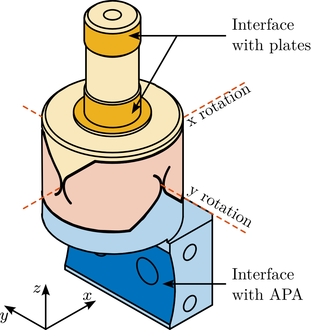
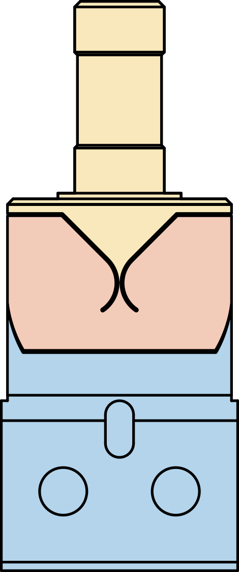
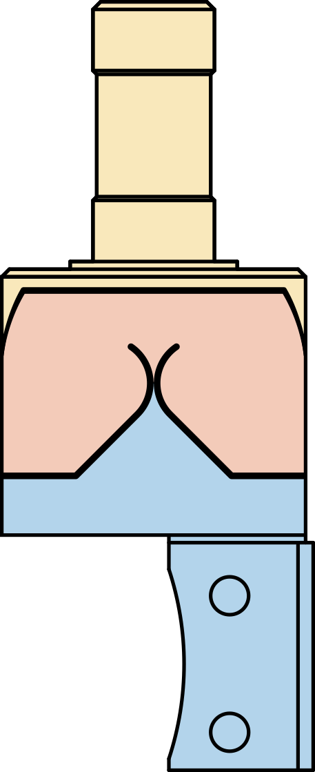
After optimization using a finite element model, the geometry shown in Figure ref:fig:test_joints_schematic has been obtained and the corresponding flexible joints characteristics are summarized in Table ref:tab:test_joints_specs. This flexible joint is a monolithic piece of stainless steel¹ manufactured using wire electrical discharge machining. It serves several functions as shown in Figure ref:fig:test_joints_iso, such as:

• Rigid interfacing with the nano-hexapod plates (yellow surfaces)
• Rigid interfacing with the amplified piezoelectric actuator (blue surface)
• Allow two rotations between the "yellow" and the "blue" interfaces. The rotation axes are represented by the dashed lines which are intersecting

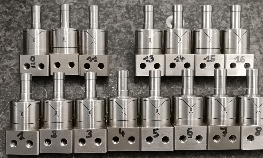
16 flexible joints have been ordered (shown in Figure ref:fig:test_joints_received) such some selection can be made for the 12 that will be used on the nano-hexapod.

In this document, the received flexible joints are characterize to make sure they are fulfilling the requirements and such that they can well be modelled.

First, the flexible joints are visually inspected, and the minimum gaps (responsible for most of the joint compliance) are measured (Section ref:sec:test_joints_flex_dim_meas). Then, a test bench is developed to measure the bending stiffness of the flexible joints. The development of this test bench is presented in Section ref:sec:test_joints_test_bench_desc, including a noise budget and some requirements in terms of instrumentation. Finally, the test bench is manufacturer and used to measure the bending stiffnesses of all the flexible joints. Results are shown in Section ref:sec:test_joints_bending_stiffness_meas

Sections	Matlab File
Section ref:sec:test_joints_flex_dim_meas	test_joints_1_dim_meas.m
Section ref:sec:test_joints_test_bench_desc	test_joints_2_bench_dimensioning.m
Section ref:sec:test_joints_bending_stiffness_meas	test_joints_3_bending_stiff_meas.m

Dimensional Measurements

<<sec:test_joints_flex_dim_meas>>

Measurement Bench

The dimensions of the flexible part in the Y-Z plane will contribute to the X-bending stiffness. Similarly, the dimensions of the flexible part in the X-Z plane will contribute to the Y-bending stiffness.

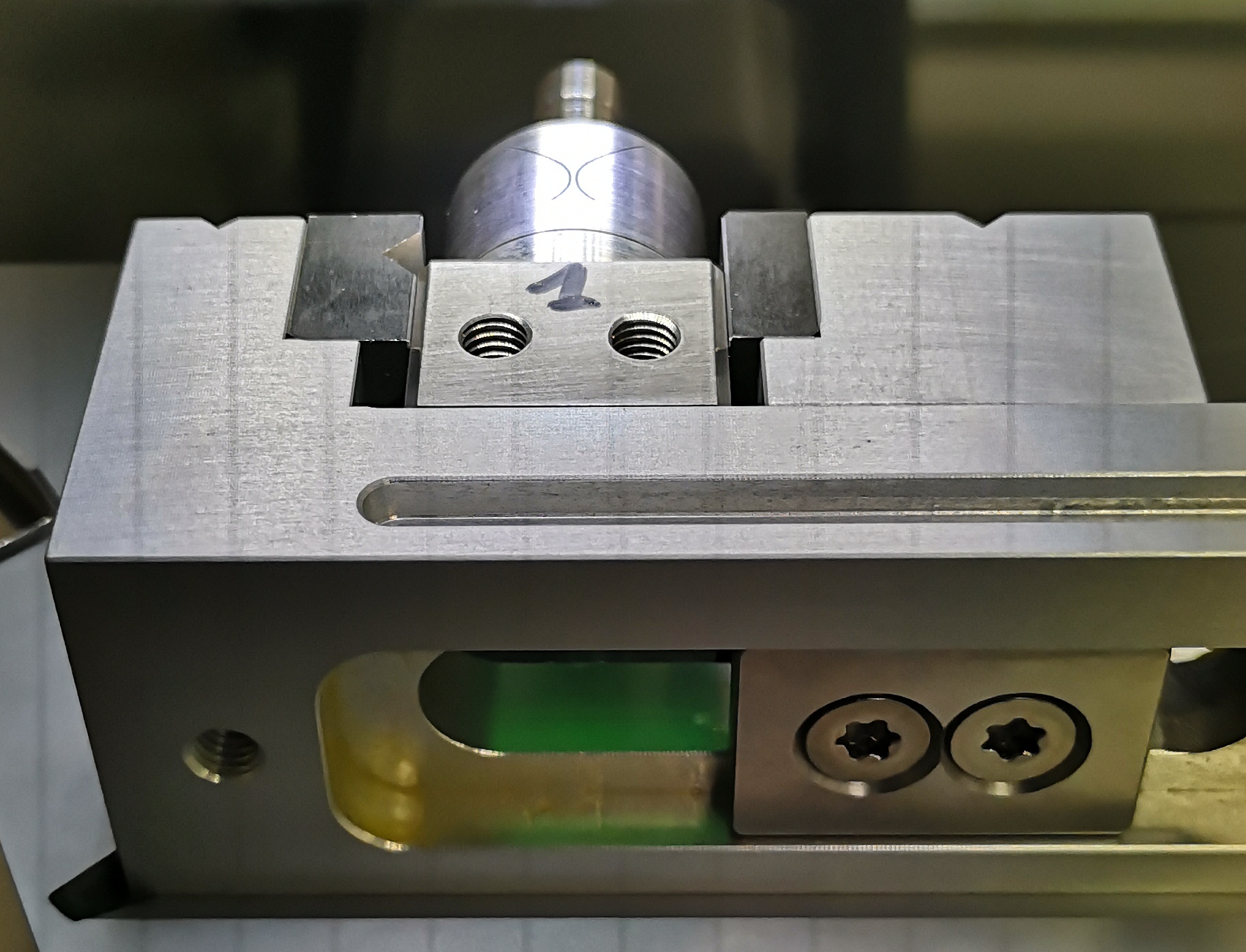
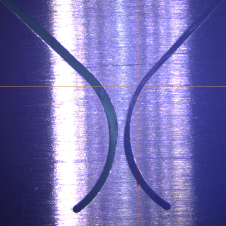
The setup to measure the dimension of the "X" flexible beam is shown in Figure ref:fig:test_joints_profilometer_setup.

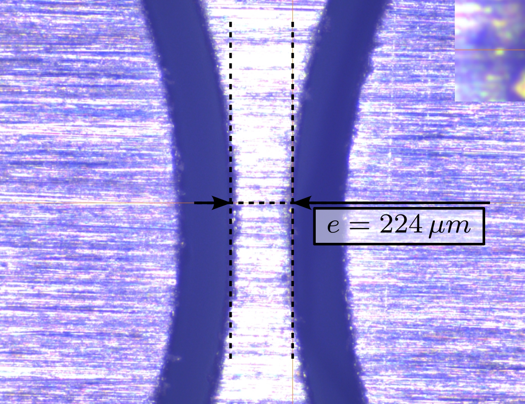
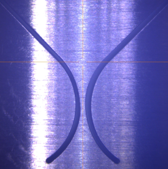
What we typically observe is shown in Figure ref:fig:test_joints_profilometer_image. It is then possible to estimate to dimension of the flexible beam with an accuracy of $\approx 5\,\mu m$,

Measurement Results

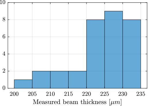
The specified flexible beam thickness (gap) is $250\,\mu m$. Four gaps are measured for each flexible joints (2 in the $x$ direction and 2 in the $y$ direction). The "beam thickness" is then estimated to be the mean between the gaps measured on opposite sides.

An histogram of the measured beam thicknesses is shown in Figure ref:fig:test_joints_size_hist. The measured thickness is less thant the specified value of $250\,\mu m$, but this optical method may not be very accurate as the estimated gap can depend on the lighting of the part and of its proper alignment.

However, what is more important than the true value of the thickness is the consistency between all the flexible joints.

Histogram for the (16x2) measured beams' thickness

Bad flexible joints

Using this profilometer allowed to detect flexible joints with manufacturing defects such as non-symmetrical shape (see Figure ref:fig:test_joints_bad_shape) or flexible joints with machining chips stuck in the gap (see Figure ref:fig:test_joints_bad_chips).

Development of the Measurement Test Bench

<<sec:test_joints_test_bench_desc>>

Introduction   ignore

The most important characteristic of the flexible joint to be measured is its bending stiffness $k_{R_x} \approx k_{R_y}$.

To estimate the bending stiffness, the basic idea is to apply a torque $T_{x}$ to the flexible joints and to measure its angular deflection $\theta_{x}$. Then, the bending stiffness can be computed from equation eqref:eq:test_joints_bending_stiffness.

\begin{equation}\label{eq:test_joints_bending_stiffness} k_{R_x} = \frac{T_x}{θ_x}

\end{equation}

Measurement principle

As it is difficult to apply a pure torque, a "linear" force can be applied instead. The application point of the force should be far enough from the rotation axis such that the resulting bending motion is much larger than the displacement due to shear.

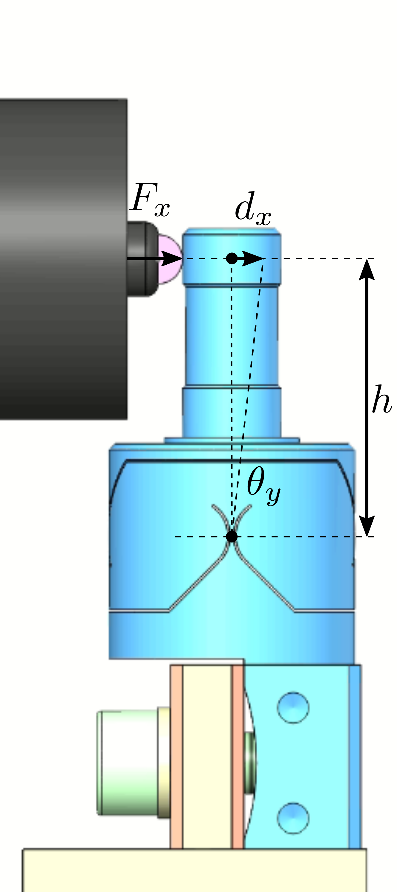
The working principle of the measurement bench is schematically shown in Figure ref:fig:test_joints_bench_working_principle. One part of the flexible joint is fixed. On the mobile part, a force $F_x$ is applied which is equivalent to a torque applied on the flexible joint center. The induced rotation is measured with a displacement sensor $d_x$.

Test Bench - working principle

Geometry of the flexible joint

This test-bench will be used to have a first approximation of the bending stiffnesss and stroke of the flexible joints.

The flexible joint used for the Nano-Hexapod is shown in Figure ref:fig:test_joints_bend_geometry. Its bending stiffness is foreseen to be $k_{R_y}\approx 5\,\frac{Nm}{rad}$ and its stroke $\theta_{y,\text{max}}\approx 25\,mrad$.

The height between the flexible point (center of the joint) and the point where external forces are applied is $h = 20\,mm$.

Let's define the parameters on Matlab.

kRx = 5; % Bending Stiffness [Nm/rad]
Rxmax = 25e-3; % Bending Stroke [rad]
h = 20e-3; % Height [m]

Required external applied force

The bending $\theta_y$ of the flexible joint due to the force $F_x$ is:

\begin{equation} \theta_y = \frac{M_y}{k_{R_y}} = \frac{F_x h}{k_{R_y}} \end{equation}

Therefore, the applied force to test the full range of the flexible joint is:

\begin{equation} F_{x,\text{max}} = \frac{k_{R_y} \theta_{y,\text{max}}}{h} \end{equation}

Fxmax = kRx*Rxmax/h; % Force to induce maximum stroke [N]

And we obtain:

\begin{equation} F_{x,max} = 6.2\, [N] \end{equation}

The measurement range of the force sensor should then be higher than $6.2\,N$.

Required actuator stroke and sensors range

The flexible joint is designed to allow a bending motion of $\pm 25\,mrad$. The corresponding stroke at the location of the force sensor is: \[ d_{x,\text{max}} = h \tan(R_{x,\text{max}}) \]

dxmax = h*tan(Rxmax);

\begin{equation} d_{max} = 0.5\, [mm] \end{equation}

In order to test the full range of the flexible joint, the stroke of the translation stage used to move the force sensor should be higher than $0.5\,mm$. Similarly, the measurement range of the displacement sensor should also be higher than $0.5\,mm$.

Developped test bench

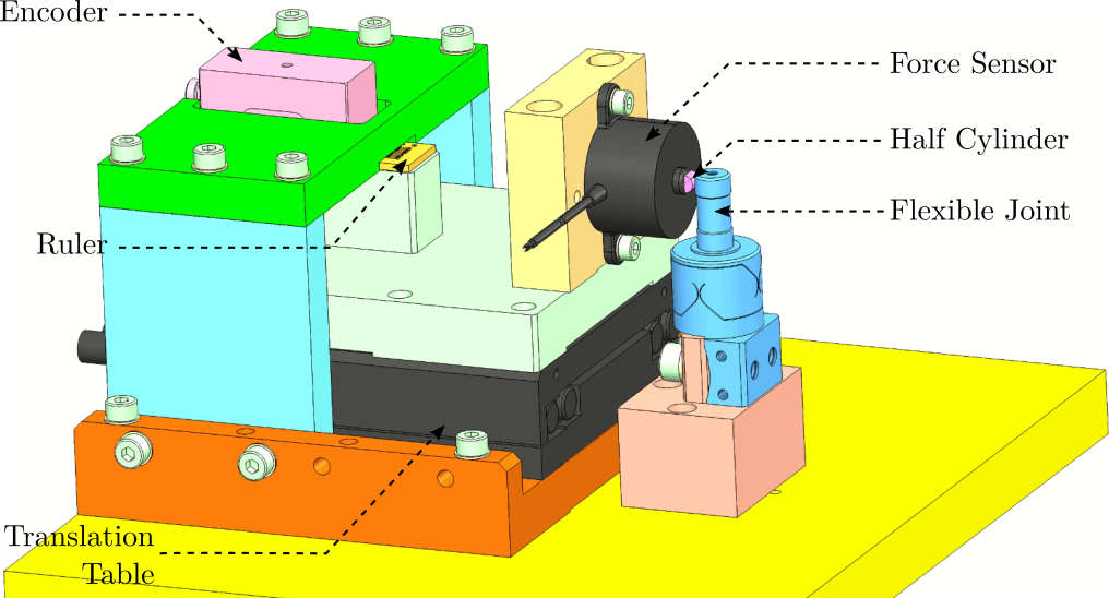
A CAD view of the measurement bench is shown in Figure ref:fig:test_joints_bench_overview.

Here are the different elements used in this bench:

• Translation Stage: V-408
• Load Cells: FC2231-0000-0010-L
• Encoder: Renishaw Resolute 1nm

Both the measured force and displacement are acquired at the same time using a Speedgoat machine. Explain why the encoder is here: in line with the measurement, no "abbe errors"

A side view of the bench with the important quantities are shown in Figure ref:fig:test_joints_bench_side.

Error budget

<<ssec:test_joints_error_budget>>

Introduction   ignore

Many things can impact the accuracy of the measured bending stiffness such as:

• Errors in the force and displacement measurement
• Shear effects
• Deflection of the Force sensor
• Errors in the geometry of the bench

In this section, we wish to estimate the attainable accuracy with the current bench, and identified the limiting factors.

Finite Element Model

From the Finite Element Model, the stiffness and stroke of the flexible joint have been computed and summarized in Tables ref:tab:test_joints_axial_shear_prop and ref:tab:test_joints_bending_torsion_prop.

	Stiffness [N/um]	Max Force [N]	Stroke [um]
Axial	94	469	5
Shear	13	242	19

	Stiffness [Nm/rad]	Max Torque [Nmm]	Stroke [mrad]
Bending	5	118	24
Torsional	260	1508	6

Setup

The setup is schematically represented in Figure ref:fig:test_joints_bench_side_bis.

The force is applied on top of the flexible joint with a distance $h$ with the joint's center. The displacement of the flexible joint is also measured at the same height.

The height between the joint's center and the force application point is:

h = 25e-3; % Height [m]

Effect of Bending

The torque applied is:

\begin{equation} M_y = F_x \cdot h \end{equation}

The flexible joint is experiencing a rotation $\theta_y$ due to the torque $M_y$:

\begin{equation} \theta_y = \frac{M_y}{k_{R_y}} = \frac{F_x \cdot h}{k_{R_y}} \end{equation}

This rotation is then measured by the displacement sensor. The measured displacement is:

\begin{equation} D_b = h \tan(\theta_y) = h \tan\left( \frac{F_x \cdot h}{k_{R_y}} \right) \label{eq:bending_stiffness_formula} \end{equation}

Computation of the bending stiffness

From equation eqref:eq:bending_stiffness_formula, we can compute the bending stiffness:

\begin{equation} k_{R_y} = \frac{F_x \cdot h}{\tan^{-1}\left( \frac{D_b}{h} \right)} \end{equation}

For small displacement, we have

\begin{equation} \boxed{k_{R_y} \approx h^2 \frac{F_x}{d_x}} \end{equation}

And therefore, to precisely measure $k_{R_y}$, we need to:

• precisely measure the motion $d_x$
• precisely measure the applied force $F_x$
• precisely now the height of the force application point $h$

Estimation error due to force and displacement sensors accuracy

The maximum error on the measured displacement with the encoder is 40 nm. This quite negligible compared to the measurement range of 0.5 mm.

The accuracy of the force sensor is around 1% and therefore, we should expect to have an accuracy on the measured stiffness of at most 1%.

Estimation error due to Shear

The effect of Shear on the measured displacement is simply:

\begin{equation} D_s = \frac{F_x}{k_s} \end{equation}

The measured displacement will be the effect of shear + effect of bending

\begin{equation} d_x = D_b + D_s = h \tan\left( \frac{F_x \cdot h}{k_{R_y}} \right) + \frac{F_x}{k_s} \approx F_x \left( \frac{h^2}{k_{R_y}} + \frac{1}{k_s} \right) \end{equation}

The estimated bending stiffness $k_{\text{est}}$ will then be:

\begin{equation} k_{\text{est}} = h^2 \frac{F_x}{d_x} \approx k_{R_y} \frac{1}{1 + \frac{k_{R_y}}{k_s h^2}} \end{equation}

The measurement error due to Shear is 0.1 %

Estimation error due to force sensor compression

The measured displacement is not done directly at the joint's location. The force sensor compression will then induce an error on the joint's stiffness.

The force sensor stiffness $k_F$ is estimated to be around:

kF = 50/0.05e-3; % [N/m]

k_F = 1.0e+06 [N/m]

The measured displacement will be the sum of the displacement induced by the bending and by the compression of the force sensor:

\begin{equation} d_x = D_b + \frac{F_x}{k_F} = h \tan\left( \frac{F_x \cdot h}{k_{R_y}} \right) + \frac{F_x}{k_F} \approx F_x \left( \frac{h^2}{k_{R_y}} + \frac{1}{k_F} \right) \end{equation}

The estimated bending stiffness $k_{\text{est}}$ will then be:

\begin{equation} k_{\text{est}} = h^2 \frac{F_x}{d_x} \approx k_{R_y} \frac{1}{1 + \frac{k_{R_y}}{k_F h^2}} \end{equation}

The measurement error due to height estimation errors is 0.8 %

Estimation error due to height estimation error

Let's consider an error in the estimation of the height from the application of the force to the joint's center:

\begin{equation} h_{\text{est}} = h (1 + \epsilon) \end{equation}

The computed bending stiffness will be:

\begin{equation} k_\text{est} \approx h_{\text{est}}^2 \frac{F_x}{d_x} \end{equation}

And the stiffness estimation error is:

\begin{equation} \frac{k_{\text{est}}}{k_{R_y}} = (1 + \epsilon)^2 \end{equation}

h_err = 0.2e-3; % Height estimation error [m]

The measurement error due to height estimation errors of 0.2 [mm] is 1.6 %

Conclusion

Based on the above analysis, we should expect no better than few percent of accuracy using the current test-bench. This is well enough for a first estimation of the bending stiffness of the flexible joints.

Bending Stiffness Measurement

<<sec:test_joints_bending_stiffness_meas>>

Introduction

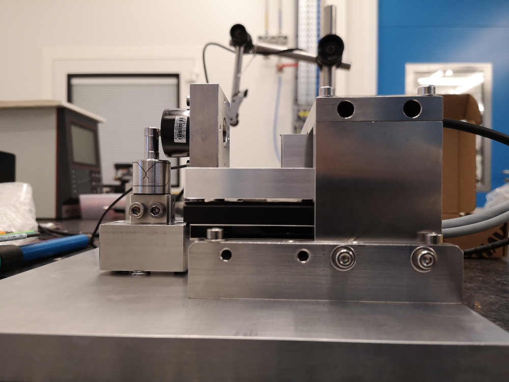
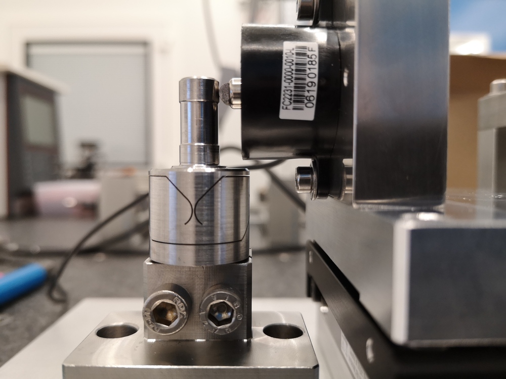
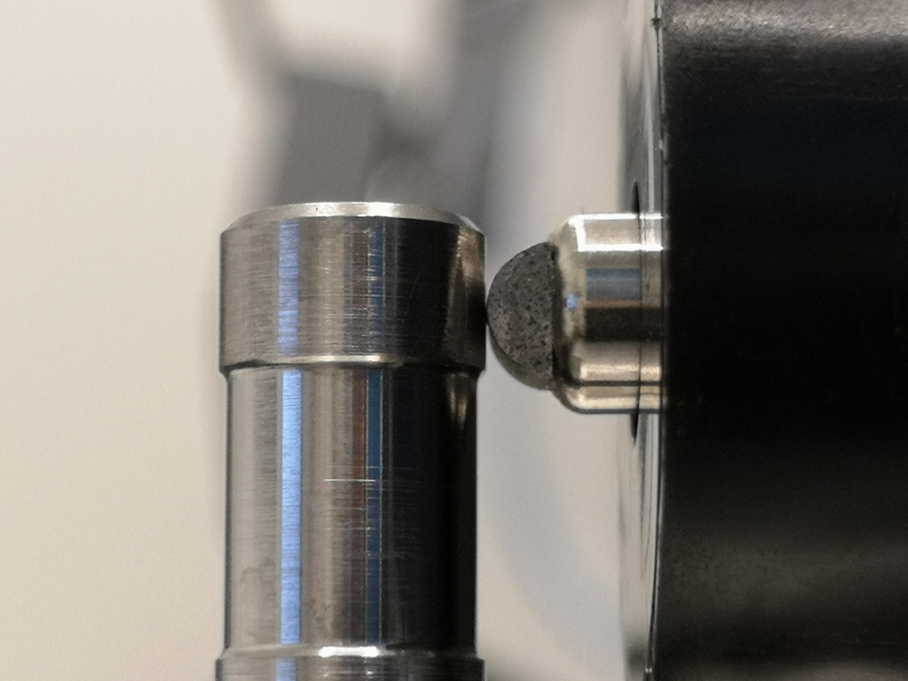
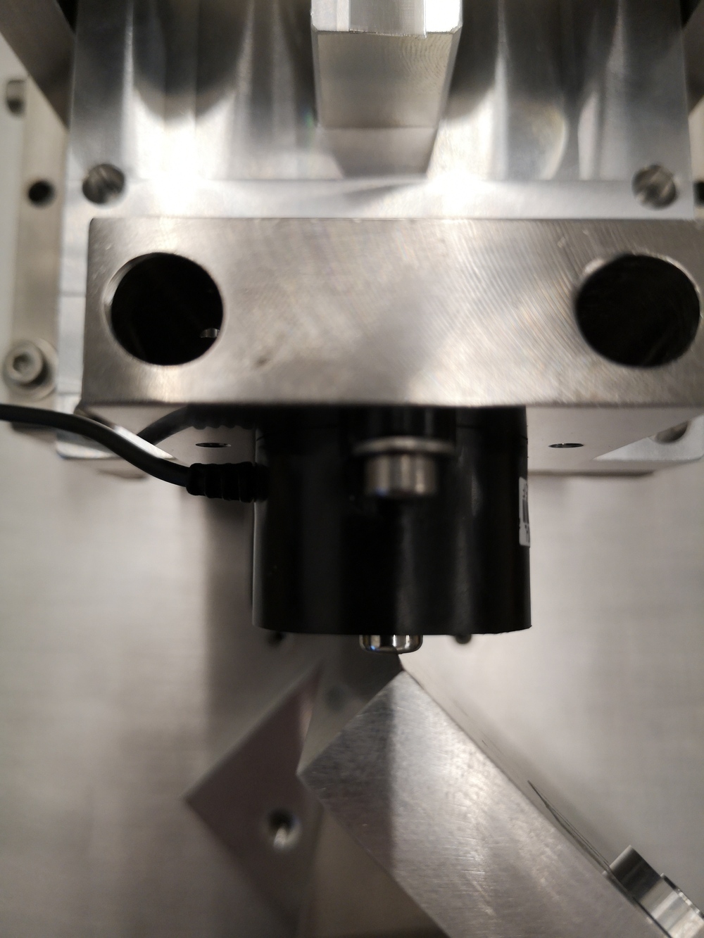
A picture of the bench used to measure the X-bending stiffness of the flexible joints is shown in Figure ref:fig:test_joints_picture_bench_overview. A closer view on flexible joint is shown in Figure ref:fig:test_joints_picture_bench_close and a zoom on the force sensor tip is shown in Figure ref:fig:test_joints_picture_bench_zoom.

The same bench used to measure the Y-bending stiffness of the flexible joint by pivoting the flexible joint by 90 degrees.

Force Sensor Calibration

Load Cells:

• FC2231-0000-0010-L
• XFL212R

There are both specified to have $\pm 1 \%$ of non-linearity over the full range.

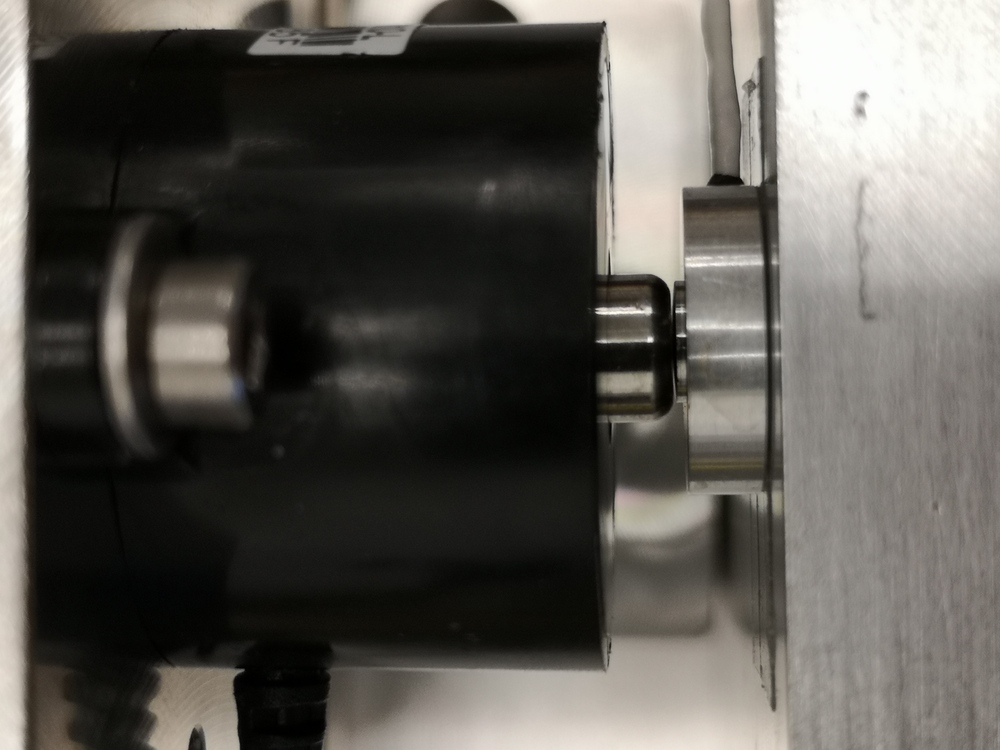
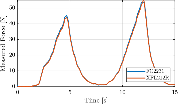
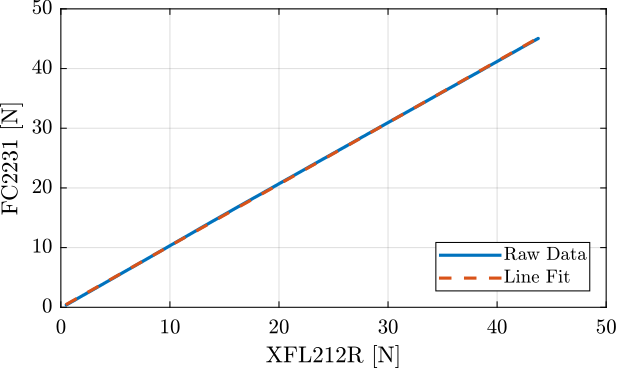
The XFL212R has a spherical interface while the FC2231 has a flat surface. Therefore, we should have a nice point contact when using the two force sensors as shown in Figure ref:fig:test_joints_force_sensor_calib.

The two force sensors are therefore measuring the exact same force, and we can compare the two measurements.

Let's load the measured force of both sensors.

%% Load measurement data
load('calibration_force_sensor.mat', 't', 'F', 'Fc')

We remove any offset such that they are both measuring no force when not in contact.

%% Remove offset
F  = F  - mean(F( t > 0.5 & t < 1.0));
Fc = Fc - mean(Fc(t > 0.5 & t < 1.0));

Measured force using both sensors as a function of time

Let's select only the first part from the moment they are in contact until the maximum force is reached.

%% Only get the first part until maximum force
F  = F( t > 1.55 & t < 4.65);
Fc = Fc(t > 1.55 & t < 4.65);

Then, let's make a linear fit between the two measured forces.

%% Make a line fit
fit_F = polyfit(Fc, F, 1);

The two forces are plotted against each other as well as the linear fit in Figure ref:fig:test_joints_force_sensor_calib_fit.

Measured two forces and linear fit

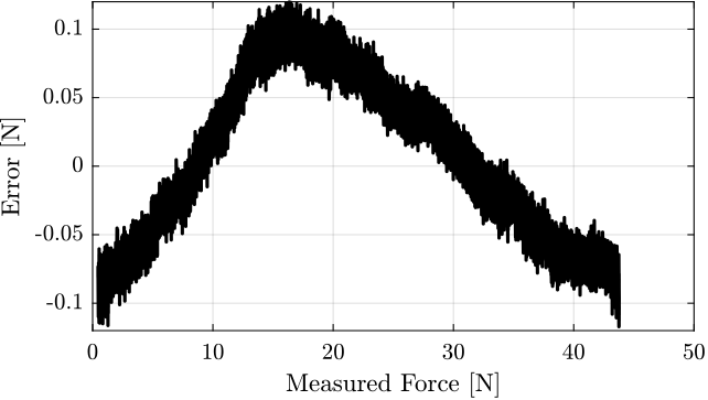
The measurement error between the two sensors is shown in Figure ref:fig:test_joints_force_sensor_calib_error. It is below 0.1N for the full measurement range.

Error in Newtons

Force Sensor Stiffness

The objective of this measurement is to estimate the stiffness of the force sensor FC2231-0000-0010-L.

To do so, a very stiff element is fixed in front of the force sensor as shown in Figure ref:fig:test_joints_meas_force_sensor_stiffness.

Then, we apply a force on the stiff element through the force sensor. We measure the deflection of the force sensor using an encoder.

Then, having the force and the deflection, we should be able to estimate the stiffness of the force sensor supposing the stiffness of the other elements are much larger.

From the documentation, the deflection of the sensor at the maximum load (50N) is 0.05mm, the stiffness is therefore foreseen to be around $1\,N/\mu m$.

Let's load the measured force as well as the measured displacement.

%% Load measurement data
load('force_sensor_stiffness_meas.mat', 't', 'F', 'd')

Some pre-processing is applied on the data.

%% Remove offset
F  = F - mean(F(t > 0.5 & t < 1.0));

%% Select important part of data
F  = F( t > 4.55 & t < 7.24);
d  = d( t > 4.55 & t < 7.24); d = d - d(1);
t  = t( t > 4.55 & t < 7.24);

The linear fit is performed.

%% Linear fit
fit_k = polyfit(F, d, 1);

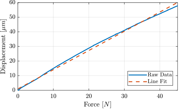
The displacement as a function of the force as well as the linear fit are shown in Figure ref:fig:test_joints_force_sensor_stiffness_fit.

Displacement as a function of the measured force

And we obtain the following stiffness:

k = 0.76 [N/um]

Analysis of one measurement

In this section is shown how the data are analysis in order to measured:

• the bending stiffness
• the bending stroke
• the stiffness once the mechanical stops are in contact

The height from the flexible joint's center and the point of application force $h$ is defined below:

h = 25e-3; % [m]

%% Load Data
load('meas_stiff_flex_1_x.mat', 't', 'F', 'd');

%% Zero the force
F = F - mean(F(t > 0.1 & t < 0.3));

%% Start measurement at t = 0.2 s
d = d(t > 0.2);
F = F(t > 0.2);
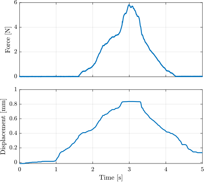
t = t(t > 0.2); t = t - t(1);

The obtained time domain measurements are shown in Figure ref:fig:test_joints_meas_bend_time.

Typical time domain measurements

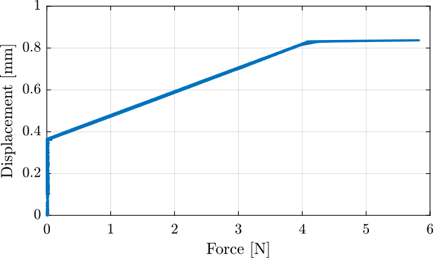
The displacement as a function of the force is then shown in Figure ref:fig:test_joints_meas_F_d.

Typical measurement of the diplacement as a function of the applied force

The bending stiffness can be estimated by computing the slope of the curve in Figure ref:fig:test_joints_meas_F_d. The bending stroke and the stiffness when touching the mechanical stop can also be estimated from the same figure.

%% Determine the linear region and region when touching the mechanical stop
% Find when the force sensor touches the flexible joint
i_l_start = find(F > 0.3, 1, 'first');
% Reset the measured diplacement at that point
d = d - d(i_l_start);
% Find then the maximum force is applied
[~, i_s_stop] = max(F);
% Linear region stops ~ when 90% of the stroke is reached
i_l_stop = find(d > 0.9*d(i_s_stop), 1, 'first');
% "Stop" region start ~1N before maximum force is applied
i_s_start = find(F > max(F)-1, 1, 'first');

%% Define variables for the two regions
F_l = F(i_l_start:i_l_stop);
d_l = d(i_l_start:i_l_stop);

F_s = F(i_s_start:i_s_stop);
d_s = d(i_s_start:i_s_stop);

%% Fit the best straight line for the two regions
fit_l = polyfit(F_l, d_l, 1);
fit_s = polyfit(F_s, d_s, 1);

%% Reset displacement based on fit
d = d - fit_l(2);
fit_s(2) = fit_s(2) - fit_l(2);
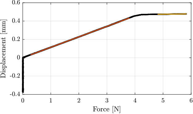
fit_l(2) = 0;

The raw data as well as the fit corresponding to the two stiffnesses are shown in Figure ref:fig:test_joints_meas_F_d_lin_fit.

Typical measurement of the diplacement as a function of the applied force with estimated linear fits

Then, the bending stroke is estimated as crossing point between the two fitted lines:

d_max = fit_l(1)*fit_s(2)/(fit_l(1) - fit_s(1));

The obtained characteristics are:

• Bending Stiffness: 5.5Nm/rad
• Bending Stiffness at stop: 173.6Nm/rad
• Bending Stroke: 18.9mrad

Bending stiffness and bending stroke of all the flexible joints

Now, let's estimate the bending stiffness and stroke for all the flexible joints.

The results are summarized in Table ref:tab:test_joints_meas_results_x_dir for the X direction and in Table ref:tab:test_joints_meas_results_y_dir for the Y direction.

	$R_{R_x}$ [Nm/rad]	$k_{R_x,s}$ [Nm/rad]	$R_{x,\text{max}}$ [mrad]
1	5.5	173.6	18.9
2	6.1	195.0	17.6
3	6.1	191.3	17.7
4	5.8	136.7	18.3
5	5.7	88.9	22.0
6	5.7	183.9	18.7
7	5.7	157.9	17.9
8	5.8	166.1	17.9
9	5.8	159.5	18.2
10	6.0	143.6	18.1
11	5.0	163.8	17.7
12	6.1	111.9	17.0
13	6.0	142.0	17.4
14	5.8	130.1	17.9
15	5.7	170.7	18.6
16	6.0	148.7	17.5

	$R_{R_y}$ [Nm/rad]	$k_{R_y,s}$ [Nm/rad]	$R_{y,\text{may}}$ [mrad]
1	5.7	323.5	17.9
2	5.9	306.0	17.2
3	6.0	224.4	16.8
4	5.7	247.3	17.8
5	5.8	250.9	13.0
6	5.8	244.5	17.8
7	5.3	214.8	18.1
8	5.8	217.2	17.6
9	5.7	225.0	17.6
10	6.0	254.7	17.3
11	4.9	261.1	18.4
12	5.9	161.5	16.7
13	6.1	227.6	16.8
14	5.9	221.3	17.8
15	5.4	241.5	17.8
16	5.3	291.1	17.7

Analysis

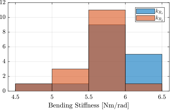
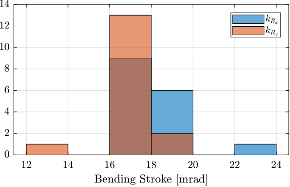
The dispersion of the measured bending stiffness is shown in Figure ref:fig:test_joints_bend_stiff_hist and of the bending stroke in Figure ref:fig:test_joints_bend_stroke_hist.

Histogram of the measured bending stiffness

Histogram of the measured bending stroke

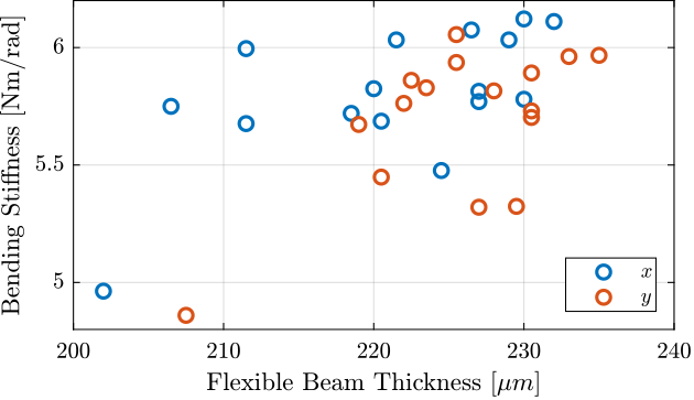
The relation between the measured beam thickness and the measured bending stiffness is shown in Figure ref:fig:test_joints_thickness_stiffness.

Measured bending stiffness as a function of the estimated flexible beam thickness

Conclusion

The measured bending stiffness and bending stroke of the flexible joints are very close to the estimated one using a Finite Element Model.

The characteristics of all the flexible joints are also quite close to each other. This should allow us to model them with unique parameters.

Conclusion

<<sec:test_joints_conclusion>>

Bibliography   ignore

Footnotes

¹The alloy used is called F16PH, also refereed as "1.4542"

---