53 KiB
Flexible Joints - Test Bench
- Introduction
- Dimensional Measurements
- Compliance Measurement Test Bench
- Bending Stiffness Measurement
- Conclusion
- Bibliography
- Footnotes
This report is also available as a pdf.
Introduction ignore
At both ends of the nano-hexapod struts, a flexible joint is used. Ideally, these flexible joints would behave as perfect spherical joints, that is to say no bending and torsional stiffness, infinite shear and axial stiffness, unlimited bending and torsional stroke, no friction, and no backlash.
Deviations from these ideal properties will impact the dynamics of the Nano-Hexapod and could limit the attainable performance. During the detailed design phase, specifications in terms of stiffness and stroke were determined and are summarized in Table ref:tab:test_joints_specs.
| Specification | FEM | |
|---|---|---|
| Axial Stiffness | $> 100\,N/\mu m$ | 94 |
| Shear Stiffness | $> 1\,N/\mu m$ | 13 |
| Bending Stiffness | $< 100\,Nm/\text{rad}$ | 5 |
| Torsion Stiffness | $< 500\,Nm/\text{rad}$ | 260 |
| Bending Stroke | $> 1\,\text{mrad}$ | 24.5 |
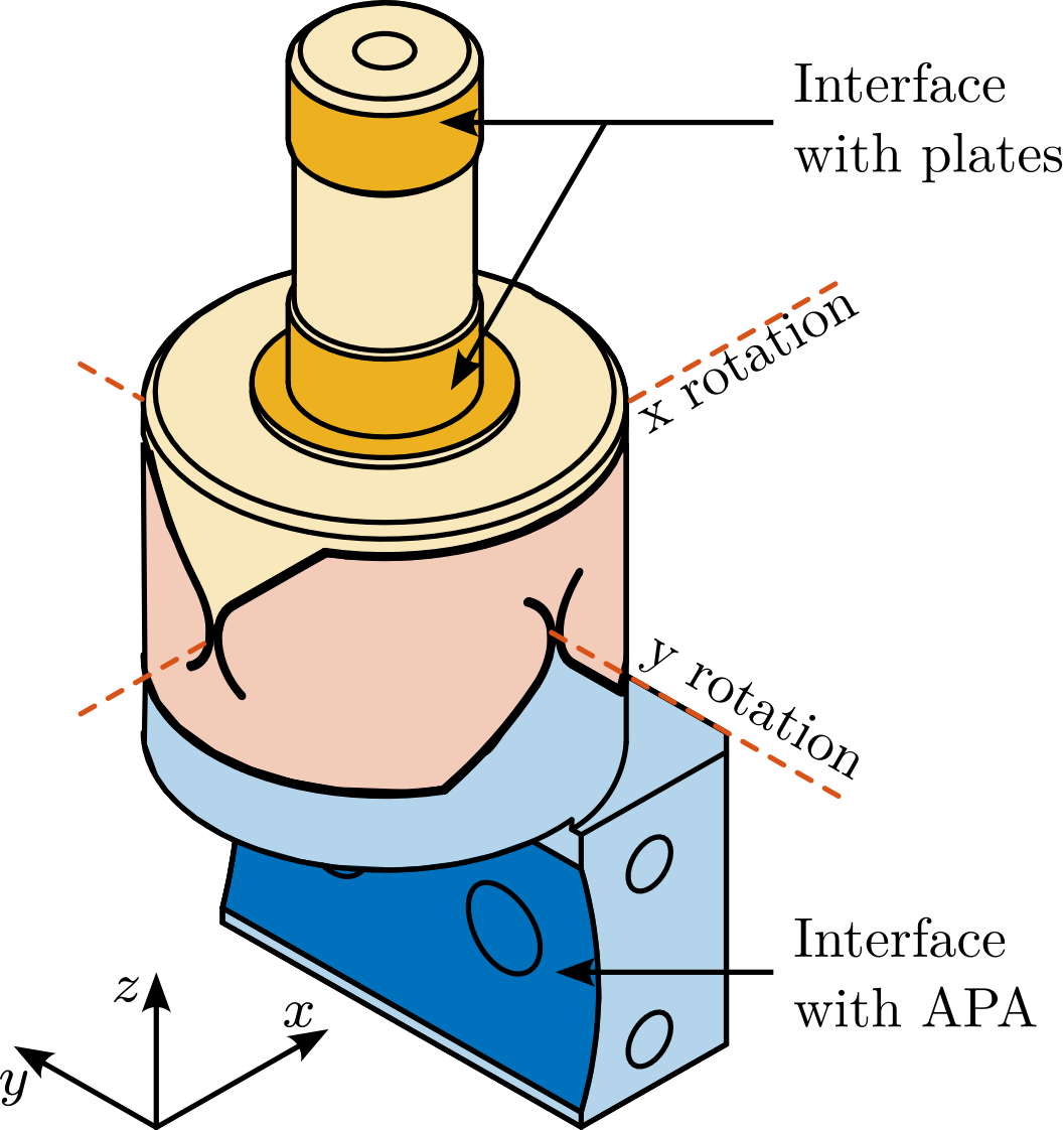
After optimization using a finite element model, the geometry shown in Figure ref:fig:test_joints_schematic has been obtained and the corresponding flexible joint characteristics are summarized in Table ref:tab:test_joints_specs. This flexible joint is a monolithic piece of stainless steel1 manufactured using wire electrical discharge machining. It serves several functions, as shown in Figure ref:fig:test_joints_iso, such as:
- Rigid interfacing with the nano-hexapod plates (yellow surfaces)
- Rigid interfacing with the amplified piezoelectric actuator (blue surface)
- Allow two rotations between the "yellow" and the "blue" interfaces. The rotation axes are represented by the dashed lines that intersect
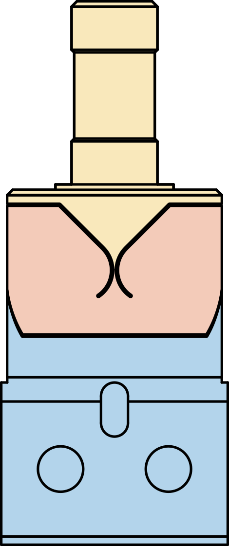
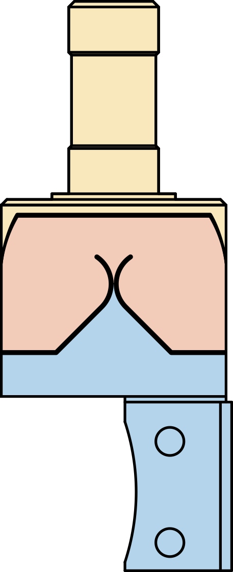
Sixteen flexible joints have been ordered (shown in Figure ref:fig:test_joints_received) such that some selection can be made for the twelve that will be used on the nano-hexapod.
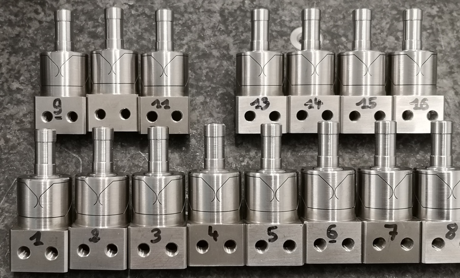
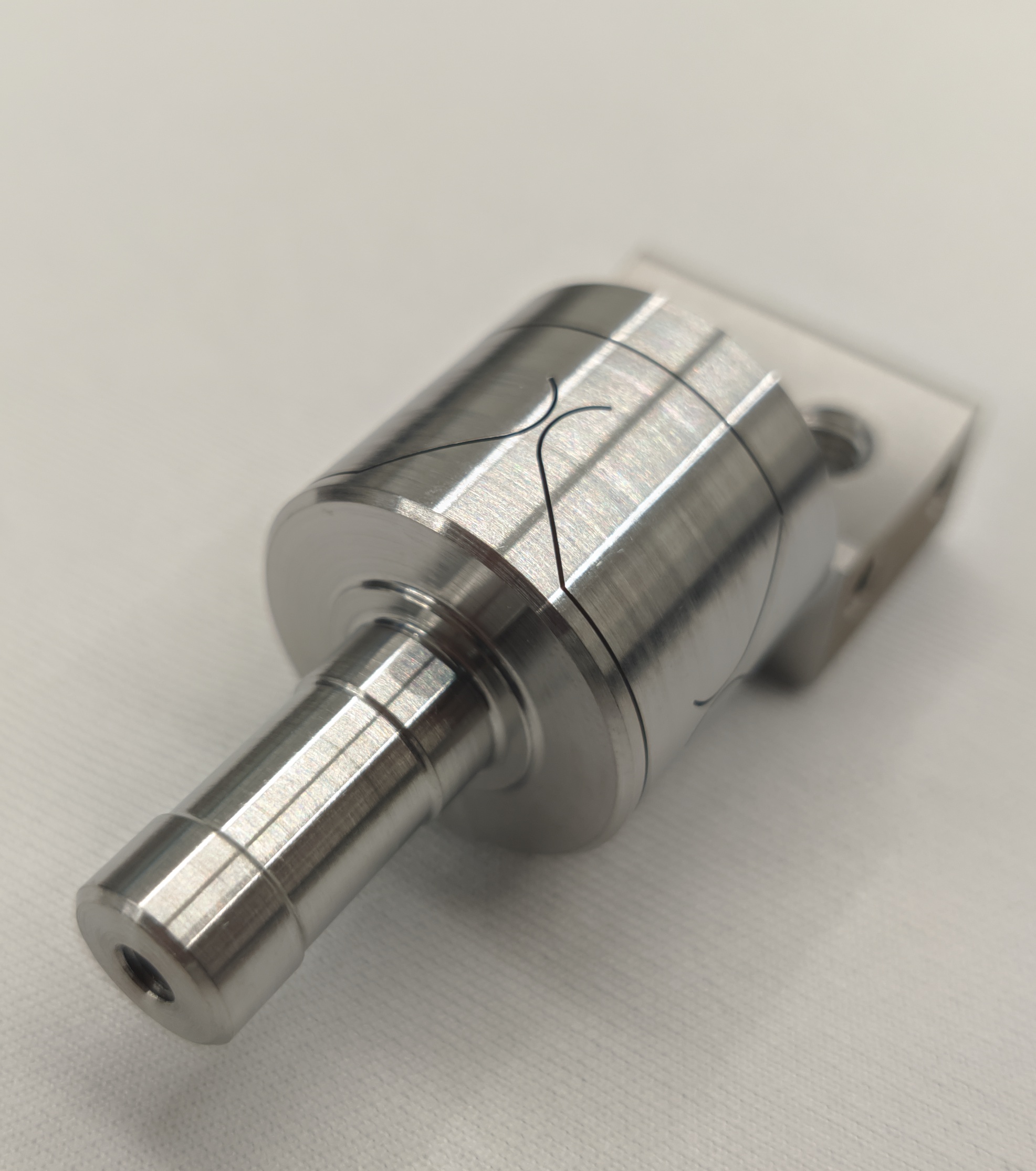
In this document, the received flexible joints are characterized to ensure that they fulfill the requirements and such that they can well be modeled.
First, the flexible joints are visually inspected, and the minimum gaps (responsible for most of the joint compliance) are measured (Section ref:sec:test_joints_flex_dim_meas). Then, a test bench was developed to measure the bending stiffness of the flexible joints. The development of this test bench is presented in Section ref:sec:test_joints_test_bench_desc, including a noise budget and some requirements in terms of instrumentation. The test bench is then used to measure the bending stiffnesses of all the flexible joints. Results are shown in Section ref:sec:test_joints_bending_stiffness_meas
Dimensional Measurements
<<sec:test_joints_flex_dim_meas>>
Measurement Bench
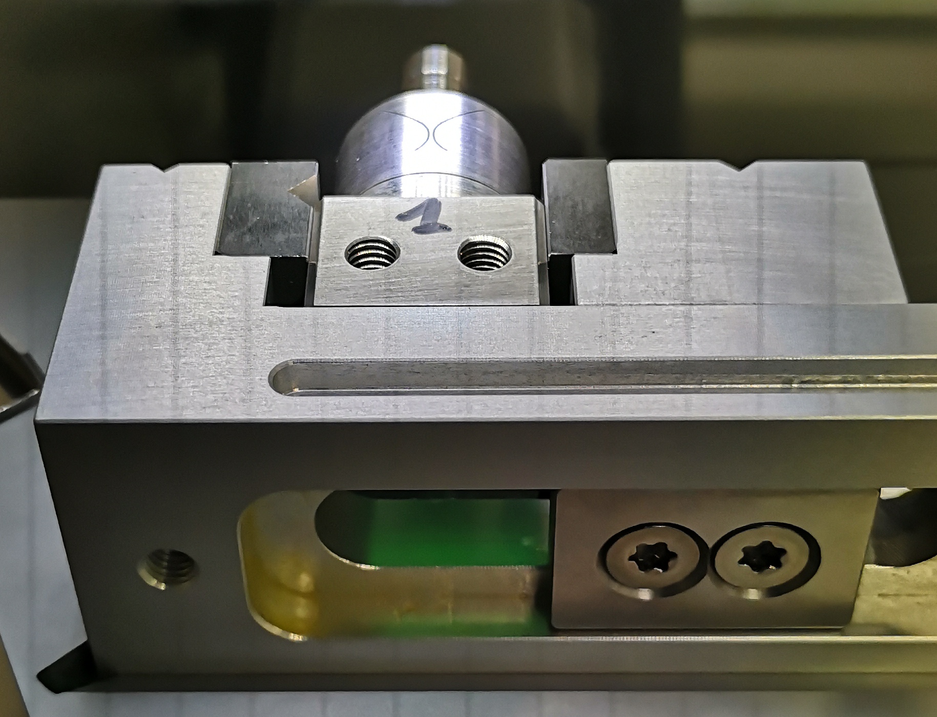
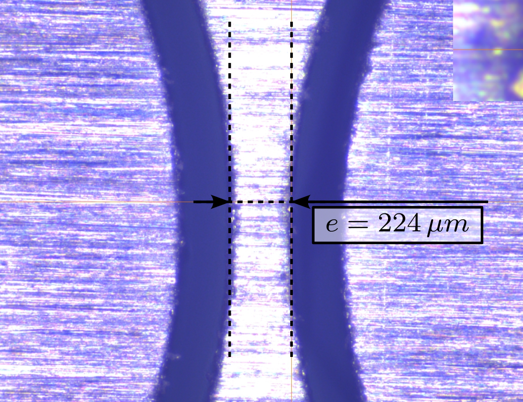
Two dimensions are critical for the bending stiffness of the flexible joints. These dimensions can be measured using a profilometer. The dimensions of the flexible joint in the Y-Z plane will contribute to the X-bending stiffness, whereas the dimensions in the X-Z plane will contribute to the Y-bending stiffness.
The setup used to measure the dimensions of the "X" flexible beam is shown in Figure ref:fig:test_joints_profilometer_setup. What is typically observed is shown in Figure ref:fig:test_joints_profilometer_image. It is then possible to estimate the dimension of the flexible beam with an accuracy of $\approx 5\,\mu m$,
Measurement Results
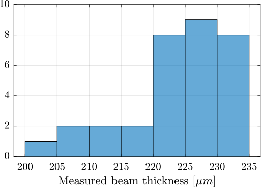
The specified flexible beam thickness (gap) is $250\,\mu m$. Four gaps are measured for each flexible joint (2 in the $x$ direction and 2 in the $y$ direction). The "beam thickness" is then estimated as the mean between the gaps measured on opposite sides.
A histogram of the measured beam thicknesses is shown in Figure ref:fig:test_joints_size_hist. The measured thickness is less than the specified value of $250\,\mu m$, but this optical method may not be very accurate because the estimated gap can depend on the lighting of the part and of its proper alignment.
However, what is more important than the true value of the thickness is the consistency between all flexible joints.
Bad flexible joints
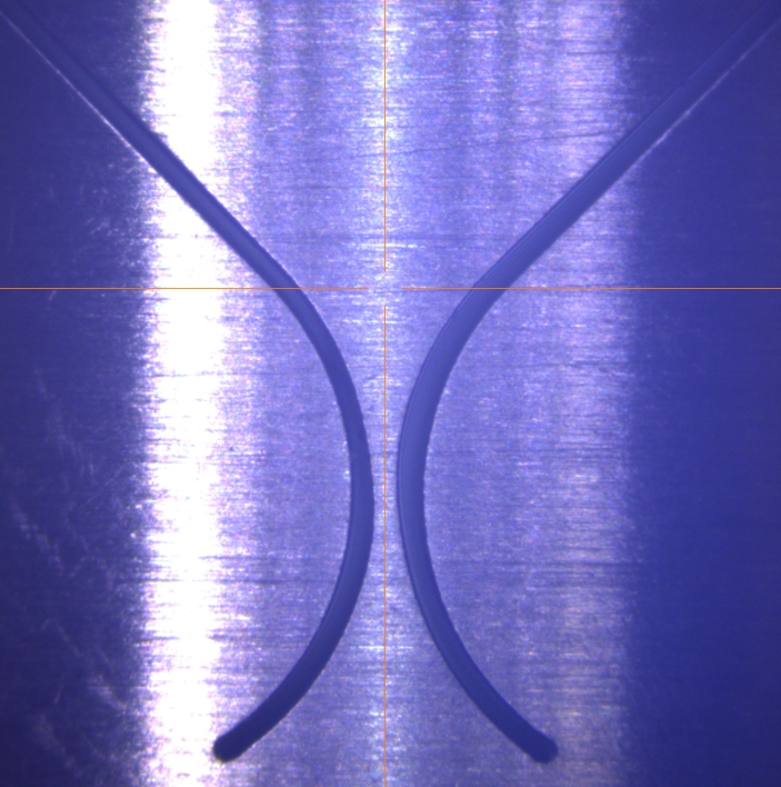
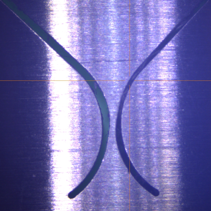
Using this profilometer allowed to detect flexible joints with manufacturing defects such as non-symmetrical shapes (see Figure ref:fig:test_joints_bad_shape) or flexible joints with machining chips stuck in the gap (see Figure ref:fig:test_joints_bad_chips).
Compliance Measurement Test Bench
<<sec:test_joints_test_bench_desc>>
Introduction ignore
The most important characteristic of the flexible joint to be measured is its bending stiffness $k_{R_x} \approx k_{R_y}$.
To estimate the bending stiffness, the basic idea is to apply a torque $T_{x}$ to the flexible joints and to measure its angular deflection $\theta_{x}$. The bending stiffness can then be computed from equation eqref:eq:test_joints_bending_stiffness.
\begin{equation}\label{eq:test_joints_bending_stiffness} \boxed{kR_x = \frac{T_x}{θ_x}, \quad kR_y = \frac{T_y}{θ_y}}
\end{equation}
Measurement principle
<<ssec:test_joints_meas_principle>>
Torque and Rotation measurement
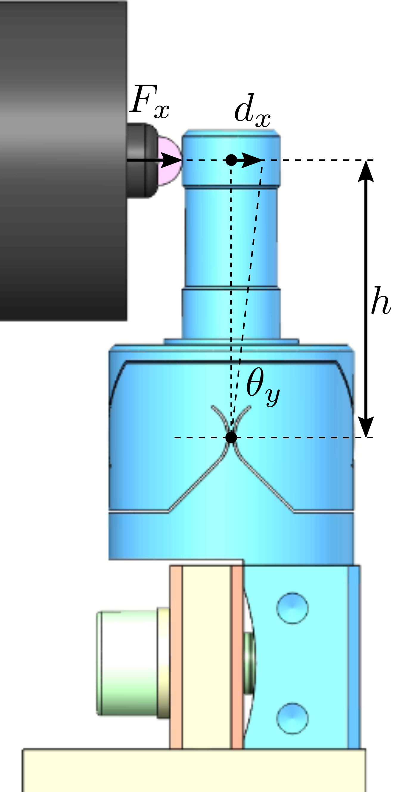
To apply torque $T_{y}$ between the two mobile parts of the flexible joint, a known "linear" force $F_{x}$ can be applied instead at a certain distance $h$ with respect to the rotation point. In this case, the equivalent applied torque can be estimated from equation eqref:eq:test_joints_force_torque_distance. Note that the application point of the force should be sufficiently far from the rotation axis such that the resulting bending motion is much larger than the displacement due to shear. Such effects are studied in Section ref:ssec:test_joints_error_budget.
\begin{equation}\label{eq:test_joints_force_torque_distance} T_y = h F_x, \quad T_x = h F_y
\end{equation}
Similarly, instead of directly measuring the bending motion $\theta_y$ of the flexible joint, its linear motion $d_x$ at a certain distance $h$ from the rotation points is measured. The equivalent rotation is estimated from eqref:eq:test_joints_rot_displ.
\begin{equation}\label{eq:test_joints_rot_displ} θ_y = tan-1≤ft(\frac{d_x}{h}\right) ≈ \frac{d_x}{h}, \quad θ_x = tan-1 ≤ft( \frac{d_y}{h} \right) ≈ \frac{d_y}{h}
\end{equation}
Then, the bending stiffness can be estimated from eqref:eq:test_joints_stiff_displ_force.
\begin{subequations}\label{eq:test_joints_stiff_displ_force}
\begin{align} k_{R_x} &= \frac{T_x}{\theta_x} = \frac{h F_y}{\tan^{-1}\left( \frac{d_y}{h} \right)} \approx h^2 \frac{F_y}{d_y} \\ k_{R_y} &= \frac{T_y}{\theta_y} = \frac{h F_x}{\tan^{-1}\left( \frac{d_x}{h} \right)} \approx h^2 \frac{F_x}{d_x} \end{align}\end{subequations}
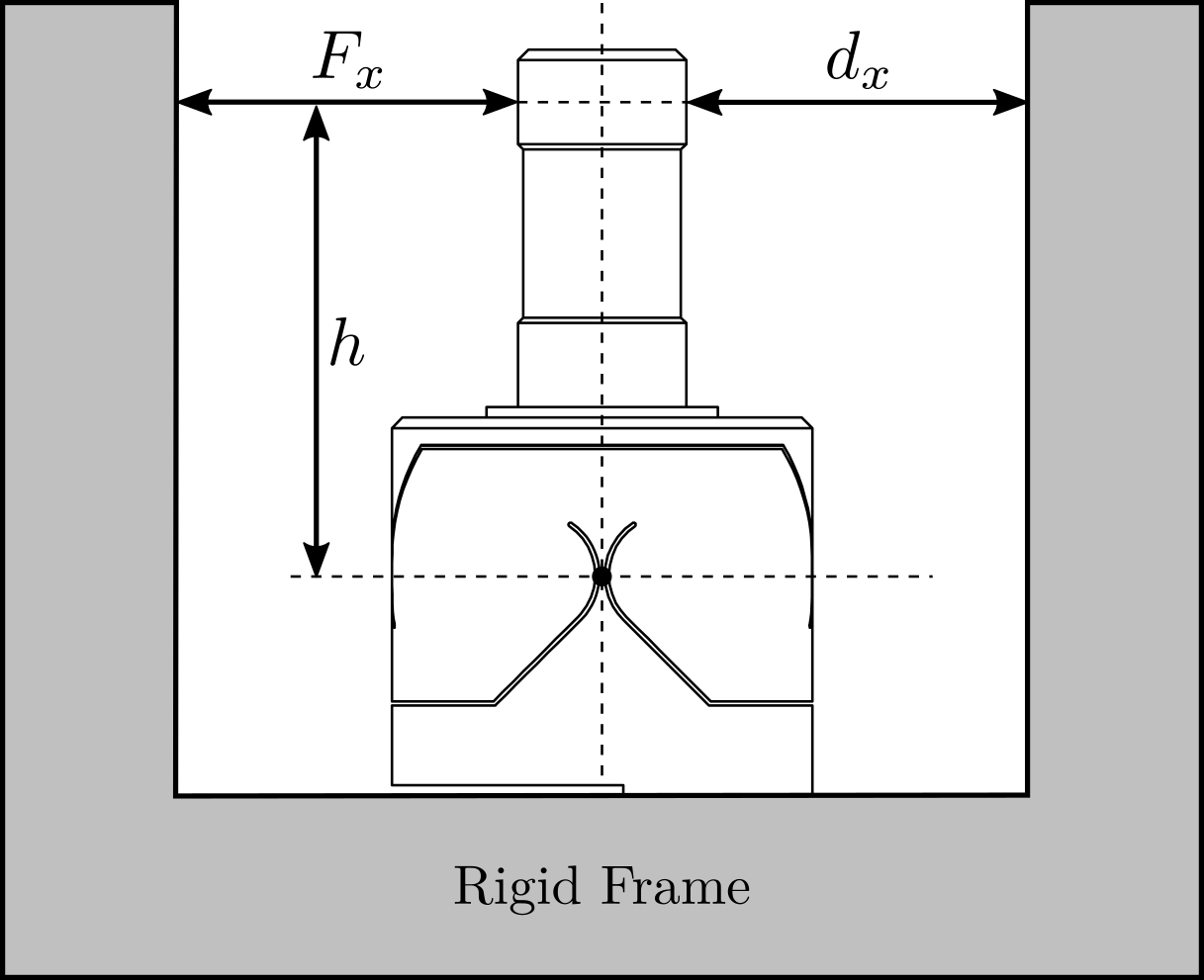
The working principle of the measurement bench is schematically shown in Figure ref:fig:test_joints_bench_working_principle. One part of the flexible joint is fixed to a rigid frame while a (known) force $F_x$ is applied to the other side of the flexible joint. The deflection of the joint $d_x$ is measured using a displacement sensor.
Required external applied force
The bending stiffness is foreseen to be $k_{R_y} \approx k_{R_x} \approx 5\,\frac{Nm}{rad}$ and its stroke $\theta_{y,\text{max}}\approx \theta_{x,\text{max}}\approx 25\,mrad$. The height between the flexible point (center of the joint) and the point where external forces are applied is $h = 22.5\,mm$ (see Figure ref:fig:test_joints_bench_working_principle).
%% Parameters for study
kRx = 5;       % Bending Stiffness [Nm/rad]
Rxmax = 25e-3; % Bending Stroke [rad]
h = 22.5e-3;     % Height [m]

%% Estimation of the force to test the full stroke
Fxmax = kRx*Rxmax/h; % Force to induce maximum stroke [N]
The bending $\theta_y$ of the flexible joint due to the force $F_x$ is given by equation eqref:eq:test_joints_deflection_force.
\begin{equation}\label{eq:test_joints_deflection_force} θ_y = \frac{T_y}{kR_y} = \frac{F_x h}{kR_y}
\end{equation}
Therefore, the force that must be applied to test the full range of the flexible joints is given by equation eqref:eq:test_joints_max_force. The measurement range of the force sensor should then be higher than $5.5\,N$.
\begin{equation}\label{eq:test_joints_max_force} F_{x,\text{max}} = \frac{kR_y θ_{y,\text{max}}}{h} ≈ 5.5\,N
\end{equation}
Required actuator stroke and sensors range
The flexible joint is designed to allow a bending motion of $\pm 25\,mrad$. The corresponding stroke at the location of the force sensor is given by eqref:eq:test_joints_max_stroke. To test the full range of the flexible joint, the means of applying a force (explained in the next section) should allow a motion of at least $0.5\,mm$. Similarly, the measurement range of the displacement sensor should also be higher than $0.5\,mm$.
\begin{equation}\label{eq:test_joints_max_stroke} d_{x,\text{max}} = h tan(R_{x,\text{max}}) ≈ 0.5\,mm
\end{equation}
%% Estimated maximum stroke [m]
dxmax = h*tan(Rxmax);
Force and Displacement measurements
To determine the applied force, a load cell will be used in series with the mechanism that applied the force. The measured deflection of the flexible joint will be indirectly estimated from the displacement of the force sensor itself (see Section ref:ssec:test_joints_test_bench). Indirectly measuring the deflection of the flexible joint induces some errors because of the limited stiffness between the force sensor and the displacement sensor. Such an effect will be estimated in the error budget (Section ref:ssec:test_joints_error_budget)
Error budget
<<ssec:test_joints_error_budget>>
Introduction ignore
To estimate the accuracy of the measured bending stiffness that can be obtained using this measurement principle, an error budget is performed.
Based on equation eqref:eq:test_joints_stiff_displ_force, several errors can affect the accuracy of the measured bending stiffness:
- Errors in the measured torque $M_x, M_y$: this is mainly due to inaccuracies in the load cell and of the height estimation $h$
- Errors in the measured bending motion of the flexible joints $\theta_x, \theta_y$: errors from limited shear stiffness, from the deflection of the load cell itself, and inaccuracy of the height estimation $h$
If only the bending stiffness is considered, the induced displacement is described by eqref:eq:test_joints_dbx.
\begin{equation}\label{eq:test_joints_dbx} dx,b = h tan(θ_y) = h tan≤ft( \frac{F_x ⋅ h}{kR_y} \right)
\end{equation}
Effect of Shear
The applied force $F_x$ will induce some shear $d_{x,s}$ which is described by eqref:eq:test_joints_shear_displ with $k_s$ the shear stiffness of the flexible joint.
\begin{equation}\label{eq:test_joints_shear_displ} dx,s = \frac{F_x}{k_s}
\end{equation}
The measured displacement $d_x$ is affected shear, as shown in equation eqref:eq:test_joints_displ_shear.
\begin{equation}\label{eq:test_joints_displ_shear} d_x = dx,b + dx,s = h tan≤ft( \frac{F_x ⋅ h}{kR_y} \right) + \frac{F_x}{k_s} ≈ F_x ≤ft( \frac{h^2}{kR_y} + \frac{1}{k_s} \right)
\end{equation}
The estimated bending stiffness $k_{\text{est}}$ then depends on the shear stiffness eqref:eq:test_joints_error_shear.
\begin{equation}\label{eq:test_joints_error_shear} k_{R_y,\text{est}} = h^2 \frac{F_x}{d_x} ≈ kR_y \frac{1}{1 + \frac{kR_y}{k_s h^2}} ≈ kR_y \Bigl( 1 - _brace{\frac{kR_y}{k_s h^2}}_{εs} \Bigl)
\end{equation}
With an estimated shear stiffness $k_s = 13\,N/\mu m$ from the finite element model and an height $h=25\,mm$, the estimation errors of the bending stiffness due to shear is $\epsilon_s < 0.1\,\%$
%% Estimated error due to shear
epsilon_s = 100*abs(1-1/(1 + kb/(ks*h^2))); % Error in %
Effect of load cell limited stiffness
As explained in the previous section, because the measurement of the flexible joint deflection is indirectly performed with the encoder, errors will be made if the load cell experiences some compression.
Suppose the load cell has an internal stiffness $k_f$, the same reasoning that was made for the effect of shear can be applied here. The estimation error of the bending stiffness due to the limited stiffness of the load cell is then described by eqref:eq:test_joints_error_load_cell_stiffness.
\begin{equation}\label{eq:test_joints_error_load_cell_stiffness} k_{R_y,\text{est}} = h^2 \frac{F_x}{d_x} ≈ kR_y \frac{1}{1 + \frac{kR_y}{k_F h^2}} ≈ kR_y \Bigl( 1 - _brace{\frac{kR_y}{k_F h^2}}ε_f \Bigl)
\end{equation}
With an estimated load cell stiffness of $k_f \approx 1\,N/\mu m$ (from the documentation), the errors due to the load cell limited stiffness is around $\epsilon_f = 1\,\%$.
%% Estimated error due to limited load cell stiffness
kF = 50/0.05e-3; % Estimated load cell stiffness [N/m]
epsilon_f = 100*abs(1-1/(1 + kb/(kF*h^2))); % Error in %
Estimation error due to height estimation error
Now consider an error $\delta h$ in the estimation of the height $h$ as described by eqref:eq:test_joints_est_h_error.
\begin{equation}\label{eq:test_joints_est_h_error} h_{\text{est}} = h + δ h
\end{equation}
The computed bending stiffness will be eqref:eq:test_joints_stiffness_height_error.
\begin{equation}\label{eq:test_joints_stiffness_height_error} k_{R_y, \text{est}} ≈ h_{\text{est}}^2 \frac{F_x}{d_x} ≈ kR_y \Bigl( 1 + _brace{2 \frac{δ h}{h} + \frac{δ h ^2}{h^2}}ε_h \Bigl)
\end{equation}
The height estimation is foreseen to be accurate to within $|\delta h| < 0.4\,mm$ which corresponds to a stiffness error $\epsilon_h < 3.5\,\%$.
Estimation error due to force and displacement sensors accuracy
An optical encoder is used to measure the displacement (see Section ref:ssec:test_joints_test_bench) whose maximum non-linearity is $40\,nm$. As the measured displacement is foreseen to be $0.5\,mm$, the error $\epsilon_d$ due to the encoder non-linearity is negligible $\epsilon_d < 0.01\,\%$.
The accuracy of the load cell is specified at $1\,\%$ and therefore, estimation errors of the bending stiffness due to the limited load cell accuracy should be $\epsilon_F < 1\,\%$
Conclusion
The different sources of errors are summarized in Table ref:tab:test_joints_error_budget. The most important source of error is the estimation error of the distance between the flexible joint rotation axis and its contact with the force sensor. An overall accuracy of $\approx 5\,\%$ can be expected with this measurement bench, which should be sufficient for an estimation of the bending stiffness of the flexible joints.
| Effect | Error |
|---|---|
| Shear effect | $\epsilon_s < 0.1\,\%$ |
| Load cell compliance | $\epsilon_f = 1\,\%$ |
| Height error | $\epsilon_h < 3.5\,\%$ |
| Displacement sensor | $\epsilon_d < 0.01\,\%$ |
| Force sensor | $\epsilon_F < 1\,\%$ |
Mechanical Design
<<ssec:test_joints_test_bench>>
As explained in Section ref:ssec:test_joints_meas_principle, the flexible joint's bending stiffness is estimated by applying a known force to the flexible joint's tip and by measuring its deflection at the same point.
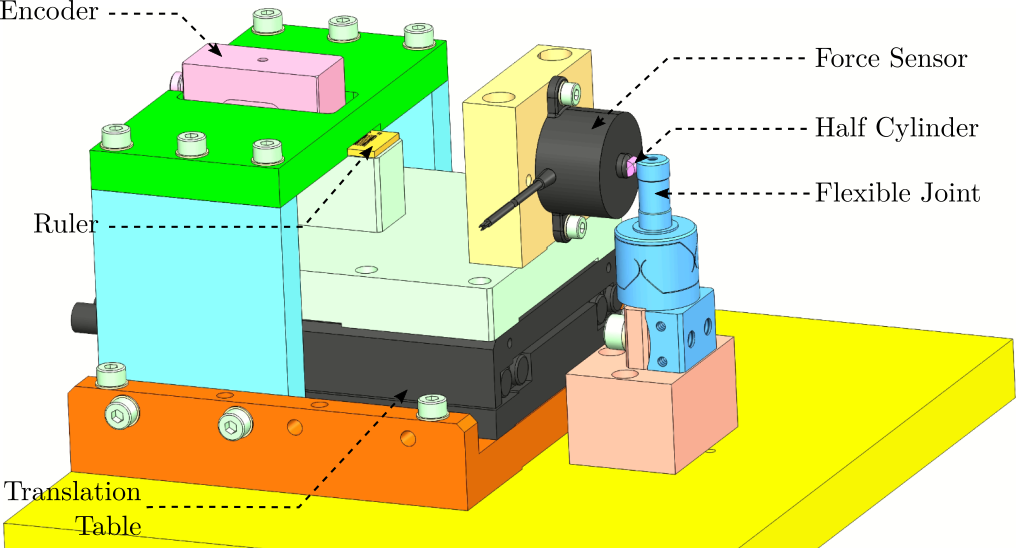
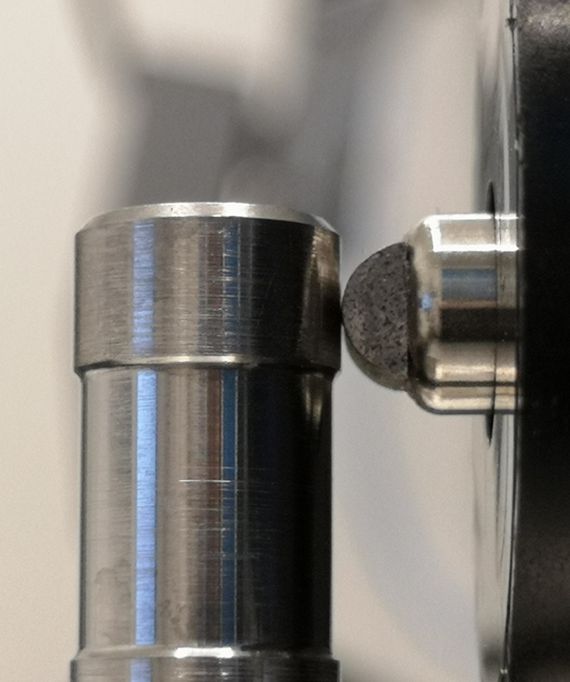
The force is applied using a load cell2 such that the applied force to the flexible joint's tip is directly measured. To control the height and direction of the applied force, a cylinder cut in half is fixed at the tip of the force sensor (pink element in Figure ref:fig:test_joints_bench_side) that initially had a flat surface. Doing so, the contact between the flexible joint cylindrical tip and the force sensor is a point (intersection of two cylinders) at a precise height, and the force is applied in a known direction. To translate the load cell at a constant height, it is fixed to a translation stage3 which is moved by hand.
Instead of measuring the displacement directly at the tip of the flexible joint (with a probe or an interferometer for instance), the displacement of the load cell itself is measured. To do so, an encoder4 is used, which measures the motion of a ruler. This ruler is fixed to the translation stage in line (i.e. at the same height) with the application point to reduce Abbe errors (see Figure ref:fig:test_joints_bench_overview).
The flexible joint can be rotated by $90^o$ in order to measure the bending stiffness in the two directions. The obtained CAD design of the measurement bench is shown in Figure ref:fig:test_joints_bench_overview while a zoom on the flexible joint with the associated important quantities is shown in Figure ref:fig:test_joints_bench_side.
Bending Stiffness Measurement
<<sec:test_joints_bending_stiffness_meas>>
Introduction ignore
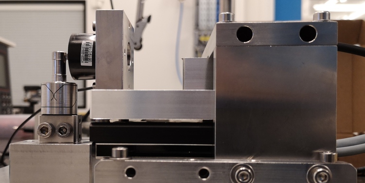
A picture of the bench used to measure the X-bending stiffness of the flexible joints is shown in Figure ref:fig:test_joints_picture_bench_overview. A closer view of the force sensor tip is shown in Figure ref:fig:test_joints_picture_bench_zoom.
Load Cell Calibration
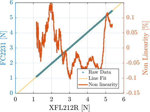
In order to estimate the measured errors of the load cell "FC2231", it is compared against another load cell5. The two load cells are measured simultaneously while they are pushed against each other (see Figure ref:fig:test_joints_force_sensor_calib_picture). The contact between the two load cells is well defined as one has a spherical interface and the other has a flat surface.
The measured forces are compared in Figure ref:fig:test_joints_force_sensor_calib_fit. The gain mismatch between the two load cells is approximately $4\,\%$ which is higher than that specified in the data sheets. However, the estimated non-linearity is bellow $0.2\,\%$ for forces between $1\,N$ and $5\,N$.
%% Force Sensor Calibration
% Load measurement data
load('calibration_force_sensor.mat', 't', 'F', 'Fc')

% Remove any offset such that they are both measuring no force when not in contact.
F  = F  - mean(F( t > 0.5 & t < 1.0)); % FC2231 [N]
Fc = Fc - mean(Fc(t > 0.5 & t < 1.0)); % XFL212R [N]

% Only get useful stroke
F  = F( t > 2 & t < 2.2);
Fc = Fc(t > 2 & t < 2.2);
t  = t( t > 2 & t < 2.2);

% Make a line fit
fit_F = polyfit(Fc, F, 1);

% Estimate the gain mismatch
F_gain_mismatch = 100*(1 - fit_F(1)); % in %

% Estimate non-linearity of the sensors
F_non_linearity = 100*(F - (Fc*fit_F(1) + fit_F(2)))./Fc; % in %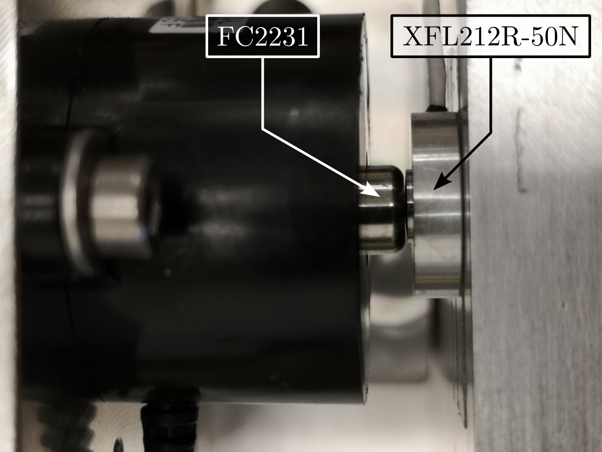
Load Cell Stiffness
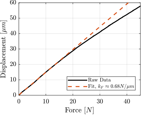
The objective of this measurement is to estimate the stiffness $k_F$ of the force sensor. To do so, a stiff element (much stiffer than the estimated $k_F \approx 1\,N/\mu m$) is mounted in front of the force sensor, as shown in Figure ref:fig:test_joints_meas_force_sensor_stiffness_picture. Then, the force sensor is pushed against this stiff element while the force sensor and the encoder displacement are measured. The measured displacement as a function of the measured force is shown in Figure ref:fig:test_joints_force_sensor_stiffness_fit. The load cell stiffness can then be estimated by computing a linear fit and is found to be $k_F \approx 0.68\,N/\mu m$.
%% Estimaetd load cell stiffness
% Load measurement data
load('force_sensor_stiffness_meas.mat', 't', 'F', 'd')

% Remove offset
F  = F - mean(F(t > 0.5 & t < 1.0));

% Select important part of data
F  = F( t > 4.55 & t < 7.24);
d  = d( t > 4.55 & t < 7.24); d = d - d(1);
t  = t( t > 4.55 & t < 7.24);

% Linear fit
fit_k = polyfit(F(F<10), d(F<10), 1);
Bending Stiffness estimation
The actual stiffness is now estimated by manually moving the translation stage from a start position where the force sensor is not yet in contact with the flexible joint to a position where the flexible joint is on its mechanical stop.
The measured force and displacement as a function of time are shown in Figure ref:fig:test_joints_meas_bend_time. Three regions can be observed: first, the force sensor tip is not in contact with the flexible joint and the measured force is zero; then, the flexible joint deforms linearly; and finally, the flexible joint comes in contact with the mechanical stop.
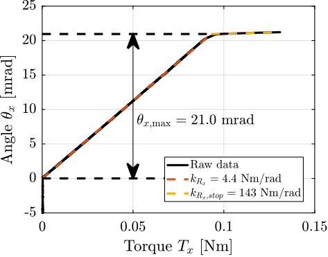
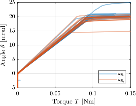
The angular motion $\theta_{y}$ computed from the displacement $d_x$ is displayed as function of the measured torque $T_{y}$ in Figure ref:fig:test_joints_meas_F_d_lin_fit. The bending stiffness of the flexible joint can be estimated by computing the slope of the curve in the linear regime (red dashed line) and is found to be $k_{R_y} = 4.4\,Nm/\text{rad}$. The bending stroke can also be estimated as shown in Figure ref:fig:test_joints_meas_F_d_lin_fit and is found to be $\theta_{y,\text{max}} = 20.9\,\text{mrad}$.
%% Estimate the bending stiffness and stroke from the measurement - First Flexible joint
% Load Measured Data for first flexible joint
load('meas_stiff_flex_1_x.mat', 't', 'F', 'd');

% Start measurement at t = 0.2 s
d = d(t > 0.2);
F = F(t > 0.2);
t = t(t > 0.2); t = t - t(1);

% Zero the force
F = F - mean(F(t < 0.2));

% Find when the force sensor touches the flexible joint
i_l_start = find(F > 0.3, 1, 'first');

% Compute torque and angular displacement
h = 22.5e-3; % Height [m]
Tx = h * F; % Applied torque in [Nm]
thetax = atan2(d - d(i_l_start), h); % Measured angle in [rad]

% Find then the maximum torque is applied
[~, i_s_stop] = max(Tx);
% Linear region stops ~ when 90% of the stroke is reached
i_l_stop = find(thetax > 0.9*thetax(i_s_stop), 1, 'first');
% Mechanical "Stop" region start ~20Nmm before maximum torque is applied
i_s_start = find(Tx > max(Tx)-20e-3, 1, 'first');

% Linear fit in the "linear" region
fit_l = polyfit(Tx(i_l_start:i_l_stop), thetax(i_l_start:i_l_stop), 1);

% Linear fit in the "mechanical stop" region
fit_s = polyfit(Tx(i_s_start:i_s_stop), thetax(i_s_start:i_s_stop), 1);

% Reset displacement more precisely based on fit
thetax = thetax - fit_l(2);
fit_s(2) = fit_s(2) - fit_l(2);
fit_l(2) = 0;

%% Estimation of the bending stiffness
kRx_l = 1/fit_l(1); % Bending Stiffness [Nm/rad]
kRx_s = 1/fit_s(1); % Mechanical "Stop" Stiffness [Nm/rad]

%% Estimation of the bending stroke
% This is done by finding the intersection of the two linear fits
theta_max = fit_l(1)*fit_s(2)/(fit_l(1) - fit_s(1)); % Maximum angular stroke [rad]
Tx_at_theta_max = (fit_s(2) - fit_l(2))/(fit_l(1) - fit_s(1));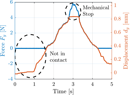
Measured flexible joint stiffness
The same measurement was performed for all the 16 flexible joints, both in the $x$ and $y$ directions. The measured angular motion as a function of the applied torque is shown in Figure ref:fig:test_joints_meas_bending_all_raw_data for the 16 flexible joints. This gives a first idea of the dispersion of the measured bending stiffnesses (i.e. slope of the linear region) and of the angular stroke.
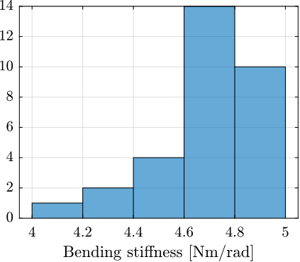
A histogram of the measured bending stiffnesses is shown in Figure ref:fig:test_joints_bend_stiff_hist. Most of the bending stiffnesses are between $4.6\,Nm/rad$ and $5.0\,Nm/rad$.
Conclusion
The measured bending stiffness and bending stroke of the flexible joints are very close to the estimated one using a Finite Element Model ($k_{R_x} = k_{R_y} = 5\,Nm/\text{rad}$). The characteristics of the flexible joints are also quite close to each other. This should allow us to model them using unique parameters.
Conclusion
<<sec:test_joints_conclusion>>
The flexible joints are a key element of the nano-hexapod. Careful dimensional measurements (Section ref:sec:test_joints_flex_dim_meas) allowed for the early identification of faulty flexible joints. This was crucial in preventing potential complications that could have arisen from the installation of faulty joints on the nano-hexapod.
A dedicated test bench was developed to asses the bending stiffness of the flexible joints. Through meticulous error analysis and budgeting, a satisfactory level of measurement accuracy could be guaranteed. The measured bending stiffness values exhibited good agreement with the predictions from the finite element model These measurements are helpful for refining the model of the flexible joints, thereby enhancing the overall accuracy of the nano-hexapod model. Furthermore, the data obtained from these measurements have provided the necessary information to select the most suitable flexible joints for the nano-hexapod, ensuring optimal performance.
Bibliography ignore
Footnotes
5XFL212R-50N from TE Connectivity. The measurement range is $50\,N$. The specified accuracy is $1\,\%$ of the full range 4Resolute\texttrademark{} encoder with $1\,nm$ resolution and $\pm 40\,nm$ maximum non-linearity 3V-408 PIMag\textsuperscript{\textregistered} linear stage is used. Crossed rollers are used to guide the motion. 2The load cell is FC22 from TE Connectivity. The measurement range is $50\,N$. The specified accuracy is $1\,\%$ of the full range 1The alloy used is called F16PH, also refereed as "1.4542"