phd-test-bench-apa/test-bench-apa.org

Test Bench - Amplified Piezoelectric Actuator

• Introduction
• First Basic Measurements
  • Introduction
  • Geometrical Measurements
  • Electrical Measurements
  • Stroke and Hysteresis Measurement
  • Flexible Mode Measurement
  • Conclusion
• Dynamical measurements
  • Introduction
  • Hysteresis
  • Axial stiffness
  • Dynamics
  • Effect of the resistor on the IFF Plant
  • Integral Force Feedback
  • Conclusion
• APA300ML - 2 Degrees of Freedom Model
  • Introduction
  • Two Degrees of Freedom APA Model
  • Tuning of the APA model
  • Obtained Dynamics
  • Conclusion
• APA300ML - Super Element
  • Introduction
  • Extraction of the super-element
  • Identification of the Actuator and Sensor constants
  • Comparison of the obtained dynamics
  • Conclusion
• Conclusion
• Bibliography
• Footnotes

---

This report is also available as a pdf.

---

Introduction   ignore

Picture of 5 out of the 7 received APA300ML

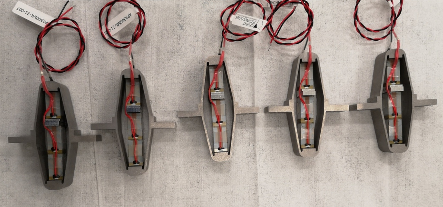
The first goal is to characterize the APA300ML in terms of:

• The, geometric features, electrical capacitance, stroke, hysteresis, spurious resonances. This is performed in Section ref:sec:test_apa_basic_meas.
• The dynamics from the generated DAC voltage (going to the voltage amplifiers and then applied on the actuator stacks) to the induced displacement, and to the measured voltage by the force sensor stack. Also the "actuator constant" and "sensor constant" are identified. This is done in Section ref:sec:test_apa_dynamics.
• Compare the measurements with the two Simscape models: 2DoF (Section ref:sec:test_apa_model_2dof) Super-Element (Section ref:sec:test_apa_model_flexible)

Sections	Matlab File
Section ref:sec:test_apa_basic_meas	test_apa_1_basic_meas.m
Section ref:sec:test_apa_dynamics	test_apa_2_dynamics.m
Section ref:sec:test_apa_model_2dof	test_apa_3_model_2dof.m
Section ref:sec:test_apa_model_flexible	test_apa_4_model_flexible.m

First Basic Measurements

<<sec:test_apa_basic_meas>>

Introduction   ignore

Before using the measurement bench to characterize the APA300ML, first simple measurements are performed:

• Section ref:ssec:test_apa_geometrical_measurements: the geometric tolerances of the interface planes are checked
• Section ref:ssec:test_apa_electrical_measurements: the capacitance of the piezoelectric stacks is measured
• Section ref:ssec:test_apa_stroke_measurements: the stroke of each APA is measured
• Section ref:ssec:test_apa_spurious_resonances: the "spurious" resonances of the APA are investigated

Geometrical Measurements

<<ssec:test_apa_geometrical_measurements>>

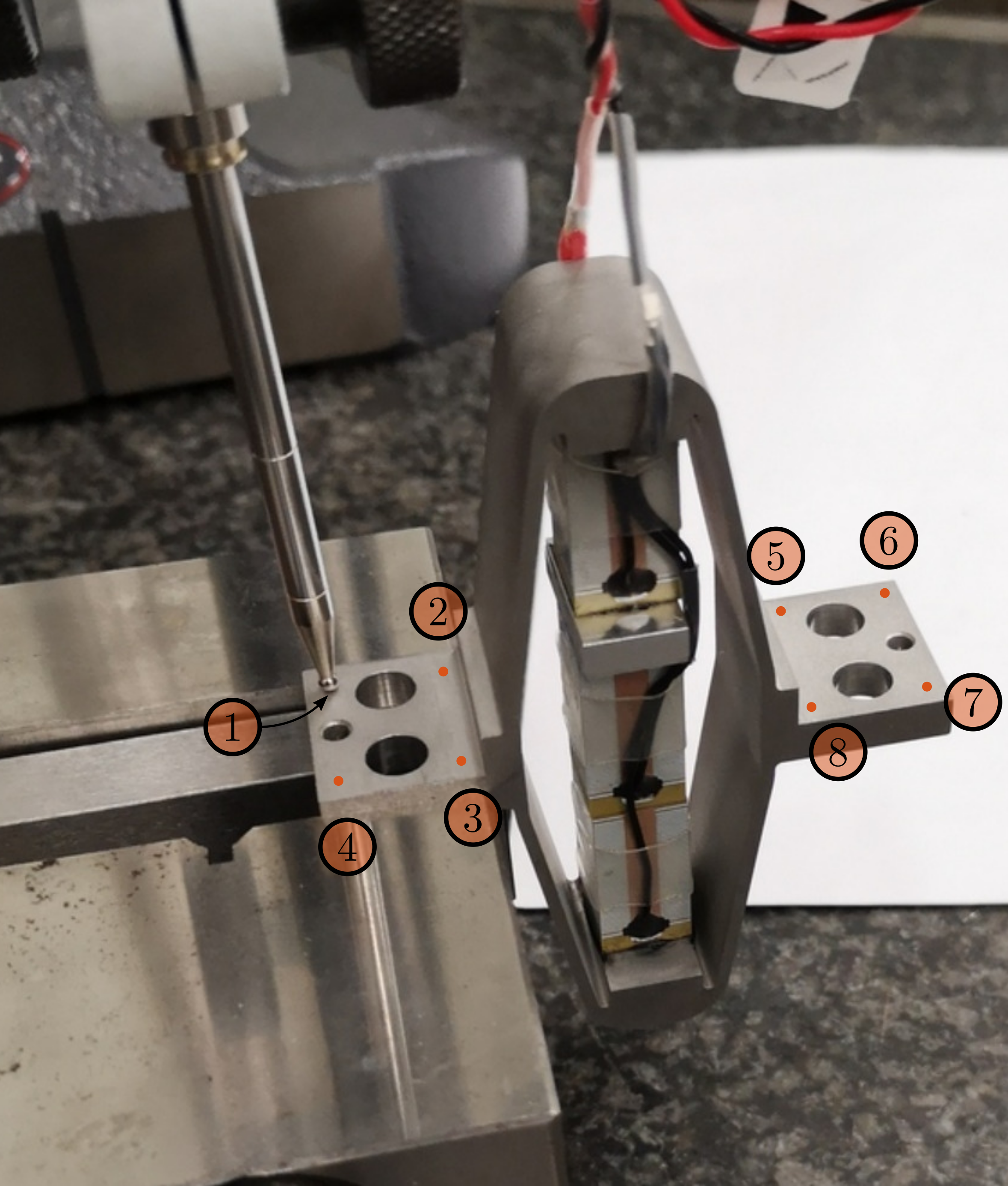
To measure the flatness of the two mechanical interfaces of the APA300ML, a small measurement bench is installed on top of a metrology granite with very good flatness.

As shown in Figure ref:fig:test_apa_flatness_setup, the APA is fixed to a clamp while a measuring probe¹ is used to measure the height of 4 points on each of the APA300ML interfaces.

From the X-Y-Z coordinates of the measured 8 points, the flatness is estimated by best fitting² a plane through all the points.

Measurement setup for flatness estimation of the two mechanical interfaces

%% Measured height for all the APA at the 8 locations
apa1 = 1e-6*[0, -0.5 , 3.5  , 3.5  , 42   , 45.5, 52.5 , 46];
apa2 = 1e-6*[0, -2.5 , -3   , 0    , -1.5 , 1   , -2   , -4];
apa3 = 1e-6*[0, -1.5 , 15   , 17.5 , 6.5  , 6.5 , 21   , 23];
apa4 = 1e-6*[0, 6.5  , 14.5 , 9    , 16   , 22  , 29.5 , 21];
apa5 = 1e-6*[0, -12.5, 16.5 , 28.5 , -43  , -52 , -22.5, -13.5];
apa6 = 1e-6*[0, -8   , -2   , 5    , -57.5, -62 , -55.5, -52.5];
apa7 = 1e-6*[0, 9    , -18.5, -30  , 31   , 46.5, 16.5 , 7.5];

apa = {apa1, apa2, apa3, apa4, apa5, apa6, apa7};

%% X-Y positions of the measurements points
W = 20e-3;   % Width [m]
L = 61e-3;   % Length [m]
d = 1e-3;    % Distance from border [m]
l = 15.5e-3; % [m]

pos = [[-L/2 + d,      W/2 - d];
       [-L/2 + l - d,  W/2 - d];
       [-L/2 + l - d, -W/2 + d];
       [-L/2 + d,     -W/2 + d];
       [L/2 - l + d,   W/2 - d];
       [L/2 - d,       W/2 - d];
       [L/2 - d,      -W/2 + d];
       [L/2 - l + d,  -W/2 + d]]';

%% Using fminsearch to find the best fitting plane
apa_d = zeros(1, 7); % Measured flatness of the APA
for i = 1:7
    fun = @(x)max(abs(([pos; apa{i}]-[0;0;x(1)])'*([x(2:3);1]/norm([x(2:3);1]))));
    x0 = [0;0;0];
    [x, min_d] = fminsearch(fun,x0);
    apa_d(i) = min_d;
end

The measured flatness, summarized in Table ref:tab:test_apa_flatness_meas, are within the specifications.

	Flatness $[\mu m]$
APA 1	8.9
APA 2	3.1
APA 3	9.1
APA 4	3.0
APA 5	1.9
APA 6	7.1
APA 7	18.7

Electrical Measurements

<<ssec:test_apa_electrical_measurements>>

From the documentation of the APA300ML, the total capacitance of the three stacks should be between $18\,\mu F$ and $26\,\mu F$ with a nominal capacitance of $20\,\mu F$.

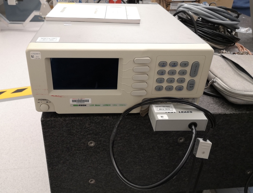
The capacitance of the piezoelectric stacks found in the APA300ML have been measured with the LCR meter³ shown in Figure ref:fig:test_apa_lcr_meter. The two stacks used as an actuator and the stack used as a force sensor are measured separately.

The measured capacitance are summarized in Table ref:tab:test_apa_capacitance and the average capacitance of one stack is $\approx 5 \mu F$. However, the measured capacitance of the stacks of "APA 3" is only half of the expected capacitance. This may indicate a manufacturing defect.

The measured capacitance is found to be lower than the specified one. This may be due to the fact that the manufacturer measures the capacitance with large signals ($-20\,V$ to $150\,V$) while it was here measured with small signals.

	Sensor Stack	Actuator Stacks
APA 1	5.10	10.03
APA 2	4.99	9.85
APA 3	1.72	5.18
APA 4	4.94	9.82
APA 5	4.90	9.66
APA 6	4.99	9.91
APA 7	4.85	9.85

Stroke and Hysteresis Measurement

<<ssec:test_apa_stroke_measurements>>

The goal is here to verify that the stroke of the APA300ML is as specified in the datasheet. To do so, one side of the APA is fixed to the granite, and a displacement probe⁴ is located on the other side as shown in Figure ref:fig:test_apa_stroke_bench.

Then, the voltage across the two actuator stacks is varied from $-20\,V$ to $150\,V$ using a DAC and a voltage amplifier. Note that the voltage is here slowly varied as the displacement probe has a very low measurement bandwidth (see Figure ref:fig:test_apa_stroke_bench, left).

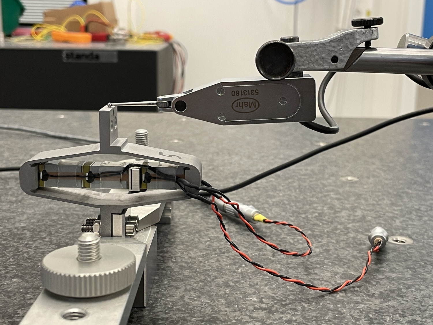
The measured APA displacement is shown as a function of the applied voltage in Figure ref:fig:test_apa_stroke_result, right.

Typical hysteresis curves for piezoelectric stack actuators can be observed. The measured stroke is approximately $250\,\mu m$ when using only two of the three stacks, which is enough for the current application. This is even above what is specified as the nominal stroke in the data-sheet ($304\,\mu m$, therefore $\approx 200\,\mu m$ if only two stacks are used).

It is clear from Figure ref:fig:test_apa_stroke_result that "APA 3" has an issue compared to the other units. This confirms the abnormal electrical measurements made in Section ref:ssec:test_apa_electrical_measurements. This unit was send sent back to Cedrat and a new one was shipped back. From now on, only the six APA that behave as expected will be used.

%% Load the measured strokes
load('meas_apa_stroke.mat', 'apa300ml_2s')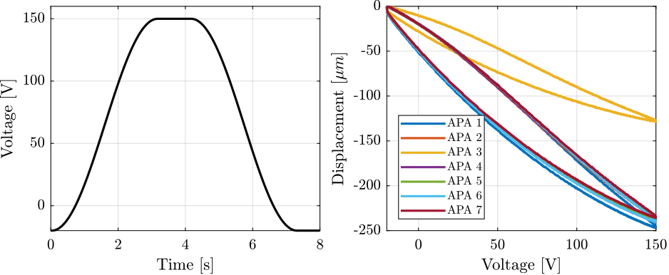

Generated voltage across the two piezoelectric stack actuators to estimate the stroke of the APA300ML (left). Measured displacement as a function of the applied voltage (right)

Flexible Mode Measurement

<<ssec:test_apa_spurious_resonances>>

In this section, the flexible modes of the APA300ML are investigated both experimentally and using a Finite Element Model.

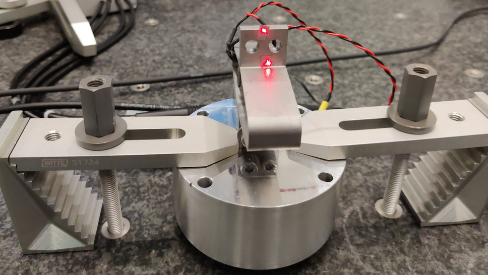
To experimentally estimate these modes, the APA is fixed on one end (see Figure ref:fig:test_apa_meas_setup_torsion). A Laser Doppler Vibrometer⁵ is used to measure the difference of motion between two "red" points (i.e. the torsion of the APA along the vertical direction) and an instrumented hammer⁶ is used to excite the flexible modes. Using this setup, the transfer function from the injected force to the measured rotation can be computed in different conditions and the frequency and mode shapes of the flexible modes can be estimated.

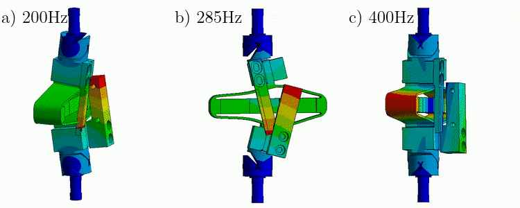
The flexible modes for the same condition (i.e. one mechanical interface of the APA300ML fixed) are estimated using a finite element software and the results are shown in Figure ref:fig:test_apa_mode_shapes.

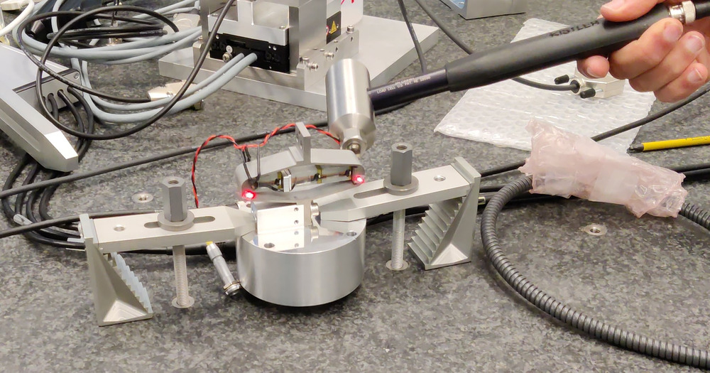
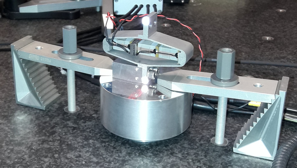
Two other similar measurements are performed to measured the bending of the APA around the $X$ direction and around the $Y$ direction (see Figure ref:fig:test_apa_meas_setup_modes).

Experimental setup to measured flexible modes of the APA300ML. For the bending in the $X$ direction, the impact point is located at the back of the top measurement point. For the bending in the $Y$ direction, the impact point is located on the back surface of the top interface (on the back of the 2 measurements points).

%% X-Bending Identification
% Load Data
bending_X = load('apa300ml_bending_X_top.mat');

% Spectral Analysis setup
Ts = bending_X.Track1_X_Resolution; % Sampling Time [s]
Nfft = floor(1/Ts);
win = hanning(Nfft);
Noverlap = floor(Nfft/2);

% Compute the transfer function from applied force to measured rotation
[G_bending_X, f]  = tfestimate(bending_X.Track1, bending_X.Track2, win, Noverlap, Nfft, 1/Ts);

%% Y-Bending identification
% Load Data
bending_Y = load('apa300ml_bending_Y_top.mat');

% Compute the transfer function
[G_bending_Y, ~]  = tfestimate(bending_Y.Track1, bending_Y.Track2, win, Noverlap, Nfft, 1/Ts);

%% Z-Torsion identification
% Load data
torsion = load('apa300ml_torsion_top.mat');

% Compute transfer function
[G_torsion_top, ~]  = tfestimate(torsion.Track1, torsion.Track2, win, Noverlap, Nfft, 1/Ts);

% Load Data
torsion = load('apa300ml_torsion_left.mat');

% Compute transfer function
[G_torsion, ~]  = tfestimate(torsion.Track1, torsion.Track2, win, Noverlap, Nfft, 1/Ts);

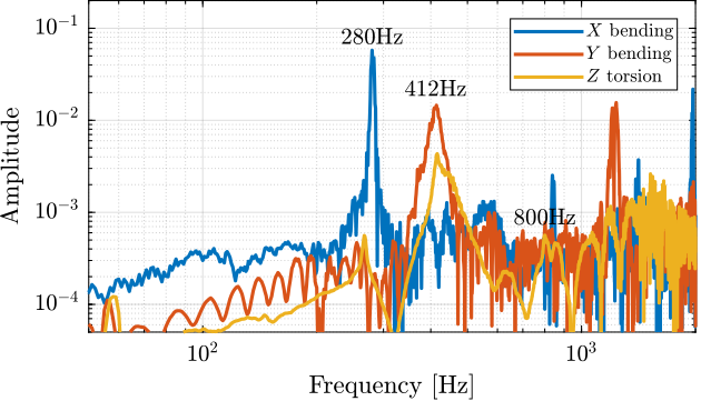
The three measured frequency response functions are shown in Figure ref:fig:test_apa_meas_freq_compare.

• a clear $x$ bending mode at $280\,\text{Hz}$
• a clear $y$ bending mode at $412\,\text{Hz}$
• for the $z$ torsion test, the $y$ bending mode is also excited and observed, and we may see a mode at $800\,\text{Hz}$

Obtained frequency response functions for the 3 tests with the instrumented hammer

Mode	FEM	Measured Frequency
$X$ bending		280Hz
$Y$ bending		410Hz
$Z$ torsion		800Hz

Conclusion   ignore

Dynamical measurements

<<sec:test_apa_dynamics>>

Introduction   ignore

After the basic measurements on the APA were performed in Section ref:sec:test_apa_basic_meas, a new test bench is used to better characterize the APA.

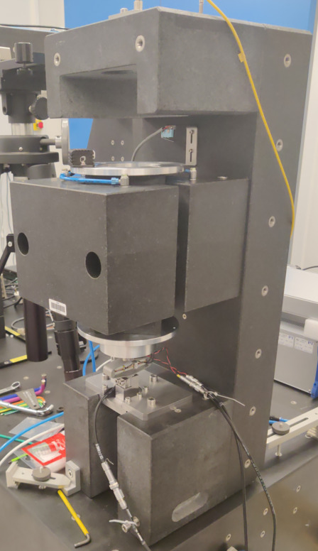
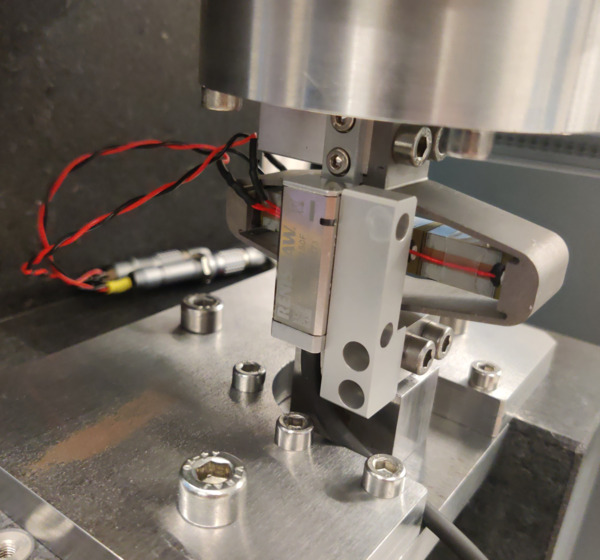
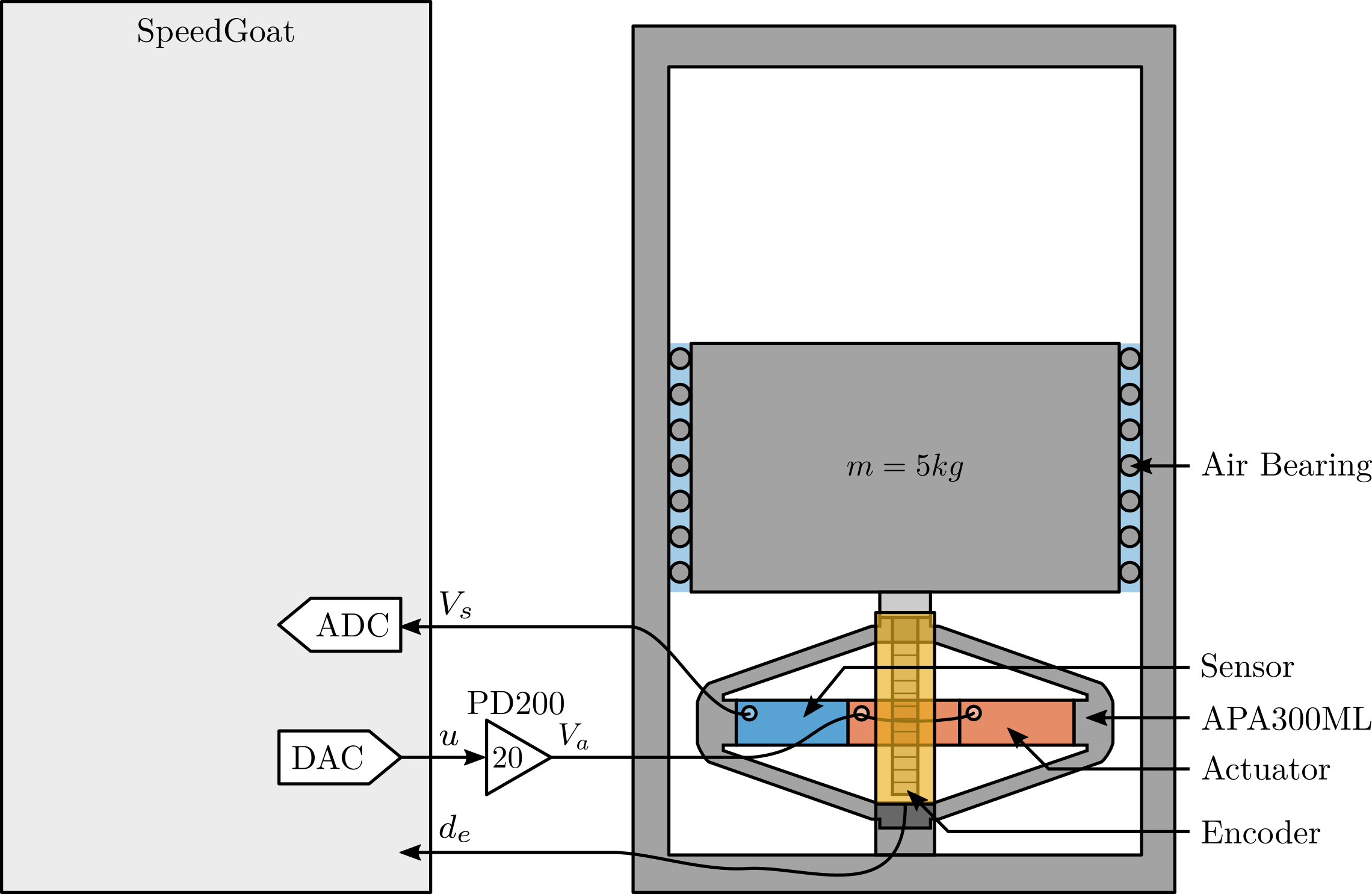
This test bench is shown in Figure ref:fig:test_bench_apa and consists of the APA300ML fixed on one end to the fixed granite, and on the other end to the 5kg granite vertically guided with an air bearing. An encoder is used to measure the relative motion between the two granites (i.e. the displacement of the APA).

Test bench used to characterize the APA300ML

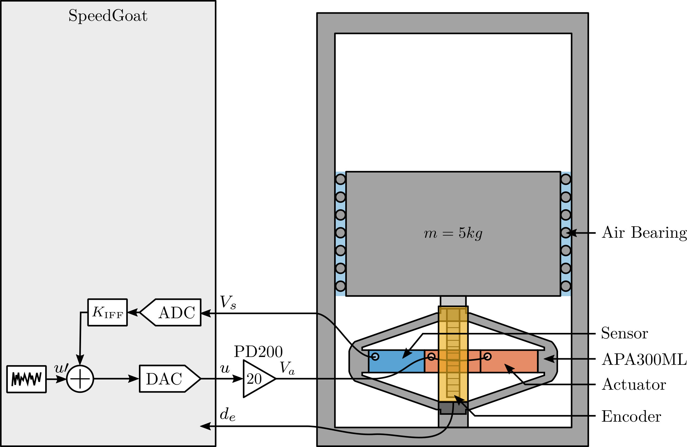
The bench is schematically shown in Figure ref:fig:test_apa_schematic and the signal used are summarized in Table ref:tab:test_apa_variables.

Variable	Description	Unit
$u$	Output DAC Voltage	$V$
$V_a$	Output Amplifier Voltage	$V$
$V_s$	Measured Stack Voltage (ADC)	$V$
$d_e$	Encoder Measurement	$m$

This bench will be used to:

• ref:ssec:test_apa_hysteresis
• ref:ssec:test_apa_stiffness
• measure the dynamics of the APA (section ref:ssec:test_apa_meas_dynamics)
• estimate the added damping using Integral Force Feedback (Section ref:ssec:test_apa_iff_locus)

These measurements will also be used to tune the developed models of the APA (in Section ref:sec:test_apa_model_2dof for the 2DoF model, and in Section ref:sec:test_apa_model_flexible for the flexible model).

Hysteresis

<<ssec:test_apa_hysteresis>>

As the payload is vertically guided without friction, the hysteresis of the APA can be estimated from the motion of the payload.

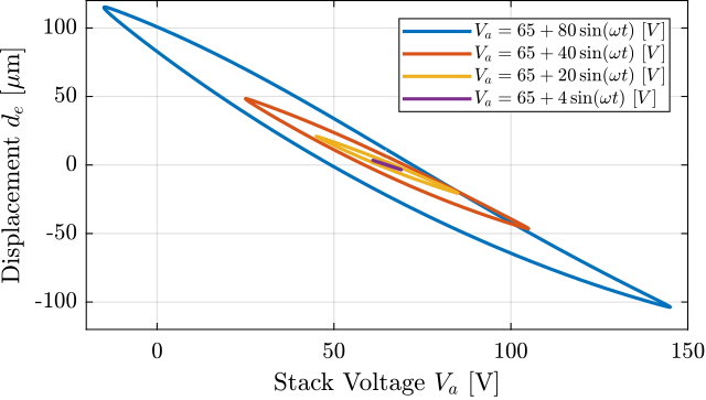
A quasi static sinusoidal excitation $V_a$ with an offset of $65\,V$ (halfway between $-20\,V$ and $150\,V$), and an amplitude varying from $4\,V$ up to $80\,V$.

For each excitation amplitude, the vertical displacement $d_e$ of the mass is measured and displayed as a function of the applied voltage..

%% Load measured data - hysteresis
apa_hyst = load('frf_data_1_hysteresis.mat', 't', 'u', 'de');

% Initial time set to zero
apa_hyst.t = apa_hyst.t - apa_hyst.t(1);

ampls = [0.1, 0.2, 0.4, 1, 2, 4]; % Excitation voltage amplitudes

The measured displacements as a function of the output voltages are shown in Figure ref:fig:test_apa_meas_hysteresis. It is interesting to see that the hysteresis is increasing with the excitation amplitude.

Obtained hysteresis curves (displacement as a function of applied voltage) for multiple excitation amplitudes

Axial stiffness

<<ssec:test_apa_stiffness>>

In order to estimate the stiffness of the APA, a weight with known mass $m_a = 6.4\,\text{kg}$ is added on top of the suspended granite and the deflection $d_e$ is measured using the encoder.

The APA stiffness can then be estimated from equation eqref:eq:test_apa_stiffness.

\begin{equation} \label{eq:test_apa_stiffness} k_{\text{apa}} = \frac{m_a g}{Δ d_e}

\end{equation}

%% Load data for stiffness measurement
apa_nums = [1 2 4 5 6 8];
apa_mass = {};
for i = 1:length(apa_nums)
    apa_mass(i) = {load(sprintf('frf_data_%i_add_mass_closed_circuit.mat', apa_nums(i)), 't', 'de')};
    % The initial displacement is set to zero
    apa_mass{i}.de = apa_mass{i}.de - mean(apa_mass{i}.de(apa_mass{i}.t<11));
end

added_mass = 6.4; % Added mass [kg]

The measured displacement $d_e$ as a function of time is shown in Figure ref:fig:test_apa_meas_stiffness_time. It can be seen that there are some drifts in the measured displacement (probably due to piezoelectric creep) and the that displacement does not come back to the initial position after the mass is removed (probably due to piezoelectric hysteresis). These two effects induce some uncertainties in the measured stiffness.

Measured displacement when adding the mass (at $t \approx 3\,s$) and removing the mass(at $t \approx 13\,s$)

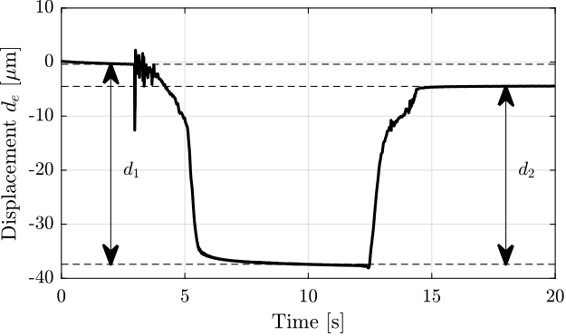
The stiffnesses are computed for all the APA from the two displacements $d_1$ and $d_2$ (see Figure ref:fig:test_apa_meas_stiffness_time) leading to two stiffness estimations $k_1$ and $k_2$. These estimated stiffnesses are summarized in Table ref:tab:test_apa_measured_stiffnesses and are found to be close to the nominal stiffness $k = 1.8\,N/\mu m$ found in the APA300ML manual.

APA	$k_1$	$k_2$
1	1.68	1.9
2	1.69	1.9
4	1.7	1.91
5	1.7	1.93
6	1.7	1.92
8	1.73	1.98

The stiffness can also be computed using equation eqref:eq:test_apa_res_freq by knowing the main vertical resonance frequency $\omega_z \approx 95\,\text{Hz}$ (estimated by the dynamical measurements shown in section ref:ssec:test_apa_meas_dynamics) and the suspended mass $m_{\text{sus}} = 5.7\,\text{kg}$.

\begin{equation} \label{eq:test_apa_res_freq} ω_z = \sqrt{\frac{k}{m_{\text{sus}}}}

\end{equation}

The obtain stiffness is $k \approx 2\,N/\mu m$ which is close to the values found in the documentation and by the "static deflection" method.

However, changes in the electrical impedance connected to the piezoelectric stacks impacts the mechanical compliance (or stiffness) of the piezoelectric stack cite:&reza06_piezoel_trans_vibrat_contr_dampin chap. 2.

To estimate this effect, the stiffness of the APA if measured using the "static deflection" method in two cases:

• $k_{\text{os}}$: piezoelectric stacks left unconnected (or connect to the high impedance ADC)
• $k_{\text{sc}}$: piezoelectric stacks short circuited (or connected to the voltage amplifier with small output impedance)

The open-circuit stiffness is estimated at $k_{\text{oc}} \approx 2.3\,N/\mu m$ and the closed-circuit stiffness $k_{\text{sc}} \approx 1.7\,N/\mu m$.

%% Load Data
add_mass_oc = load('frf_data_1_add_mass_open_circuit.mat',   't', 'de');
add_mass_cc = load('frf_data_1_add_mass_closed_circuit.mat', 't', 'de');

%% Zero displacement at initial time
add_mass_oc.de = add_mass_oc.de - mean(add_mass_oc.de(add_mass_oc.t<11));
add_mass_cc.de = add_mass_cc.de - mean(add_mass_cc.de(add_mass_cc.t<11));

%% Estimation of the stiffness in Open Circuit and Closed-Circuit
apa_k_oc = 9.8 * added_mass / (mean(add_mass_oc.de(add_mass_oc.t > 12 & add_mass_oc.t < 12.5)) - mean(add_mass_oc.de(add_mass_oc.t > 20 & add_mass_oc.t < 20.5)));
apa_k_sc = 9.8 * added_mass / (mean(add_mass_cc.de(add_mass_cc.t > 12 & add_mass_cc.t < 12.5)) - mean(add_mass_cc.de(add_mass_cc.t > 20 & add_mass_cc.t < 20.5)));

Dynamics

<<ssec:test_apa_meas_dynamics>>

In this section, the dynamics of the system from the excitation voltage $u$ to encoder measured displacement $d_e$ and to the force sensor voltage $V_s$ is identified.

%% Identification using sweep sine (low frequency)
load('frf_data_sweep.mat');
load('frf_data_noise_hf.mat');

%% Sampling Frequency
Ts = 1e-4; % Sampling Time [s]
Fs = 1/Ts; % Sampling Frequency [Hz]

%% "Hanning" windows used for the spectral analysis:
Nfft = floor(2/Ts);
win = hanning(Nfft);
Noverlap = floor(Nfft/2);

%% Separation of frequencies: low freqs using sweep sine, and high freq using noise
% Only used to have the frequency vector "f"
[~, f] = tfestimate(apa_sweep{1}.u, apa_sweep{1}.de, win, Noverlap, Nfft, 1/Ts);
i_lf = f <= 350;
i_hf = f >  350;

%% FRF estimation of the transfer function from u to de
enc_frf = zeros(length(f), length(apa_nums));
for i = 1:length(apa_nums)
    [frf_lf, ~] = tfestimate(apa_sweep{i}.u,    apa_sweep{i}.de,    win, Noverlap, Nfft, 1/Ts);
    [frf_hf, ~] = tfestimate(apa_noise_hf{i}.u, apa_noise_hf{i}.de, win, Noverlap, Nfft, 1/Ts);
    enc_frf(:, i) = [frf_lf(i_lf); frf_hf(i_hf)];
end

%% FRF estimation of the transfer function from u to Vs
iff_frf = zeros(length(f), length(apa_nums));
for i = 1:length(apa_nums)
    [frf_lf, ~] = tfestimate(apa_sweep{i}.u,    apa_sweep{i}.Vs,    win, Noverlap, Nfft, 1/Ts);
    [frf_hf, ~] = tfestimate(apa_noise_hf{i}.u, apa_noise_hf{i}.Vs, win, Noverlap, Nfft, 1/Ts);
    iff_frf(:, i) = [frf_lf(i_lf); frf_hf(i_hf)];
end

%% Save the identified dynamics for further analysis
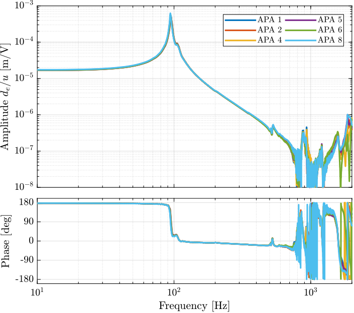
save('mat/meas_apa_frf.mat', 'f', 'Ts', 'enc_frf', 'iff_frf', 'apa_nums');

The obtained transfer functions for the 6 APA between the excitation voltage $u$ and the encoder displacement $d_e$ are shown in Figure ref:fig:test_apa_frf_encoder. The obtained transfer functions are close to a mass-spring-damper system. The following can be observed:

• A "stiffness line" indicating a static gain equal to $\approx -17\,\mu m/V$. The minus sign comes from the fact that an increase in voltage stretches the piezoelectric stack that then reduces the height of the APA
• A lightly damped resonance at $95\,\text{Hz}$
• A "mass line" up to $\approx 800\,\text{Hz}$, above which some resonances appear. These additional resonances might be coming from the limited stiffness of the encoder support or from the limited compliance of the APA support.

Estimated Frequency Response Function from generated voltage $u$ to the encoder displacement $d_e$ for the 6 APA300ML

The dynamics from $u$ to the measured voltage across the sensor stack $V_s$ is also identified and shown in Figure ref:fig:test_apa_frf_force.

A lightly damped resonance is observed at $95\,\text{Hz}$ and a lightly damped anti-resonance at $41\,\text{Hz}$. No additional resonances is present up to at least $2\,\text{kHz}$ indicating at Integral Force Feedback can be applied without stability issues from high frequency flexible modes.

As illustrated by the Root Locus, the poles of the closed-loop system converges to the zeros of the open-loop plant. Suppose that a controller with a very high gain is implemented such that the voltage $V_s$ across the sensor stack is zero. In that case, because of the very high controller gain, no stress and strain is present on the sensor stack (and on the actuator stacks are well, as they are both in series). Such closed-loop system would therefore virtually corresponds to a system for which the piezoelectric stacks have been removed and just the mechanical shell is kept. From this analysis, the axial stiffness of the shell can be estimated to be $k_{\text{shell}} = 5.7 \cdot (2\pi \cdot 41)^2 = 0.38\,N/\mu m$.

Such reasoning can lead to very interesting insight into the system just from an open-loop identification.

Estimated Frequency Response Function from generated voltage $u$ to the sensor stack voltage $V_s$ for the 6 APA300ML

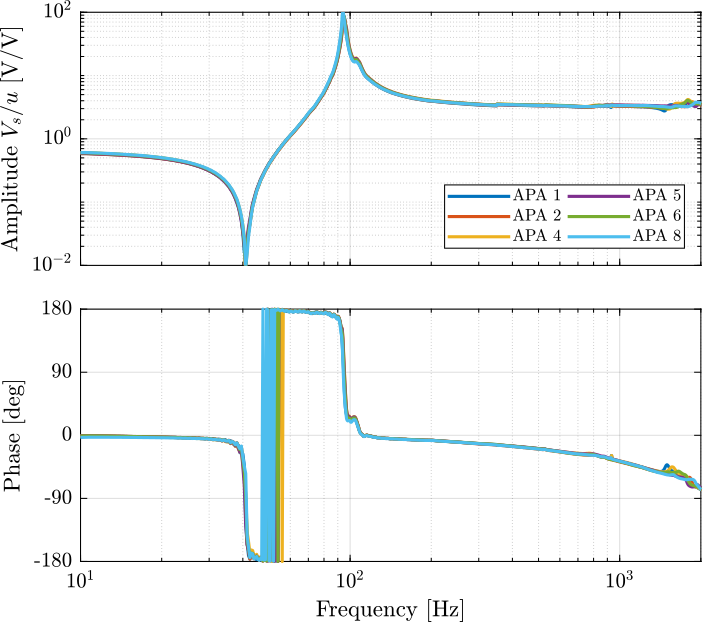
All the identified dynamics of the six APA300ML (both when looking at the encoder in Figure ref:fig:test_apa_frf_encoder and at the force sensor in Figure ref:fig:test_apa_frf_force) are almost identical, indicating good manufacturing repeatability for the piezoelectric stacks and the mechanical lever.

Effect of the resistor on the IFF Plant

<<ssec:test_apa_resistance_sensor_stack>>

A resistor $R \approx 80.6\,k\Omega$ is added in parallel with the sensor stack which has the effect to form a high pass filter with the capacitance of the stack.

As explain before, this is done for two reasons:

1. Limit the voltage offset due to the input bias current of the ADC
2. Limit the low frequency gain

The (low frequency) transfer function from $u$ to $V_s$ with and without this resistor have been measured and are compared in Figure ref:fig:test_apa_effect_resistance. It is confirmed that the added resistor as the effect of adding an high pass filter with a cut-off frequency of $\approx 0.35\,\text{Hz}$.

%% Load the data
wi_k = load('frf_data_1_sweep_lf_with_R.mat', 't', 'Vs', 'u'); % With the resistor
wo_k = load('frf_data_1_sweep_lf.mat',        't', 'Vs', 'u'); % Without the resistor

%% Large Hanning window for good low frequency estimate
Nfft = floor(50/Ts);
win = hanning(Nfft);
Noverlap = floor(Nfft/2);

%% Compute the transfer functions from u to Vs
[frf_wo_k, f] = tfestimate(wo_k.u, wo_k.Vs, win, Noverlap, Nfft, 1/Ts);
[frf_wi_k, ~] = tfestimate(wi_k.u, wi_k.Vs, win, Noverlap, Nfft, 1/Ts);

%% Model for the high pass filter
C = 5.1e-6; % Sensor Stack capacitance [F]
R = 80.6e3; % Parallel Resistor [Ohm]

f0 = 1/(2*pi*R*C); % Crossover frequency of RC HPF [Hz]

G_hpf = 0.6*(s/2*pi*f0)/(1 + s/2*pi*f0);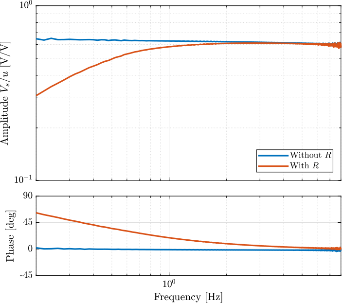

Transfer function from u to $V_s$ with and without the resistor $R$ in parallel with the piezoelectric stack used as the force sensor

Integral Force Feedback

<<ssec:test_apa_iff_locus>>

This test bench can also be used to estimate the damping added by the implementation of an Integral Force Feedback strategy.

%% Load identification Data
data = load("2023-03-17_11-28_iff_plant.mat");

%% Spectral Analysis setup
Ts = 1e-4; % Sampling Time [s]
Nfft = floor(5/Ts);
win = hanning(Nfft);
Noverlap = floor(Nfft/2);

%% Compute the transfer function from applied force to measured rotation
[G_iff, f]  = tfestimate(data.id_plant, data.Vs, win, Noverlap, Nfft, 1/Ts);

First, the transfer function eqref:eq:test_apa_iff_manual_fit is manually tuned to match the identified dynamics from generated voltage $u$ to the measured sensor stack voltage $V_s$ in Section ref:ssec:test_apa_meas_dynamics.

The obtained parameter values are $\omega_{\textsc{hpf}} = 0.4\, \text{Hz}$, $\omega_{z} = 42.7\, \text{Hz}$, $\xi_{z} = 0.4\,\%$, $\omega_{p} = 95.2\, \text{Hz}$, $\xi_{p} = 2\,\%$ and $g_0 = 0.64$.

\begin{equation} \label{eq:test_apa_iff_manual_fit} G_{\textsc{iff},m}(s) = g_0 ⋅ \frac{1 + 2 ξ_z \frac{s}{ω_z} + \frac{s^2}{ω_z^2}}{1 + 2 ξ_p \frac{s}{ω_p} + \frac{s^2}{ω_p^2}} ⋅ \frac{s}{ω_{\textsc{hpf}} + s}

\end{equation}

The comparison between the identified plant and the manually tuned transfer function is done in Figure ref:fig:test_apa_iff_plant_comp_manual_fit.

%% Basic manually tuned model
w0z = 2*pi*42.7; % Zero frequency
xiz = 0.004; % Zero damping

w0p = 2*pi*95.2; % Pole frequency
xip = 0.02; % Pole damping

G_iff_model = exp(-2*s*Ts)*0.64*(1 + 2*xiz/w0z*s + s^2/w0z^2)/(1 + 2*xip/w0p*s + s^2/w0p^2)*(s/(s+2*pi*0.4));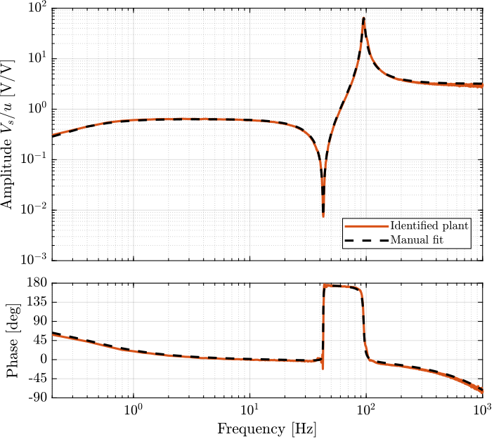

Identified IFF plant and manually tuned model of the plant (a time delay of $200\,\mu s$ is added to the model of the plant to better match the identified phase)

The implemented Integral Force Feedback Controller transfer function is shown in equation eqref:eq:test_apa_Kiff_formula. It contains an high pass filter (cut-off frequency of $2\,\text{Hz}$) to limit the low frequency gain, a low pass filter to add integral action above $20\,\text{Hz}$, a second low pass filter to add robustness to high frequency resonances and a tunable gain $g$.

\begin{equation} \label{eq:test_apa_Kiff_formula} K_{\textsc{iff}}(s) = -10 ⋅ g ⋅ \frac{s}{s + 2π ⋅ 2} ⋅ \frac{1}{1 + 2π ⋅ 20} ⋅ \frac{1}{s + 2π⋅ 2000}

\end{equation}

%% Integral Force Feedback Controller
K_iff = -10*(1/(s + 2*pi*20)) * ... % LPF: provides integral action above 20Hz
            (s/(s + 2*pi*2))  * ... % HPF: limit low frequency gain
            (1/(1 + s/2/pi/2e3));   % LPF: more robust to high frequency resonances

To estimate how the dynamics of the APA changes when the Integral Force Feedback controller is implemented, the test bench shown in Figure ref:fig:test_apa_iff_schematic is used. The transfer function from the "damped" plant input $u\prime$ to the encoder displacement $d_e$ is identified for several IFF controller gains $g$.

Figure caption

%% Load Data
data = load("2023-03-17_14-10_damped_plants_new.mat");

%% Spectral Analysis setup
Ts = 1e-4; % Sampling Time [s]
Nfft = floor(1/Ts);
win = hanning(Nfft);
Noverlap = floor(Nfft/2);

%% Get the frequency vector
[~, f]  = tfestimate(data.data(1).id_plant(1:end), data.data(1).dL(1:end), win, Noverlap, Nfft, 1/Ts);

%% Gains used for analysis are between 1 and 50
i_kept = [5:10];

%% Identify the damped plant from u' to de for different IFF gains
G_dL_frf = {zeros(1,length(i_kept))};

for i = 1:length(i_kept)
    [G_dL, ~]  = tfestimate(data.data(i_kept(i)).id_plant(1:end), data.data(i_kept(i)).dL(1:end), win, Noverlap, Nfft, 1/Ts);
    G_dL_frf(i) = {G_dL};
end

The identified dynamics are then fitted by second order transfer functions. The comparison between the identified damped dynamics and the fitted second order transfer functions is done in Figure ref:fig:test_apa_identified_damped_plants for different gains $g$. It is clear that large amount of damping is added when the gain is increased and that the frequency of the pole is shifted to lower frequencies.

%% Fit the data with 2nd order transfer function using vectfit3
opts = struct();

opts.stable = 1;    % Enforce stable poles
opts.asymp = 1;     % Force D matrix to be null
opts.relax = 1;     % Use vector fitting with relaxed non-triviality constraint
opts.skip_pole = 0; % Do NOT skip pole identification
opts.skip_res = 0;  % Do NOT skip identification of residues (C,D,E)
opts.cmplx_ss = 0;  % Create real state space model with block diagonal A

opts.spy1 = 0;      % No plotting for first stage of vector fitting
opts.spy2 = 0;      % Create magnitude plot for fitting of f(s)

Niter = 100; % Number of iteration.
N = 2; % Order of approximation
poles = [-25 - 1i*60, -25 + 1i*60]; % First get for the pole location

G_dL_id  = {zeros(1,length(i_kept))};

% Identification just between two frequencies
f_keep = (f>5 & f<200);

for i = 1:length(i_kept)
    %% Estimate resonance frequency and damping
    for iter = 1:Niter
        [G_est, poles, ~, frf_est] = vectfit3(G_dL_frf{i}(f_keep).', 1i*2*pi*f(f_keep)', poles, ones(size(f(f_keep)))', opts);
    end
    G_dL_id(i) = {ss(G_est.A, G_est.B, G_est.C, G_est.D)};
end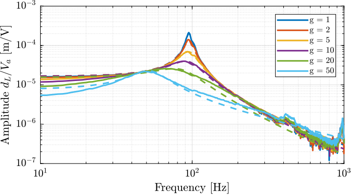

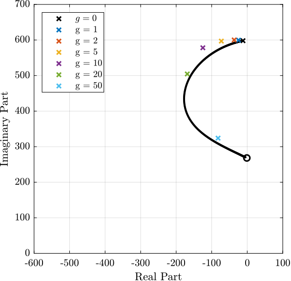
Identified dynamics (solid lines) and fitted transfer functions (dashed lines) from $u\prime$ to $d_e$ for different IFF gains

The evolution of the pole in the complex plane as a function of the controller gain $g$ (i.e. the "root locus") is computed:

• using the IFF plant model eqref:eq:test_apa_iff_manual_fit and the implemented controller eqref:eq:test_apa_Kiff_formula
• from the fitted transfer functions of the damped plants experimentally identified for several controller gains

The two obtained root loci are compared in Figure ref:fig:test_apa_iff_root_locus and are in good agreement considering that the damped plants were only fitted using a second order transfer function.

Root Locus of the APA300ML with Integral Force Feedback - Comparison between the computed root locus from the plant model (black line) and the root locus estimated from the damped plant pole identification (colorful crosses)

Conclusion   ignore

So far, all the measured FRF are showing the dynamical behavior that was expected.

APA300ML - 2 Degrees of Freedom Model

<<sec:test_apa_model_2dof>>

Introduction   ignore

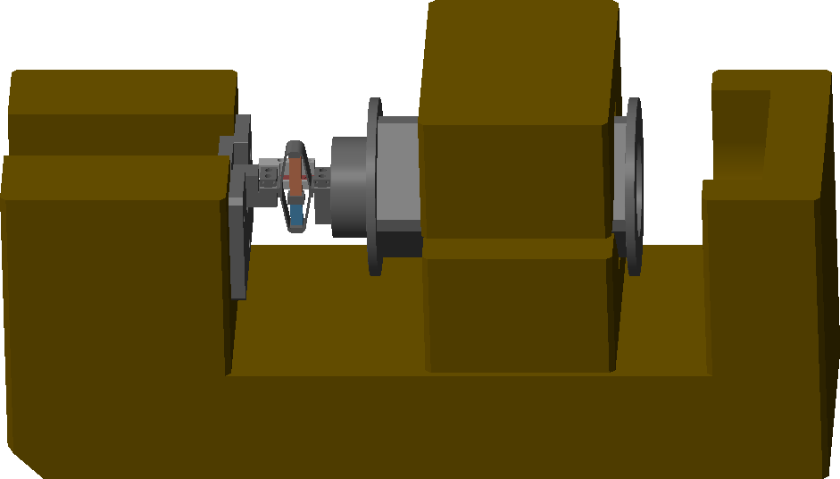
In this section, a simscape model (Figure ref:fig:test_apa_bench_model) of the measurement bench is used to compare the model of the APA with the measured frequency response functions.

A 2 degrees of freedom model is used to model the APA300ML. This model is presented in Section ref:ssec:test_apa_2dof_model and the procedure to tuned the model is described in Section ref:ssec:test_apa_2dof_model_tuning. The obtained model dynamics is compared with the measurements in Section ref:ssec:test_apa_2dof_model_result.

Two Degrees of Freedom APA Model

<<ssec:test_apa_2dof_model>>

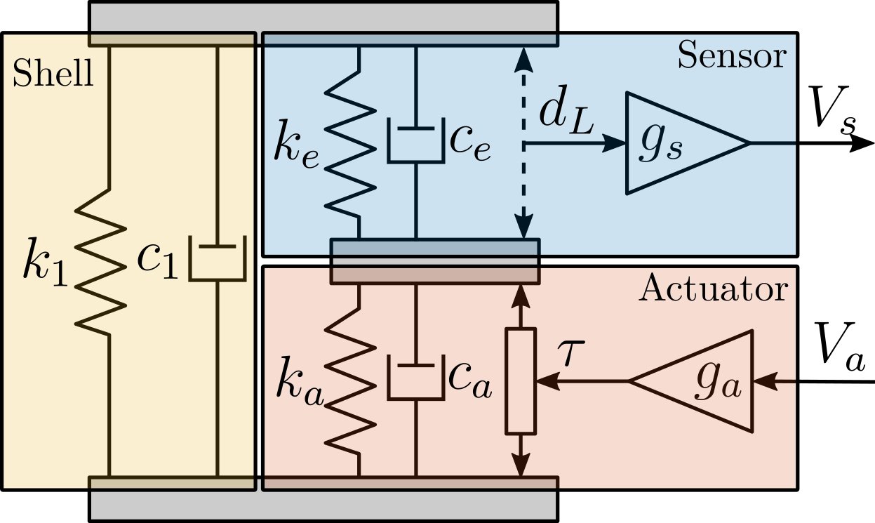
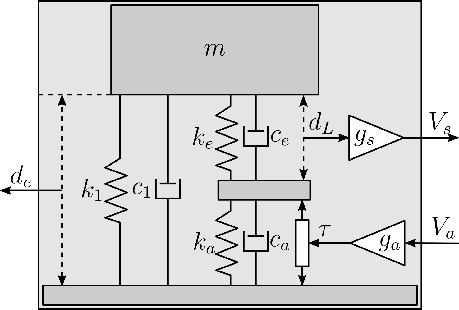
The APA model shown in Figure ref:fig:test_apa_2dof_model is adapted from cite:souleille18_concep_activ_mount_space_applic.

It can be decomposed into three components:

• the shell whose axial properties are represented by $k_1$ and $c_1$
• the actuator stacks whose contribution in the axial stiffness is represented by $k_a$ and $c_a$. A force source $\tau$ represents the axial force induced by the force sensor stacks. The gain $g_a$ (in $N/m$) is used to convert the applied voltage $V_a$ to the axial force $\tau$
• the actuator stacks whose contribution in the axial stiffness is represented by $k_e$ and $c_e$. A "strain sensor" $d_L$, and a gain $g_s$ (in $V/m$) that converts this strain into a generated voltage

Such simple model has some limitations:

• it only represents the axial characteristics of the APA (infinitely rigid in other directions)
• some physical insights are lost such as the amplification factor, the real stress and strain on the piezoelectric stacks
• it is fully linear and therefore the creep and hysteresis of the piezoelectric stacks are not modelled

Schematic of the two degrees of freedom model of the APA300ML

Tuning of the APA model

<<ssec:test_apa_2dof_model_tuning>>

9 parameters ($m$, $k_1$, $c_1$, $k_e$, $c_e$, $k_a$, $c_a$, $g_s$ and $g_a$) have to be tuned such that the dynamics of the model (Figure ref:fig:test_apa_2dof_model_simscape) well represents the identified dynamics in Section ref:sec:test_apa_dynamics.

Schematic of the two degrees of freedom model of the APA300ML with input $V_a$ and outputs $d_e$ and $V_s$

%% Stiffness values for the 2DoF APA model
k1 = 0.38e6; % Estimated Shell Stiffness [N/m]

w0 = 2*pi*95; % Resonance frequency [rad/s]
m = 5.7; % Suspended mass [kg]
ktot = m*(w0)^2; % Total Axial Stiffness to have to wanted resonance frequency [N/m]

ka = 1.5*(ktot-k1); % Stiffness of the (two) actuator stacks [N/m]
ke = 2*ka; % Stiffness of the Sensor stack [N/m]

%% Damping values for the 2DoF APA model
c1 = 20;   % Damping for the Shell [N/(m/s)]
ca = 100;  % Damping of the actuators stacks [N/(m/s)]
ce = 2*ca; % Damping of the sensor stack [N/(m/s)]

%% Estimation ot the sensor and actuator gains
% Initialize the structure with unitary sensor and actuator "gains"
n_hexapod = struct();
n_hexapod.actuator = initializeAPA(...
    'type', '2dof', ...
    'k',  k1,  ...
    'ka', ka,  ...
    'ke', ke,  ...
    'c',  c1, ...
    'ca', ca, ...
    'ce', ce, ...
    'Ga', 1,   ... % Actuator constant [N/V]
    'Gs', 1    ... % Sensor constant [V/m]
);

c_granite = 0; % Do not take into account damping added by the air bearing

% Run the linearization
G_norm = linearize(mdl, io, 0.0, opts);
G_norm.InputName  = {'u'};
G_norm.OutputName = {'Vs', 'de'};

% Load Identification Data to estimate the two gains
load('meas_apa_frf.mat', 'f', 'Ts', 'enc_frf', 'iff_frf', 'apa_nums');

% Estimation ot the Actuator Gain
fa = 10; % Frequency where the two FRF should match [Hz]
[~, i_f] = min(abs(f - fa));
ga = -abs(enc_frf(i_f,1))./abs(evalfr(G_norm('de', 'u'), 1i*2*pi*fa));

% Estimation ot the Sensor Gain
fs = 600; % Frequency where the two FRF should match [Hz]
[~, i_f] = min(abs(f - fs));
gs = -abs(iff_frf(i_f,1))./abs(evalfr(G_norm('Vs', 'u'), 1i*2*pi*fs))/ga;

First, the mass supported by the APA300ML can simply be estimated from the geometry and density of the different parts or by directly measuring it using a precise weighing scale. Both methods leads to an estimated mass of $5.7\,\text{kg}$.

Then, the axial stiffness of the shell was estimated at $k_1 = 0.38\,N/\mu m$ in Section ref:ssec:test_apa_meas_dynamics from the frequency of the anti-resonance seen on Figure ref:fig:test_apa_frf_force. Similarly, $c_1$ can be estimated from the damping ratio of the same anti-resonance and is found to be close to $20\,Ns/m$.

Then, it is reasonable to make the assumption that the sensor stacks and the two actuator stacks have identical mechanical characteristics⁷. Therefore, we have $k_e = 2 k_a$ and $c_e = 2 c_a$ as the actuator stack is composed of two stacks in series. In that case, the total stiffness of the APA model is described by eqref:eq:test_apa_2dof_stiffness.

\begin{equation}\label{eq:test_apa_2dof_stiffness} k_{\text{tot}} = k_1 + \frac{k_e k_a}{k_e + k_a} = k_1 + \frac{2}{3} k_a

\end{equation}

Knowing from eqref:eq:test_apa_tot_stiffness that the total stiffness is $k_{\text{tot}} = 2\,N/\mu m$, we get from eqref:eq:test_apa_2dof_stiffness that $k_a = 2.5\,N/\mu m$ and $k_e = 5\,N/\mu m$.

\begin{equation}\label{eq:test_apa_tot_stiffness} ω_0 = \frac{k_{\text{tot}}}{m} \Longrightarrow k_{\text{tot}} = m ω_0^2 = 2\,N/μ m \quad \text{with}\ m = 5.7\,\text{kg}\ \text{and}\ ω_0 = 2π ⋅ 95\, \text{rad}/s

\end{equation}

Then, $c_a$ (and therefore $c_e = 2 c_a$) can be tuned to match the damping ratio of the identified resonance. $c_a = 100\,Ns/m$ and $c_e = 200\,Ns/m$ are obtained.

Finally, the two gains $g_s$ and $g_a$ can be used to match the gain of the identified transfer functions.

The obtained parameters of the model shown in Figure ref:fig:test_apa_2dof_model_simscape are summarized in Table ref:tab:test_apa_2dof_parameters.

Parameter	Value
$m$	$5.7\,\text{kg}$
$k_1$	$0.38\,N/\mu m$
$k_e$	$5.0\, N/\mu m$
$k_a$	$2.5\,N/\mu m$
$c_1$	$20\,Ns/m$
$c_e$	$200\,Ns/m$
$c_a$	$100\,Ns/m$
$g_a$	$-2.58\,N/V$
$g_s$	$0.46\,V/\mu m$

Obtained Dynamics

<<ssec:test_apa_2dof_model_result>>

The dynamics of the 2DoF APA300ML model is now extracted using optimized parameters (listed in Table ref:tab:test_apa_2dof_parameters) from the Simscape model. It is compared with the experimental data in Figure ref:fig:test_apa_2dof_comp_frf.

A good match can be observed between the model and the experimental data, both for the encoder and for the force sensor. This indicates that this model represents well the axial dynamics of the APA300ML.

%% 2DoF APA300ML with optimized parameters
n_hexapod = struct();
n_hexapod.actuator = initializeAPA( ...
    'type', '2dof', ...
    'k',  k1,  ...
    'ka', ka,  ...
    'ke', ke,  ...
    'c',  c1, ...
    'ca', ca, ...
    'ce', ce, ...
    'Ga', ga, ...
    'Gs', gs  ...
);

%% Identification of the APA300ML with optimized parameters
G_2dof = exp(-s*Ts)*linearize(mdl, io, 0.0, opts);
G_2dof.InputName  = {'u'};
G_2dof.OutputName = {'Vs', 'de'};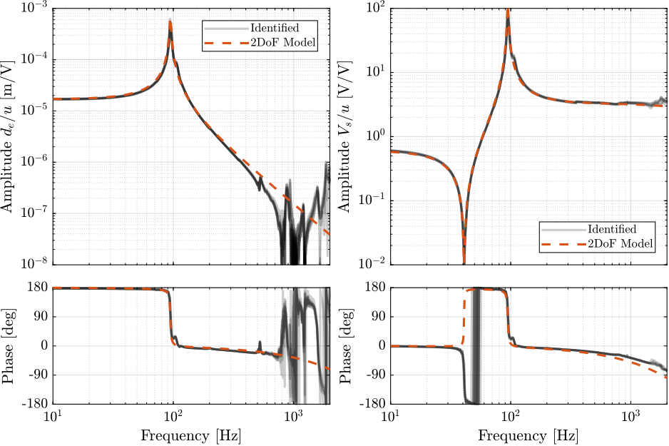

Comparison of the measured FRF and the optimized 2DoF model of the APA300ML

Conclusion   ignore

APA300ML - Super Element

<<sec:test_apa_model_flexible>>

Introduction   ignore

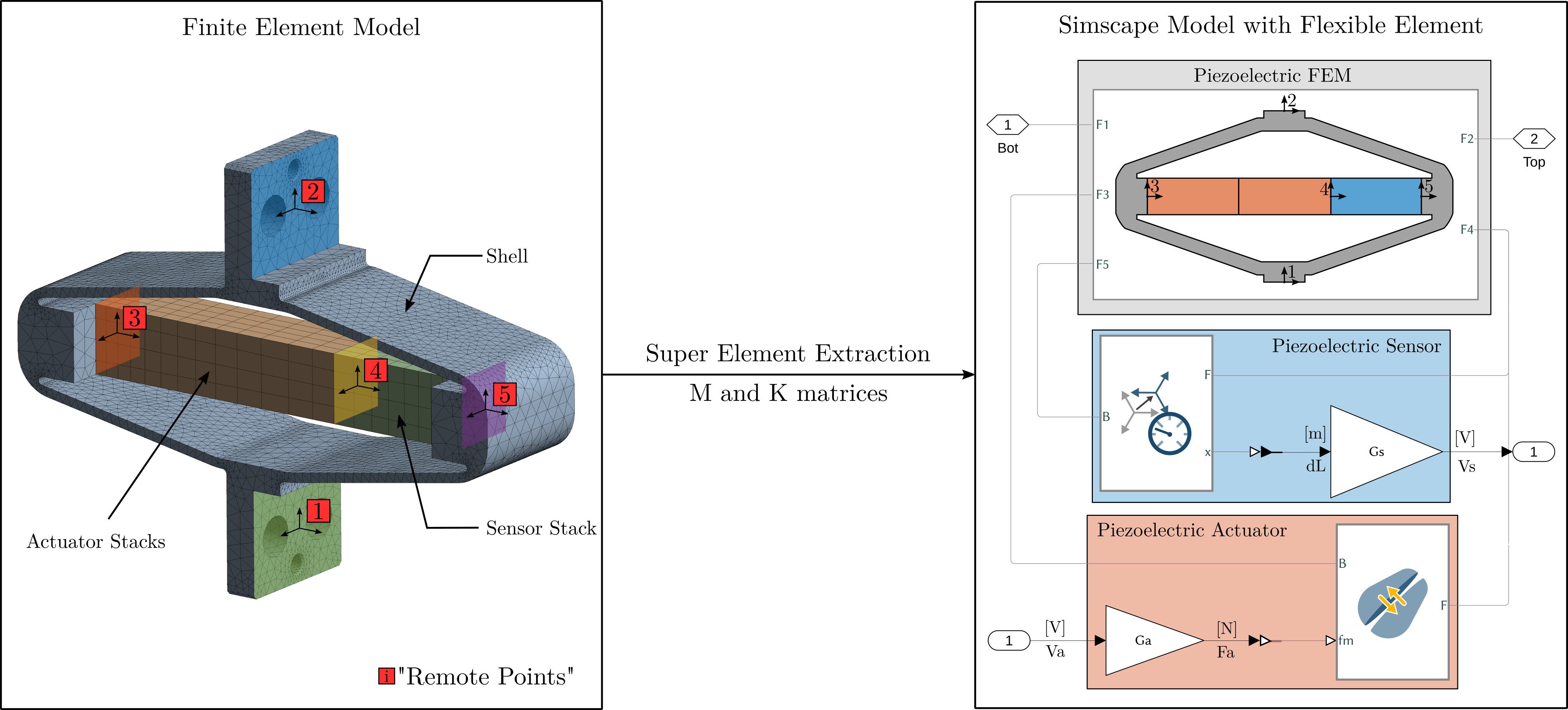
In this section, a super element of the Amplified Piezoelectric Actuator "APA300ML" is extracted using a Finite Element Software. It is then imported in Simscape (using the stiffness and mass matrices) and it is included in the same model that was used in ref:sec:test_apa_model_2dof.

This procedure is illustrated in Figure ref:fig:test_apa_super_element_simscape.

Extraction of the super-element

• Explain how the "remote points" are chosen
• Show some parts of the mass and stiffness matrices?
• Say which materials were used?
• Maybe this was already explain earlier in the manuscript

Identification of the Actuator and Sensor constants

<<ssec:test_apa_flexible_ga_gs>>

Once the APA300ML super element is included in the Simscape model, the transfer function from $F_a$ to $d_L$ and $d_e$ can be identified. The gains $g_a$ and $g_s$ can then be tuned such that the gain of the transfer functions are matching the identified ones.

By doing so, $g_s = 4.9\,V/\mu m$ and $g_a = 23.2\,N/V$ are obtained.

%% Identification of the actuator and sensor "constants"
% Initialize the APA as a flexible body with unity "constants"
n_hexapod.actuator = initializeAPA(...
    'type', 'flexible', ...
    'ga', 1, ...
    'gs', 1);

c_granite = 100; % Rought estimation of the damping added by the air bearing

% Identify the dynamics
G_norm = linearize(mdl, io, 0.0, opts);
G_norm.InputName  = {'u'};
G_norm.OutputName = {'Vs', 'de'};

% Load Identification Data to estimate the two gains
load('meas_apa_frf.mat', 'f', 'Ts', 'enc_frf', 'iff_frf', 'apa_nums');

% Actuator Constant in [N/V]
ga = -mean(abs(enc_frf(f>10 & f<20)))./dcgain(G_norm('de', 'u'));

% Sensor Constant in [V/m]
gs = -mean(abs(iff_frf(f>400 & f<500)))./(ga*abs(squeeze(freqresp(G_norm('Vs', 'u'), 1e3, 'Hz'))));

To make sure these "gains" are physically valid, it is possible to estimate them from physical properties of the piezoelectric stack material.

From cite:&fleming14_desig_model_contr_nanop_system p. 123, the relation between relative displacement $d_L$ of the sensor stack and generated voltage $V_s$ is given by eqref:eq:test_apa_piezo_strain_to_voltage and from cite:&fleming10_integ_strain_force_feedb_high the relation between the force $F_a$ and the applied voltage $V_a$ is given by eqref:eq:test_apa_piezo_voltage_to_force.

\begin{subequations} \begin{align} V_s &= \underbrace{\frac{d_{33}}{\epsilon^T s^D n}}_{g_s} d_L \label{eq:test_apa_piezo_strain_to_voltage} \\ F_a &= \underbrace{d_{33} n k_a}_{g_a} \cdot V_a, \quad k_a = \frac{c^{E} A}{L} \label{eq:test_apa_piezo_voltage_to_force} \end{align} \end{subequations}

Parameters used in equations eqref:eq:test_apa_piezo_strain_to_voltage and eqref:eq:test_apa_piezo_voltage_to_force are described in Table ref:tab:test_apa_piezo_properties.

Unfortunately, the manufacturer of the stack was not willing to share the piezoelectric material properties of the stack used in the APA300ML. However, based on available properties of the APA300ML stacks in the data-sheet, the soft Lead Zirconate Titanate "THP5H" from Thorlabs seemed to match quite well the observed properties. The properties of this "THP5H" material used to compute $g_a$ and $g_s$ are listed in Table ref:tab:test_apa_piezo_properties.

From these parameters, $g_s = 5.1\,V/\mu m$ and $g_a = 26\,N/V$ were obtained which are very close to the identified constants using the experimentally identified transfer functions.

Parameter	Value	Description
$d_{33}$	$680 \cdot 10^{-12}\,m/V$	Piezoelectric constant
$\epsilon^{T}$	$4.0 \cdot 10^{-8}\,F/m$	Permittivity under constant stress
$s^{D}$	$21 \cdot 10^{-12}\,m^2/N$	Elastic compliance understand constant electric displacement
$c^{E}$	$48 \cdot 10^{9}\,N/m^2$	Young's modulus of elasticity
$L$	$20\,mm$ per stack	Length of the stack
$A$	$10^{-4}\,m^2$	Area of the piezoelectric stack
$n$	$160$ per stack	Number of layers in the piezoelectric stack

%% Estimate "Sensor Constant" - (THP5H)
d33 = 680e-12;        % Strain constant [m/V]
n   = 160;            % Number of layers per stack
eT  = 4500*8.854e-12; % Permittivity under constant stress [F/m]
sD  = 21e-12;         % Compliance under constant electric displacement [m2/N]

gs_th = d33/(eT*sD*n);   % Sensor Constant [V/m]

%% Estimate "Actuator Constant" - (THP5H)
d33 = 680e-12;   % Strain constant [m/V]
n   = 320;       % Number of layers

cE  = 1/sD;      % Youngs modulus [N/m^2]
A   = (10e-3)^2; % Area of the stacks [m^2]
L   = 40e-3;     % Length of the two stacks [m]
ka  = cE*A/L;    % Stiffness of the two stacks [N/m]

ga_th = d33*n*ka;   % Actuator Constant [N/V]

Comparison of the obtained dynamics

<<ssec:test_apa_flexible_comp_frf>>

The obtained dynamics using the super element with the tuned "sensor gain" and "actuator gain" are compared with the experimentally identified frequency response functions in Figure ref:fig:test_apa_super_element_comp_frf.

A good match between the model and the experimental results is observed.

• the super element

This model represents fairly

The flexible model is a bit "soft" as compared with the experimental results.

This method can be used to model piezoelectric stack actuators as well as amplified piezoelectric stack actuators.

%% Idenfify the dynamics of the Simscape model with correct actuator and sensor "constants"
% Initialize the APA
n_hexapod.actuator = initializeAPA(...
    'type', 'flexible', ...
    'ga',   23.2, ... % Actuator gain [N/V]
    'gs',   -4.9e6);    % Sensor gain [V/m]

% Identify with updated constants
G_flex = exp(-Ts*s)*linearize(mdl, io, 0.0, opts);
G_flex.InputName  = {'u'};
G_flex.OutputName = {'Vs', 'de'};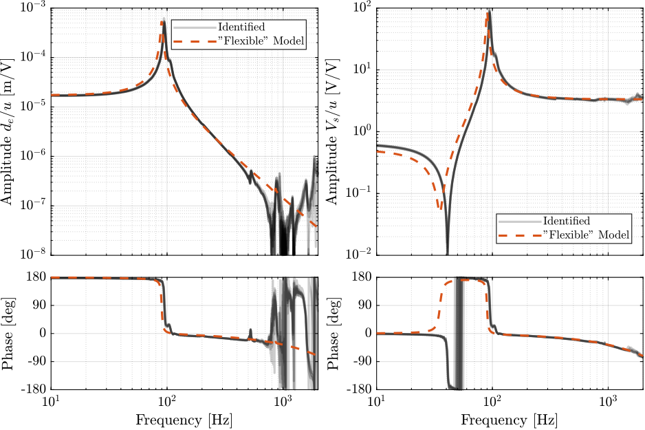

Comparison of the measured FRF and the "Flexible" model of the APA300ML

Conclusion   ignore

Conclusion

<<sec:test_apa_conclusion>>

• Compare 2DoF and FEM models (usefulness of the two)
• Good match between all the APA: will simplify the modeling and control of the nano-hexapod
• No advantage of the FEM model here (as only uniaxial behavior is checked), but may be useful later

Bibliography   ignore

Footnotes

⁶Kistler 9722A ⁵Polytec controller 3001 with sensor heads OFV512 ⁷Note that this is not fully correct as it was shown in Section ref:ssec:test_apa_stiffness that the electrical boundaries of the piezoelectric stack impacts its stiffness and that the sensor stack is almost open-circuited while the actuator stacks are almost short-circuited. ²The Matlab fminsearch command is used to fit the plane ¹Heidenhain MT25, specified accuracy of $0.5\,\mu m$ ⁴Millimar 1318 probe, specified linearity better than $1\,\mu m$ ³LCR-819 from Gwinstek, specified accuracy of $0.05\%$, measured frequency is set at $1\,\text{kHz}$

---