90 KiB
Test Bench - Amplified Piezoelectric Actuator
- Glossary and Acronyms - Tables
- Introduction
- First Basic Measurements
- Dynamical measurements
- APA300ML - 2 degrees-of-freedom Model
- APA300ML - Super Element
- Conclusion
- Bibliography
- Glossary
- Footnotes
This report is also available as a pdf.
Glossary and Acronyms - Tables ignore
| label | name | description |
|---|---|---|
| psdx | \ensuremath{Φx} | Power spectral density of signal $x$ |
| asdx | \ensuremath{Γx} | Amplitude spectral density of signal $x$ |
| cpsx | \ensuremath{Φx} | Cumulative Power Spectrum of signal $x$ |
| casx | \ensuremath{Γx} | Cumulative Amplitude Spectrum of signal $x$ |
| key | abbreviation | full form |
|---|---|---|
| haclac | HAC-LAC | High Authority Control - Low Authority Control |
| hac | HAC | High Authority Control |
| lac | LAC | Low Authority Control |
| nass | NASS | Nano Active Stabilization System |
| asd | ASD | Amplitude Spectral Density |
| psd | PSD | Power Spectral Density |
| cps | CPS | Cumulative Power Spectrum |
| cas | CAS | Cumulative Amplitude Spectrum |
| frf | FRF | Frequency Response Function |
| iff | IFF | Integral Force Feedback |
| rdc | RDC | Relative Damping Control |
| drga | DRGA | Dynamical Relative Gain Array |
| hpf | HPF | high-pass filter |
| lpf | LPF | low-pass filter |
| dof | DoF | degrees-of-freedom |
Introduction ignore
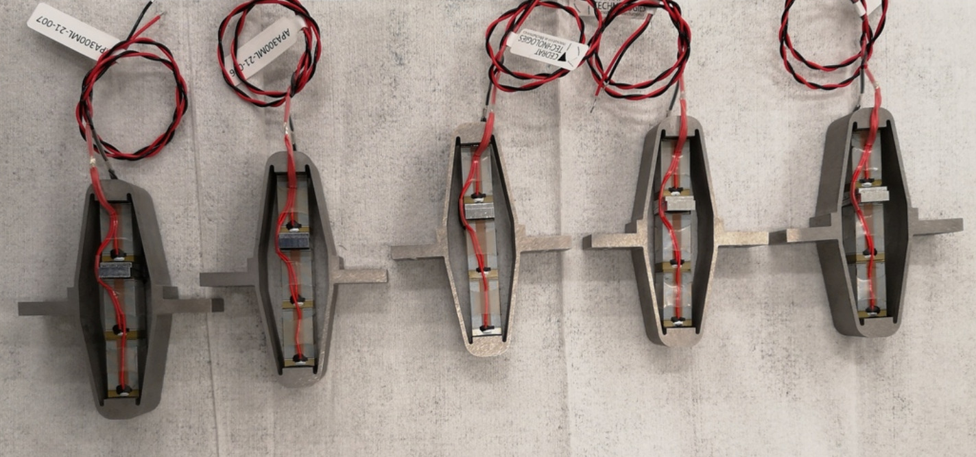
In this chapter, the goal is to ensure that the received APA300ML (shown in Figure ref:fig:test_apa_received) are complying with the requirements and that the dynamical models of the actuator accurately represent its dynamics.
In section ref:sec:test_apa_basic_meas, the mechanical tolerances of the APA300ML interfaces are checked together with the electrical properties of the piezoelectric stacks and the achievable stroke. The flexible modes of the APA300ML, which were estimated using a finite element model, are compared with measurements.
Using a dedicated test bench, dynamical measurements are performed (Section ref:sec:test_apa_dynamics). The dynamics from the generated DAC voltage (going through the voltage amplifier and then to two actuator stacks) to the induced axial displacement and to the measured voltage across the force sensor stack are estimated. Integral Force Feedback is experimentally applied, and the damped plants are estimated for several feedback gains.
Two different models of the APA300ML are presented. First, in Section ref:sec:test_apa_model_2dof, a two degrees-of-freedom model is presented, tuned, and compared with the measured dynamics. This model is proven to accurately represent the APA300ML's axial dynamics while having low complexity.
Then, in Section ref:sec:test_apa_model_flexible, a super element of the APA300ML is extracted using a finite element model and imported into the multi-body model. This more complex model also captures well capture the axial dynamics of the APA300ML.
First Basic Measurements
<<sec:test_apa_basic_meas>>
Introduction ignore
Before measuring the dynamical characteristics of the APA300ML, simple measurements are performed. First, the tolerances (especially flatness) of the mechanical interfaces are checked in Section ref:ssec:test_apa_geometrical_measurements. Then, the capacitance of the piezoelectric stacks is measured in Section ref:ssec:test_apa_electrical_measurements. The achievable stroke of the APA300ML is measured using a displacement probe in Section ref:ssec:test_apa_stroke_measurements. Finally, in Section ref:ssec:test_apa_spurious_resonances, the flexible modes of the APA are measured and compared with a finite element model.
Geometrical Measurements
<<ssec:test_apa_geometrical_measurements>>
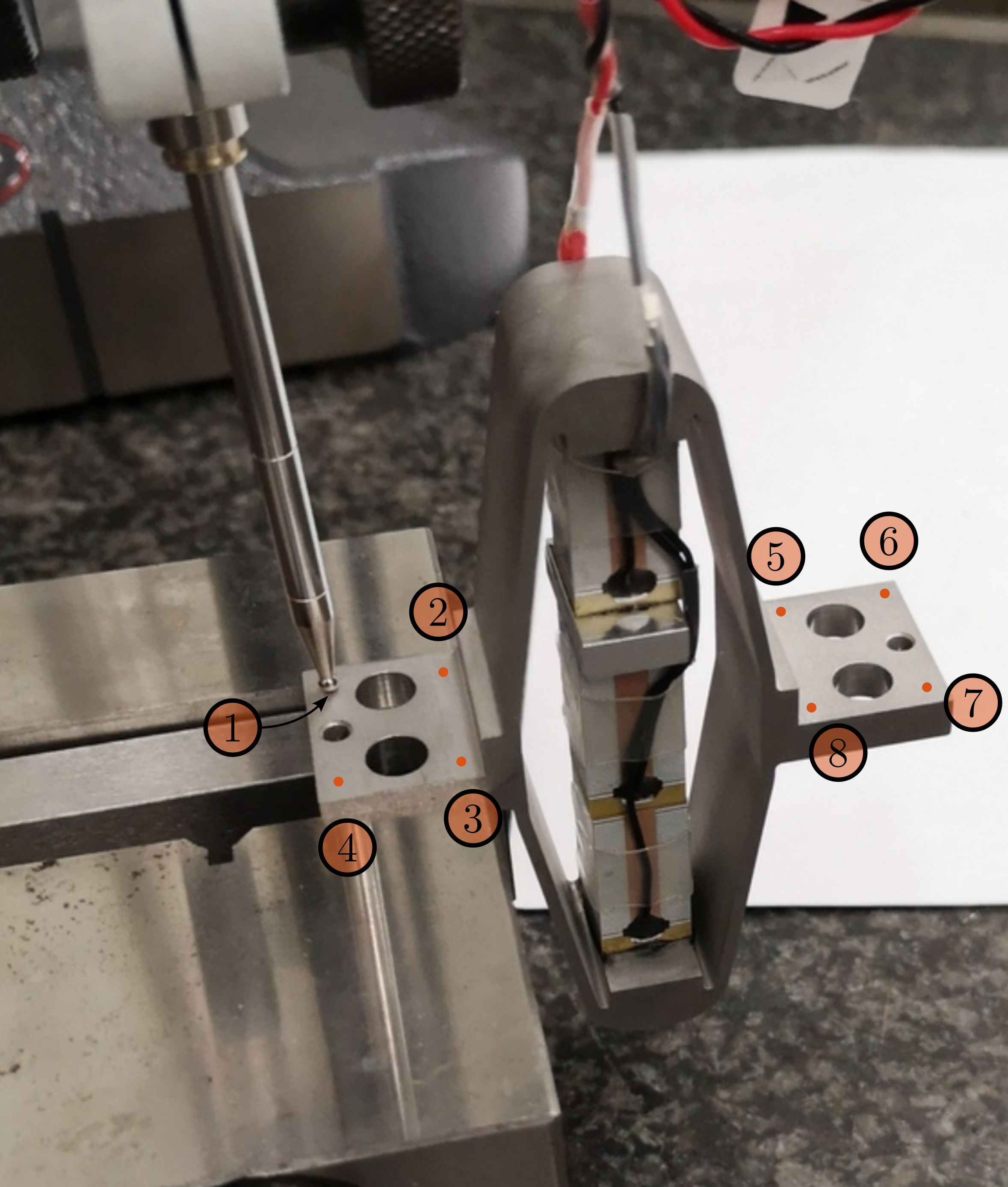
To measure the flatness of the two mechanical interfaces of the APA300ML, a small measurement bench is installed on top of a metrology granite with excellent flatness. As shown in Figure ref:fig:test_apa_flatness_setup, the APA is fixed to a clamp while a measuring probe1 is used to measure the height of four points on each of the APA300ML interfaces. From the X-Y-Z coordinates of the measured eight points, the flatness is estimated by best fitting2 a plane through all the points. The measured flatness values, summarized in Table ref:tab:test_apa_flatness_meas, are within the specifications.
%% Measured height for all the APA at the 8 locations
apa1 = 1e-6*[0, -0.5 , 3.5  , 3.5  , 42   , 45.5, 52.5 , 46];
apa2 = 1e-6*[0, -2.5 , -3   , 0    , -1.5 , 1   , -2   , -4];
apa3 = 1e-6*[0, -1.5 , 15   , 17.5 , 6.5  , 6.5 , 21   , 23];
apa4 = 1e-6*[0, 6.5  , 14.5 , 9    , 16   , 22  , 29.5 , 21];
apa5 = 1e-6*[0, -12.5, 16.5 , 28.5 , -43  , -52 , -22.5, -13.5];
apa6 = 1e-6*[0, -8   , -2   , 5    , -57.5, -62 , -55.5, -52.5];
apa7 = 1e-6*[0, 9    , -18.5, -30  , 31   , 46.5, 16.5 , 7.5];

apa = {apa1, apa2, apa3, apa4, apa5, apa6, apa7};

%% X-Y positions of the measurements points
W = 20e-3;   % Width [m]
L = 61e-3;   % Length [m]
d = 1e-3;    % Distance from border [m]
l = 15.5e-3; % [m]

pos = [[-L/2 + d,      W/2 - d];
       [-L/2 + l - d,  W/2 - d];
       [-L/2 + l - d, -W/2 + d];
       [-L/2 + d,     -W/2 + d];
       [L/2 - l + d,   W/2 - d];
       [L/2 - d,       W/2 - d];
       [L/2 - d,      -W/2 + d];
       [L/2 - l + d,  -W/2 + d]]';

%% Using fminsearch to find the best fitting plane
apa_d = zeros(1, 7); % Measured flatness of the APA
for i = 1:7
    fun = @(x)max(abs(([pos; apa{i}]-[0;0;x(1)])'*([x(2:3);1]/norm([x(2:3);1]))));
    x0 = [0;0;0];
    [x, min_d] = fminsearch(fun,x0);
    apa_d(i) = min_d;
end\hfill
| Flatness $[\mu m]$ | |
|---|---|
| APA 1 | 8.9 |
| APA 2 | 3.1 |
| APA 3 | 9.1 |
| APA 4 | 3.0 |
| APA 5 | 1.9 |
| APA 6 | 7.1 |
| APA 7 | 18.7 |
Electrical Measurements
<<ssec:test_apa_electrical_measurements>>
From the documentation of the APA300ML, the total capacitance of the three stacks should be between $18\,\mu F$ and $26\,\mu F$ with a nominal capacitance of $20\,\mu F$.
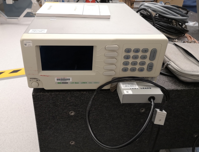
The capacitance of the APA300ML piezoelectric stacks was measured with the LCR meter3 shown in Figure ref:fig:test_apa_lcr_meter. The two stacks used as the actuator and the stack used as the force sensor were measured separately. The measured capacitance values are summarized in Table ref:tab:test_apa_capacitance and the average capacitance of one stack is $\approx 5 \mu F$. However, the measured capacitance of the stacks of "APA 3" is only half of the expected capacitance. This may indicate a manufacturing defect.
The measured capacitance is found to be lower than the specified value. This may be because the manufacturer measures the capacitance with large signals ($-20\,V$ to $150\,V$), whereas it was here measured with small signals cite:&wehrsdorfer95_large_signal_measur_piezoel_stack.
\hfill
| Sensor Stack | Actuator Stacks | |
|---|---|---|
| APA 1 | 5.10 | 10.03 |
| APA 2 | 4.99 | 9.85 |
| APA 3 | 1.72 | 5.18 |
| APA 4 | 4.94 | 9.82 |
| APA 5 | 4.90 | 9.66 |
| APA 6 | 4.99 | 9.91 |
| APA 7 | 4.85 | 9.85 |
Stroke and Hysteresis Measurement
<<ssec:test_apa_stroke_measurements>>
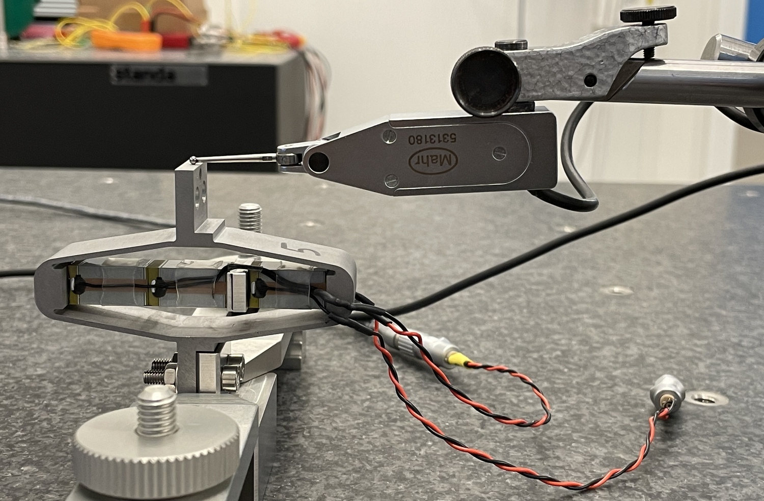
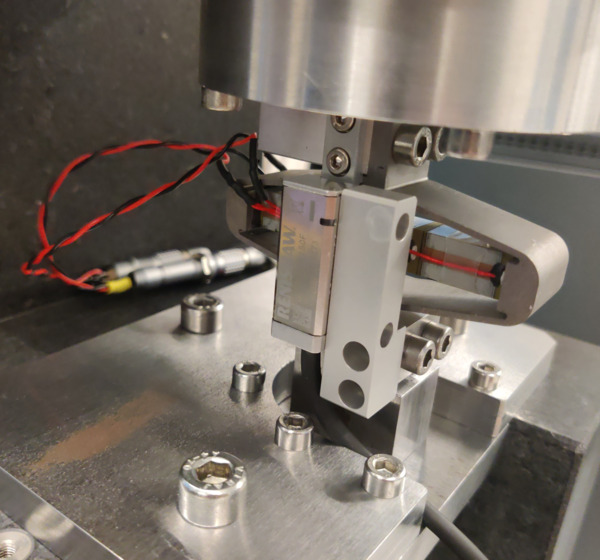
To compare the stroke of the APA300ML with the datasheet specifications, one side of the APA is fixed to the granite, and a displacement probe4 is located on the other side as shown in Figure ref:fig:test_apa_stroke_bench.
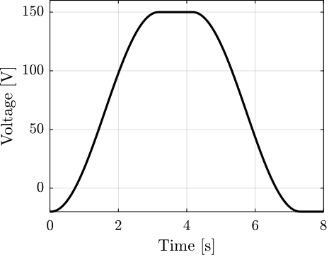
The voltage across the two actuator stacks is varied from $-20\,V$ to $150\,V$ using a DAC5 and a voltage amplifier6. Note that the voltage is slowly varied as the displacement probe has a very low measurement bandwidth (see Figure ref:fig:test_apa_stroke_voltage).
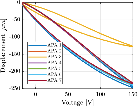
The measured APA displacement is shown as a function of the applied voltage in Figure ref:fig:test_apa_stroke_hysteresis. Typical hysteresis curves for piezoelectric stack actuators can be observed. The measured stroke is approximately $250\,\mu m$ when using only two of the three stacks. This is even above what is specified as the nominal stroke in the data-sheet ($304\,\mu m$, therefore $\approx 200\,\mu m$ if only two stacks are used). For the NASS, this stroke is sufficient because the positioning errors to be corrected using the nano-hexapod are expected to be in the order of $10\,\mu m$.
It is clear from Figure ref:fig:test_apa_stroke_hysteresis that "APA 3" has an issue compared with the other units. This confirms the abnormal electrical measurements made in Section ref:ssec:test_apa_electrical_measurements. This unit was sent sent back to Cedrat, and a new one was shipped back. From now on, only the six remaining amplified piezoelectric actuators that behave as expected will be used.
%% Load the measured strokes
load('meas_apa_stroke.mat', 'apa300ml_2s')
Flexible Mode Measurement
<<ssec:test_apa_spurious_resonances>>
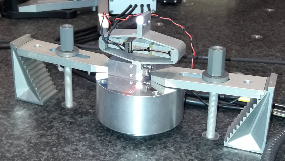
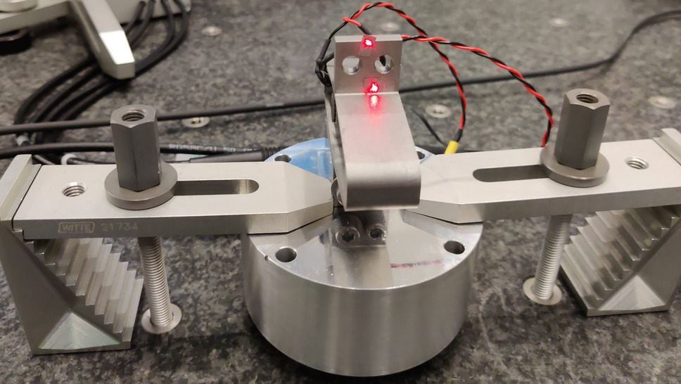
In this section, the flexible modes of the APA300ML are investigated both experimentally and using a Finite Element Model. To experimentally estimate these modes, the APA is fixed at one end (see Figure ref:fig:test_apa_meas_setup_modes). A Laser Doppler Vibrometer7 is used to measure the difference of motion between two "red" points and an instrumented hammer8 is used to excite the flexible modes. Using this setup, the transfer function from the injected force to the measured rotation can be computed under different conditions, and the frequency and mode shapes of the flexible modes can be estimated.
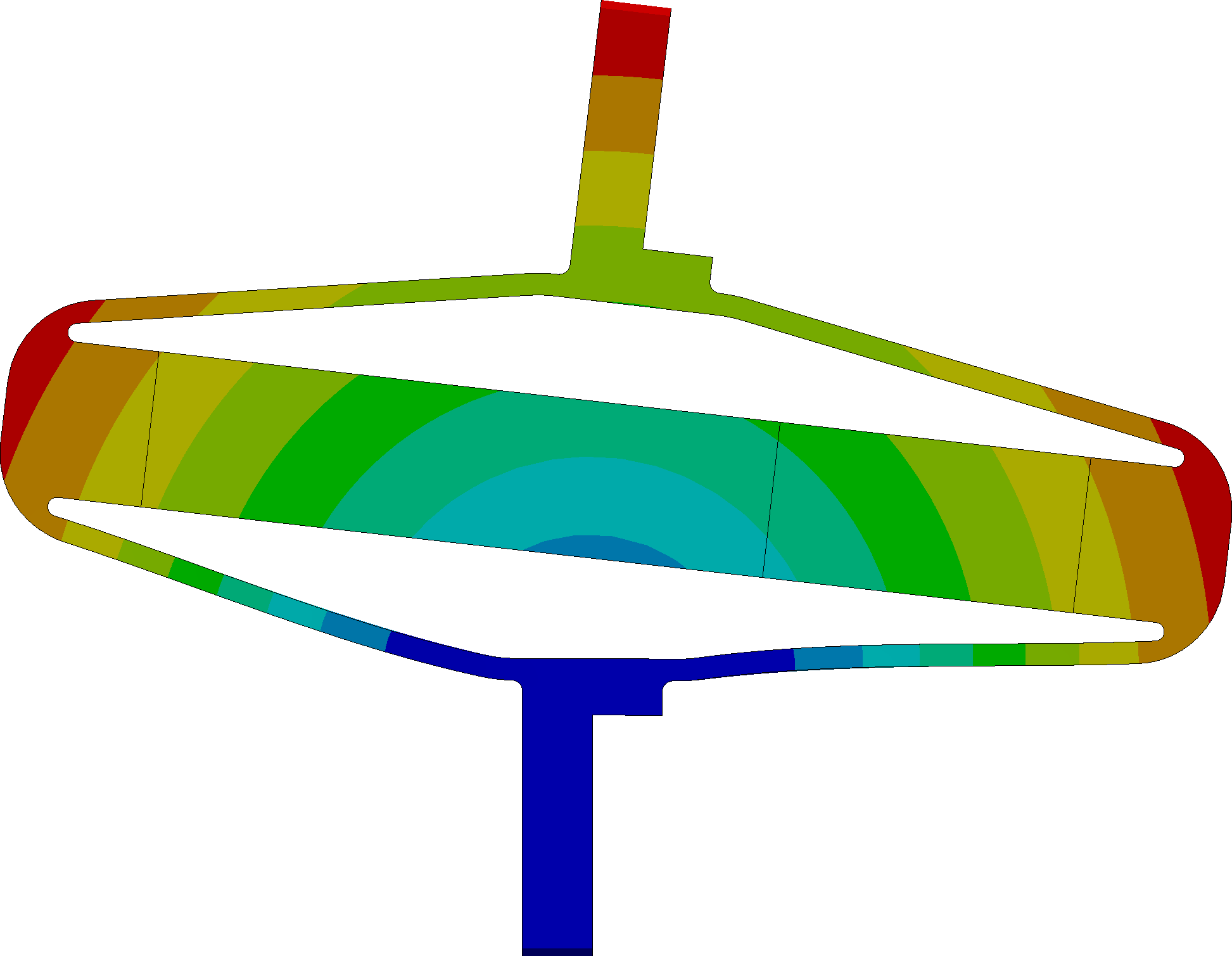
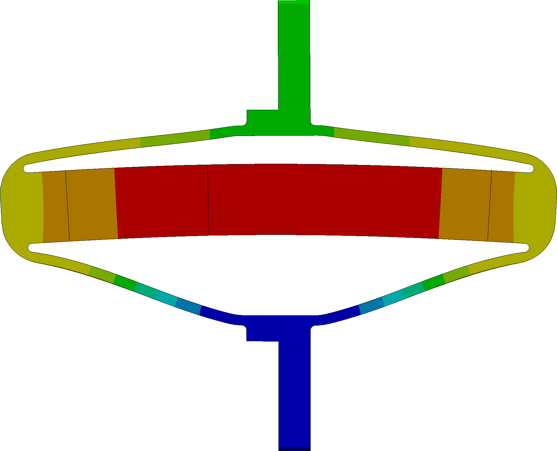
The flexible modes for the same condition (i.e. one mechanical interface of the APA300ML fixed) are estimated using a finite element software, and the results are shown in Figure ref:fig:test_apa_mode_shapes.
%% X-Bending Identification
% Load Data
bending_X = load('apa300ml_bending_X_top.mat');

% Spectral Analysis setup
Ts = bending_X.Track1_X_Resolution; % Sampling Time [s]
Nfft = floor(1/Ts);
win = hanning(Nfft);
Noverlap = floor(Nfft/2);

% Compute the transfer function from applied force to measured rotation
[G_bending_X, f]  = tfestimate(bending_X.Track1, bending_X.Track2, win, Noverlap, Nfft, 1/Ts);

%% Y-Bending identification
% Load Data
bending_Y = load('apa300ml_bending_Y_top.mat');

% Compute the transfer function
[G_bending_Y, ~]  = tfestimate(bending_Y.Track1, bending_Y.Track2, win, Noverlap, Nfft, 1/Ts);
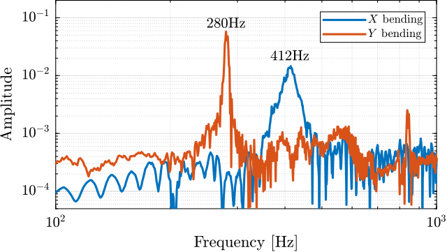
The measured frequency response functions computed from the experimental setups of figures ref:fig:test_apa_meas_setup_X_bending and ref:fig:test_apa_meas_setup_Y_bending are shown in Figure ref:fig:test_apa_meas_freq_compare. The $y$ bending mode is observed at $280\,\text{Hz}$ and the $x$ bending mode is at $412\,\text{Hz}$. These modes are measured at higher frequencies than the frequencies estimated from the Finite Element Model (see frequencies in Figure ref:fig:test_apa_mode_shapes). This is the opposite of what is usually observed (i.e. having lower resonance frequencies in practice than the estimation from a finite element model). This could be explained by underestimation of the Young's modulus of the steel used for the shell (190 GPa was used for the model, but steel with Young's modulus of 210 GPa could have been used). Another explanation is the shape difference between the manufactured APA300ML and the 3D model, for instance thicker blades.
Dynamical measurements
<<sec:test_apa_dynamics>>
Introduction ignore
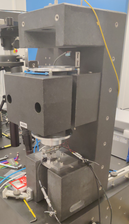
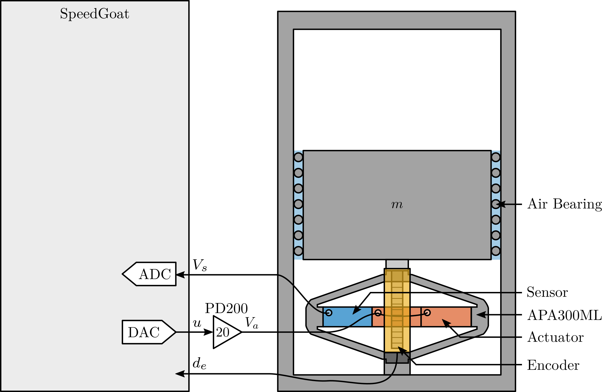
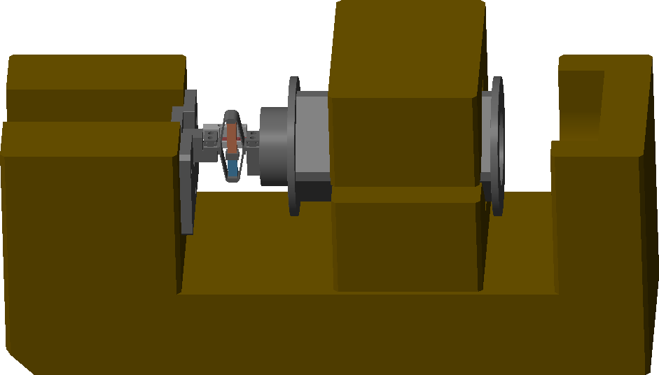
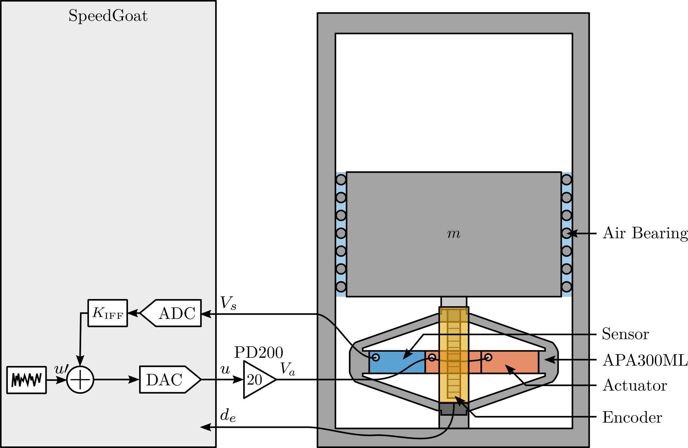
After the measurements on the APA were performed in Section ref:sec:test_apa_basic_meas, a new test bench was used to better characterize the dynamics of the APA300ML. This test bench, depicted in Figure ref:fig:test_bench_apa, comprises the APA300ML fixed at one end to a stationary granite block and at the other end to a 5kg granite block that is vertically guided by an air bearing. Thus, there is no friction when actuating the APA300ML, and it will be easier to characterize its behavior independently of other factors. An encoder9 is used to measure the relative movement between the two granite blocks, thereby measuring the axial displacement of the APA.
The bench is schematically shown in Figure ref:fig:test_apa_schematic with the associated signals. It will be first used to estimate the hysteresis from the piezoelectric stack (Section ref:ssec:test_apa_hysteresis) as well as the axial stiffness of the APA300ML (Section ref:ssec:test_apa_stiffness). The frequency response functions from the DAC voltage $u$ to the displacement $d_e$ and to the voltage $V_s$ are measured in Section ref:ssec:test_apa_meas_dynamics. The presence of a non-minimum phase zero found on the transfer function from $u$ to $V_s$ is investigated in Section ref:ssec:test_apa_non_minimum_phase. To limit the low-frequency gain of the transfer function from $u$ to $V_s$, a resistor is added across the force sensor stack (Section ref:ssec:test_apa_resistance_sensor_stack). Finally, the Integral Force Feedback is implemented, and the amount of damping added is experimentally estimated in Section ref:ssec:test_apa_iff_locus.
Hysteresis
<<ssec:test_apa_hysteresis>>
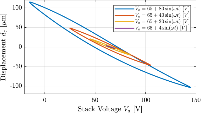
Because the payload is vertically guided without friction, the hysteresis of the APA can be estimated from the motion of the payload. A quasi static10 sinusoidal excitation $V_a$ with an offset of $65\,V$ (halfway between $-20\,V$ and $150\,V$) and with an amplitude varying from $4\,V$ up to $80\,V$ is generated using the DAC. For each excitation amplitude, the vertical displacement $d_e$ of the mass is measured and displayed as a function of the applied voltage in Figure ref:fig:test_apa_meas_hysteresis. This is the typical behavior expected from a PZT stack actuator, where the hysteresis increases as a function of the applied voltage amplitude cite:&fleming14_desig_model_contr_nanop_system chap. 1.4.
%% Load measured data - hysteresis
apa_hyst = load('frf_data_1_hysteresis.mat', 't', 'u', 'de');

% Initial time set to zero
apa_hyst.t = apa_hyst.t - apa_hyst.t(1);

ampls = [0.1, 0.2, 0.4, 1, 2, 4]; % Excitation voltage amplitudesAxial stiffness
<<ssec:test_apa_stiffness>>
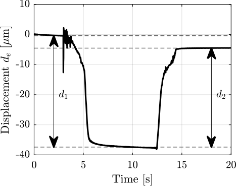
To estimate the stiffness of the APA, a weight with known mass $m_a = 6.4\,\text{kg}$ is added on top of the suspended granite and the deflection $\Delta d_e$ is measured using the encoder. The APA stiffness can then be estimated from equation eqref:eq:test_apa_stiffness, with $g \approx 9.8\,m/s^2$ the acceleration of gravity.
\begin{equation} \label{eq:test_apa_stiffness} k_{\text{apa}} = \frac{m_a g}{Δ d_e}
\end{equation}
%% Load data for stiffness measurement
apa_nums = [1 2 4 5 6 8];
apa_mass = {};
for i = 1:length(apa_nums)
    apa_mass(i) = {load(sprintf('frf_data_%i_add_mass_closed_circuit.mat', apa_nums(i)), 't', 'de')};
    % The initial displacement is set to zero
    apa_mass{i}.de = apa_mass{i}.de - mean(apa_mass{i}.de(apa_mass{i}.t<11));
end

added_mass = 6.4; % Added mass [kg]
The measured displacement $d_e$ as a function of time is shown in Figure ref:fig:test_apa_meas_stiffness_time. It can be seen that there are some drifts in the measured displacement (probably due to piezoelectric creep), and that the displacement does not return to the initial position after the mass is removed (probably due to piezoelectric hysteresis). These two effects induce some uncertainties in the measured stiffness.
The stiffnesses are computed for all APAs from the two displacements $d_1$ and $d_2$ (see Figure ref:fig:test_apa_meas_stiffness_time) leading to two stiffness estimations $k_1$ and $k_2$. These estimated stiffnesses are summarized in Table ref:tab:test_apa_measured_stiffnesses and are found to be close to the specified nominal stiffness of the APA300ML $k = 1.8\,N/\mu m$.
\hfill
| APA | $k_1$ | $k_2$ |
|---|---|---|
| 1 | 1.68 | 1.9 |
| 2 | 1.69 | 1.9 |
| 4 | 1.7 | 1.91 |
| 5 | 1.7 | 1.93 |
| 6 | 1.7 | 1.92 |
| 8 | 1.73 | 1.98 |
The stiffness can also be computed using equation eqref:eq:test_apa_res_freq by knowing the main vertical resonance frequency $\omega_z \approx 95\,\text{Hz}$ (estimated by the dynamical measurements shown in section ref:ssec:test_apa_meas_dynamics) and the suspended mass $m_{\text{sus}} = 5.7\,\text{kg}$.
\begin{equation} \label{eq:test_apa_res_freq} ω_z = \sqrt{\frac{k}{m_{\text{sus}}}}
\end{equation}
The obtained stiffness is $k \approx 2\,N/\mu m$ which is close to the values found in the documentation and using the "static deflection" method.
It is important to note that changes to the electrical impedance connected to the piezoelectric stacks affect the mechanical compliance (or stiffness) of the piezoelectric stack cite:&reza06_piezoel_trans_vibrat_contr_dampin chap. 2.
To estimate this effect for the APA300ML, its stiffness is estimated using the "static deflection" method in two cases:
- $k_{\text{os}}$: piezoelectric stacks left unconnected (or connect to the high impedance ADC)
- $k_{\text{sc}}$: piezoelectric stacks short-circuited (or connected to the voltage amplifier with small output impedance)
The open-circuit stiffness is estimated at $k_{\text{oc}} \approx 2.3\,N/\mu m$ while the closed-circuit stiffness $k_{\text{sc}} \approx 1.7\,N/\mu m$.
%% Load Data
add_mass_oc = load('frf_data_1_add_mass_open_circuit.mat',   't', 'de');
add_mass_cc = load('frf_data_1_add_mass_closed_circuit.mat', 't', 'de');

%% Zero displacement at initial time
add_mass_oc.de = add_mass_oc.de - mean(add_mass_oc.de(add_mass_oc.t<11));
add_mass_cc.de = add_mass_cc.de - mean(add_mass_cc.de(add_mass_cc.t<11));

%% Estimation of the stiffness in Open Circuit and Closed-Circuit
apa_k_oc = 9.8 * added_mass / (mean(add_mass_oc.de(add_mass_oc.t > 12 & add_mass_oc.t < 12.5)) - mean(add_mass_oc.de(add_mass_oc.t > 20 & add_mass_oc.t < 20.5)));
apa_k_sc = 9.8 * added_mass / (mean(add_mass_cc.de(add_mass_cc.t > 12 & add_mass_cc.t < 12.5)) - mean(add_mass_cc.de(add_mass_cc.t > 20 & add_mass_cc.t < 20.5)));
Dynamics
<<ssec:test_apa_meas_dynamics>>
%% Identification using sweep sine (low frequency)
load('frf_data_sweep.mat');
load('frf_data_noise_hf.mat');

%% Sampling Frequency
Ts = 1e-4; % Sampling Time [s]
Fs = 1/Ts; % Sampling Frequency [Hz]

%% "Hanning" windows used for the spectral analysis:
Nfft = floor(2/Ts);
win = hanning(Nfft);
Noverlap = floor(Nfft/2);

%% Separation of frequencies: low freqs using sweep sine, and high freq using noise
% Only used to have the frequency vector "f"
[~, f] = tfestimate(apa_sweep{1}.u, apa_sweep{1}.de, win, Noverlap, Nfft, 1/Ts);
i_lf = f <= 350;
i_hf = f >  350;

%% FRF estimation of the transfer function from u to de
enc_frf = zeros(length(f), length(apa_nums));
for i = 1:length(apa_nums)
    [frf_lf, ~] = tfestimate(apa_sweep{i}.u,    apa_sweep{i}.de,    win, Noverlap, Nfft, 1/Ts);
    [frf_hf, ~] = tfestimate(apa_noise_hf{i}.u, apa_noise_hf{i}.de, win, Noverlap, Nfft, 1/Ts);
    enc_frf(:, i) = [frf_lf(i_lf); frf_hf(i_hf)];
end

%% FRF estimation of the transfer function from u to Vs
iff_frf = zeros(length(f), length(apa_nums));
for i = 1:length(apa_nums)
    [frf_lf, ~] = tfestimate(apa_sweep{i}.u,    apa_sweep{i}.Vs,    win, Noverlap, Nfft, 1/Ts);
    [frf_hf, ~] = tfestimate(apa_noise_hf{i}.u, apa_noise_hf{i}.Vs, win, Noverlap, Nfft, 1/Ts);
    iff_frf(:, i) = [frf_lf(i_lf); frf_hf(i_hf)];
end
%% Save the identified dynamics for further analysis
save('mat/meas_apa_frf.mat', 'f', 'Ts', 'enc_frf', 'iff_frf', 'apa_nums');In this section, the dynamics from the excitation voltage $u$ to the encoder measured displacement $d_e$ and to the force sensor voltage $V_s$ is identified.
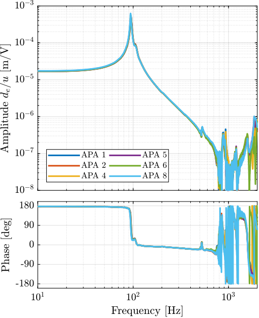
First, the dynamics from $u$ to $d_e$ for the six APA300ML are compared in Figure ref:fig:test_apa_frf_encoder. The obtained frequency response functions are similar to those of a (second order) mass-spring-damper system with:
- A "stiffness line" indicating a static gain equal to $\approx -17\,\mu m/V$. The negative sign comes from the fact that an increase in voltage stretches the piezoelectric stack which reduces the height of the APA
- A lightly damped resonance at $95\,\text{Hz}$
- A "mass line" up to $\approx 800\,\text{Hz}$, above which additional resonances appear. These additional resonances might be due to the limited stiffness of the encoder support or from the limited compliance of the APA support. The flexible modes studied in section ref:ssec:test_apa_spurious_resonances seem not to impact the measured axial motion of the actuator.
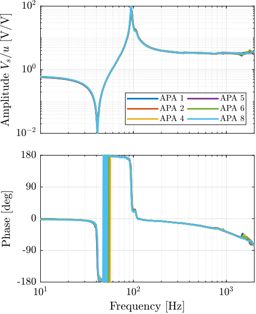
The dynamics from $u$ to the measured voltage across the sensor stack $V_s$ for the six APA300ML are compared in Figure ref:fig:test_apa_frf_force.
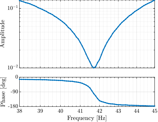
A lightly damped resonance (pole) is observed at $95\,\text{Hz}$ and a lightly damped anti-resonance (zero) at $41\,\text{Hz}$. No additional resonances are present up to at least $2\,\text{kHz}$ indicating that Integral Force Feedback can be applied without stability issues from high-frequency flexible modes. The zero at $41\,\text{Hz}$ seems to be non-minimum phase (the phase decreases by 180 degrees whereas it should have increased by 180 degrees for a minimum phase zero). This is investigated in Section ref:ssec:test_apa_non_minimum_phase.
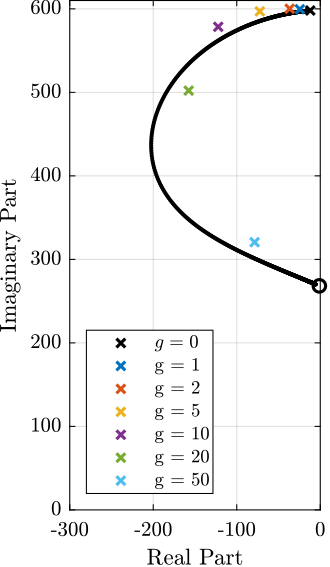
As illustrated by the Root Locus plot, the poles of the closed-loop system converges to the zeros of the open-loop plant as the feedback gain increases. The significance of this behavior varies with the type of sensor used, as explained in cite:&preumont18_vibrat_contr_activ_struc_fourt_edition chap. 7.6. Considering the transfer function from $u$ to $V_s$, if a controller with a very high gain is applied such that the sensor stack voltage $V_s$ is kept at zero, the sensor (and by extension, the actuator stacks since they are in series) experiences negligible stress and strain. Consequently, the closed-loop system virtually corresponds to one in which the piezoelectric stacks are absent, leaving only the mechanical shell. From this analysis, it can be inferred that the axial stiffness of the shell is $k_{\text{shell}} = m \omega_0^2 = 5.7 \cdot (2\pi \cdot 41)^2 = 0.38\,N/\mu m$ (which is close to what is found using a finite element model).
All the identified dynamics of the six APA300ML (both when looking at the encoder in Figure ref:fig:test_apa_frf_encoder and at the force sensor in Figure ref:fig:test_apa_frf_force) are almost identical, indicating good manufacturing repeatability for the piezoelectric stacks and the mechanical shell.
Non Minimum Phase Zero?
<<ssec:test_apa_non_minimum_phase>>
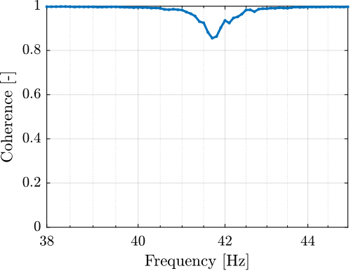
It was surprising to observe a non-minimum phase zero on the transfer function from $u$ to $V_s$ (Figure ref:fig:test_apa_frf_force). It was initially thought that this non-minimum phase behavior was an artifact arising from the measurement. A longer measurement was performed using different excitation signals (noise, slow sine sweep, etc.) to determine if the phase behavior of the zero changes (Figure ref:fig:test_apa_non_minimum_phase). The coherence (Figure ref:fig:test_apa_non_minimum_phase_coherence) is good even in the vicinity of the lightly damped zero, and the phase (Figure ref:fig:test_apa_non_minimum_phase_zoom) clearly indicates non-minimum phase behavior.
Such non-minimum phase zero when using load cells has also been observed on other mechanical systems cite:&spanos95_soft_activ_vibrat_isolat;&thayer02_six_axis_vibrat_isolat_system;&hauge04_sensor_contr_space_based_six. It could be induced to small non-linearity in the system, but the reason for this non-minimum phase for the APA300ML is not yet clear.
However, this is not so important here because the zero is lightly damped (i.e. very close to the imaginary axis), and the closed loop poles (see the Root Locus plot in Figure ref:fig:test_apa_iff_root_locus) should not be unstable, except for very large controller gains that will never be applied in practice.
%% Long measurement
long_noise = load('frf_struts_align_3_noise_long.mat', 't', 'u', 'Vs');

% Long window for fine frequency axis
Ts = 1e-4; % Sampling Time [s]
Nfft = floor(10/Ts);
win = hanning(Nfft);
Noverlap = floor(Nfft/2);

% Transfer function estimation
[frf_noise, f] = tfestimate(long_noise.u, long_noise.Vs, win, Noverlap, Nfft, 1/Ts);
[coh_noise, ~] = mscohere(long_noise.u, long_noise.Vs, win, Noverlap, Nfft, 1/Ts);
Effect of the resistor on the IFF Plant
<<ssec:test_apa_resistance_sensor_stack>>
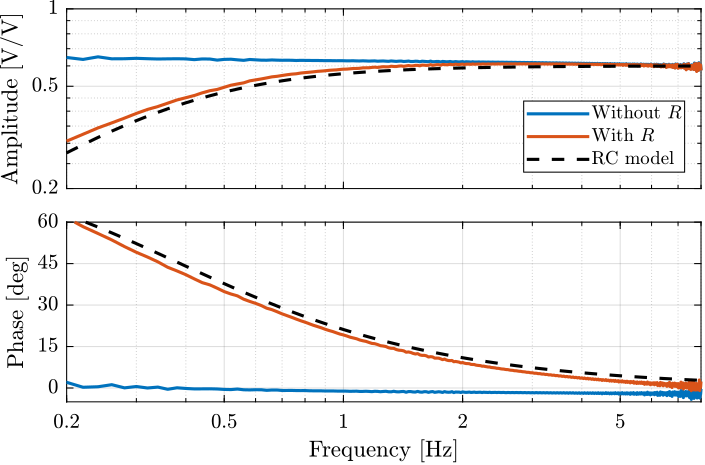
A resistor $R \approx 80.6\,k\Omega$ is added in parallel with the sensor stack, which forms a high-pass filter with the capacitance of the piezoelectric stack (capacitance estimated at $\approx 5\,\mu F$).
As explained before, this is done to limit the voltage offset due to the input bias current of the ADC as well as to limit the low frequency gain.
The (low frequency) transfer function from $u$ to $V_s$ with and without this resistor were measured and compared in Figure ref:fig:test_apa_effect_resistance. It is confirmed that the added resistor has the effect of adding a high-pass filter with a cut-off frequency of $\approx 0.39\,\text{Hz}$.
%% Load the data
wi_k = load('frf_data_1_sweep_lf_with_R.mat', 't', 'Vs', 'u'); % With the resistor
wo_k = load('frf_data_1_sweep_lf.mat',        't', 'Vs', 'u'); % Without the resistor

%% Large Hanning window for good low frequency estimate
Nfft = floor(50/Ts);
win = hanning(Nfft);
Noverlap = floor(Nfft/2);

%% Compute the transfer functions from u to Vs
[frf_wo_k, f] = tfestimate(wo_k.u, wo_k.Vs, win, Noverlap, Nfft, 1/Ts);
[frf_wi_k, ~] = tfestimate(wi_k.u, wi_k.Vs, win, Noverlap, Nfft, 1/Ts);

%% Model for the high pass filter
C = 5.1e-6; % Sensor Stack capacitance [F]
R = 80.6e3; % Parallel Resistor [Ohm]

f0 = 1/(2*pi*R*C); % Crossover frequency of RC HPF [Hz]

G_hpf = 0.6*(s/(2*pi*f0))/(1 + s/(2*pi*f0));Integral Force Feedback
<<ssec:test_apa_iff_locus>>
%% Load identification Data
data = load("2023-03-17_11-28_iff_plant.mat");

%% Spectral Analysis setup
Ts = 1e-4; % Sampling Time [s]
Nfft = floor(5/Ts);
win = hanning(Nfft);
Noverlap = floor(Nfft/2);

%% Compute the transfer function from applied force to measured rotation
[G_iff, f]  = tfestimate(data.id_plant, data.Vs, win, Noverlap, Nfft, 1/Ts);
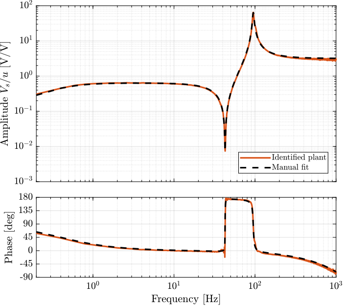
To implement the Integral Force Feedback strategy, the measured frequency response function from $u$ to $V_s$ (Figure ref:fig:test_apa_frf_force) is fitted using the transfer function shown in equation eqref:eq:test_apa_iff_manual_fit. The parameters were manually tuned, and the obtained values are $\omega_{\textsc{hpf}} = 0.4\, \text{Hz}$, $\omega_{z} = 42.7\, \text{Hz}$, $\xi_{z} = 0.4\,\%$, $\omega_{p} = 95.2\, \text{Hz}$, $\xi_{p} = 2\,\%$ and $g_0 = 0.64$.
\begin{equation} \label{eq:test_apa_iff_manual_fit} G_{\textsc{iff},m}(s) = g_0 ⋅ \frac{1 + 2 ξ_z \frac{s}{ω_z} + \frac{s^2}{ω_z^2}}{1 + 2 ξ_p \frac{s}{ω_p} + \frac{s^2}{ω_p^2}} ⋅ \frac{s}{ω_{\textsc{hpf}} + s}
\end{equation}
A comparison between the identified plant and the manually tuned transfer function is shown in Figure ref:fig:test_apa_iff_plant_comp_manual_fit.
%% Basic manually tuned model
w0z = 2*pi*42.7; % Zero frequency
xiz = 0.004; % Zero damping

w0p = 2*pi*95.2; % Pole frequency
xip = 0.02; % Pole damping

G_iff_model = exp(-2*s*Ts)*0.64*(1 + 2*xiz/w0z*s + s^2/w0z^2)/(1 + 2*xip/w0p*s + s^2/w0p^2)*(s/(s+2*pi*0.4));The implemented Integral Force Feedback Controller transfer function is shown in equation eqref:eq:test_apa_Kiff_formula. It contains a high-pass filter (cut-off frequency of $2\,\text{Hz}$) to limit the low-frequency gain, a low-pass filter to add integral action above $20\,\text{Hz}$, a second low-pass filter to add robustness to high-frequency resonances, and a tunable gain $g$.
\begin{equation} \label{eq:test_apa_Kiff_formula} K_{\textsc{iff}}(s) = -10 ⋅ g ⋅ \frac{s}{s + 2π ⋅ 2} ⋅ \frac{1}{s + 2π ⋅ 20} ⋅ \frac{1}{s + 2π⋅ 2000}
\end{equation}
%% Integral Force Feedback Controller
K_iff = -10*(1/(s + 2*pi*20)) * ... % LPF: provides integral action above 20Hz
            (s/(s + 2*pi*2))  * ... % HPF: limit low frequency gain
            (1/(1 + s/2/pi/2e3));   % LPF: more robust to high frequency resonances
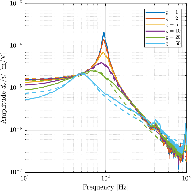
To estimate how the dynamics of the APA changes when the Integral Force Feedback controller is implemented, the test bench shown in Figure ref:fig:test_apa_iff_schematic is used. The transfer function from the "damped" plant input $u\prime$ to the encoder displacement $d_e$ is identified for several IFF controller gains $g$.
%% Load Data
data = load("2023-03-17_14-10_damped_plants_new.mat");

%% Spectral Analysis setup
Ts = 1e-4; % Sampling Time [s]
Nfft = floor(1/Ts);
win = hanning(Nfft);
Noverlap = floor(Nfft/2);

%% Get the frequency vector
[~, f]  = tfestimate(data.data(1).id_plant(1:end), data.data(1).dL(1:end), win, Noverlap, Nfft, 1/Ts);

%% Gains used for analysis are between 1 and 50
i_kept = [5:10];

%% Identify the damped plant from u' to de for different IFF gains
G_dL_frf = {zeros(1,length(i_kept))};

for i = 1:length(i_kept)
    [G_dL, ~]  = tfestimate(data.data(i_kept(i)).id_plant(1:end), data.data(i_kept(i)).dL(1:end), win, Noverlap, Nfft, 1/Ts);
    G_dL_frf(i) = {G_dL};
end
The identified dynamics were then fitted by second order transfer functions11. A comparison between the identified damped dynamics and the fitted second-order transfer functions is shown in Figure ref:fig:test_apa_identified_damped_plants for different gains $g$. It is clear that a large amount of damping is added when the gain is increased and that the frequency of the pole is shifted to lower frequencies.
The evolution of the pole in the complex plane as a function of the controller gain $g$ (i.e. the "root locus") is computed in two cases. First using the IFF plant model eqref:eq:test_apa_iff_manual_fit and the implemented controller eqref:eq:test_apa_Kiff_formula. Second using the fitted transfer functions of the damped plants experimentally identified for several controller gains. The two obtained root loci are compared in Figure ref:fig:test_apa_iff_root_locus and are in good agreement considering that the damped plants were fitted using only a second-order transfer function.
%% Fit the data with 2nd order transfer function using vectfit3
opts = struct();

opts.stable = 1;    % Enforce stable poles
opts.asymp = 1;     % Force D matrix to be null
opts.relax = 1;     % Use vector fitting with relaxed non-triviality constraint
opts.skip_pole = 0; % Do NOT skip pole identification
opts.skip_res = 0;  % Do NOT skip identification of residues (C,D,E)
opts.cmplx_ss = 0;  % Create real state space model with block diagonal A

opts.spy1 = 0;      % No plotting for first stage of vector fitting
opts.spy2 = 0;      % Create magnitude plot for fitting of f(s)

Niter = 100; % Number of iteration.
N = 2; % Order of approximation
poles = [-25 - 1i*60, -25 + 1i*60]; % First get for the pole location

G_dL_id  = {zeros(1,length(i_kept))};

% Identification just between two frequencies
f_keep = (f>5 & f<200);

for i = 1:length(i_kept)
    %% Estimate resonance frequency and damping
    for iter = 1:Niter
        [G_est, poles, ~, frf_est] = vectfit3(G_dL_frf{i}(f_keep).', 1i*2*pi*f(f_keep)', poles, ones(size(f(f_keep)))', opts);
    end
    G_dL_id(i) = {ss(G_est.A, G_est.B, G_est.C, G_est.D)};
end
APA300ML - 2 degrees-of-freedom Model
<<sec:test_apa_model_2dof>>
Introduction ignore
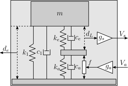
In this section, a multi-body model (Figure ref:fig:test_apa_bench_model) of the measurement bench is used to tune the two degrees-of-freedom model of the APA using the measured frequency response functions.
This two degrees-of-freedom model is developed to accurately represent the APA300ML dynamics while having low complexity and a low number of associated states. After the model is presented, the procedure for tuning the model is described, and the obtained model dynamics is compared with the measurements.
Two degrees-of-freedom APA Model
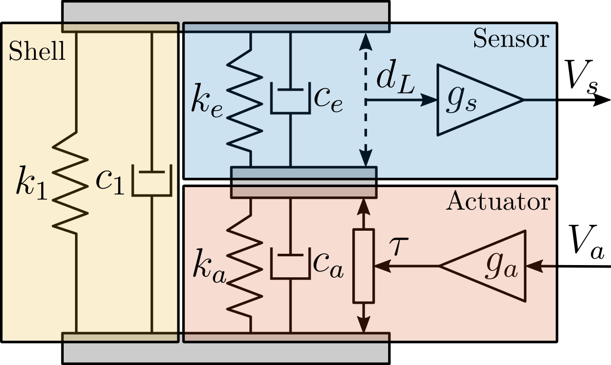
The model of the amplified piezoelectric actuator is shown in Figure ref:fig:test_apa_2dof_model. It can be decomposed into three components:
- the shell whose axial properties are represented by $k_1$ and $c_1$
- the actuator stacks whose contribution to the axial stiffness is represented by $k_a$ and $c_a$. The force source $f$ represents the axial force induced by the force sensor stacks. The sensitivity $g_a$ (in $N/m$) is used to convert the applied voltage $V_a$ to the axial force $f$
- the sensor stack whose contribution to the axial stiffness is represented by $k_e$ and $c_e$. A sensor measures the stack strain $d_e$ which is then converted to a voltage $V_s$ using a sensitivity $g_s$ (in $V/m$)
Such a simple model has some limitations:
- it only represents the axial characteristics of the APA as it is modeled as infinitely rigid in the other directions
- some physical insights are lost, such as the amplification factor and the real stress and strain in the piezoelectric stacks
- the creep and hysteresis of the piezoelectric stacks are not modeled as the model is linear
Tuning of the APA model ignore
9 parameters ($m$, $k_1$, $c_1$, $k_e$, $c_e$, $k_a$, $c_a$, $g_s$ and $g_a$) have to be tuned such that the dynamics of the model (Figure ref:fig:test_apa_2dof_model_simscape) well represents the identified dynamics in Section ref:sec:test_apa_dynamics.
%% Stiffness values for the 2DoF APA model
k1 = 0.38e6; % Estimated Shell Stiffness [N/m]

w0 = 2*pi*95; % Resonance frequency [rad/s]
m = 5.7; % Suspended mass [kg]
ktot = m*(w0)^2; % Total Axial Stiffness to have to wanted resonance frequency [N/m]

ka = 1.5*(ktot-k1); % Stiffness of the (two) actuator stacks [N/m]
ke = 2*ka; % Stiffness of the Sensor stack [N/m]

%% Damping values for the 2DoF APA model
c1 = 5;   % Damping for the Shell [N/(m/s)]
ca = 50;  % Damping of the actuators stacks [N/(m/s)]
ce = 2*ca; % Damping of the sensor stack [N/(m/s)]
%% Estimation ot the sensor and actuator sensitivities
% Initialize the structure with unitary sensor and actuator "sensitivities"
n_hexapod = struct();
n_hexapod.actuator = initializeAPA(...
'type', '2dof', ...
'k', k1, ...
'ka', ka, ...
'ke', ke, ...
'c', c1, ...
'ca', ca, ...
'ce', ce, ...
'Ga', 1, ... % Actuator constant [N/V]
'Gs', 1 ... % Sensor constant [V/m]
);
c_granite = 50; % Do not take into account damping added by the air bearing
% Run the linearization
G_norm = linearize(mdl, io, 0.0, opts);
G_norm.InputName = {'u'};
G_norm.OutputName = {'Vs', 'de'};
% Load Identification Data to estimate the two sensitivities
load('meas_apa_frf.mat', 'f', 'Ts', 'enc_frf', 'iff_frf', 'apa_nums');
% Estimation ot the Actuator sensitivity
fa = 10; % Frequency where the two FRF should match [Hz]
[~, i_f] = min(abs(f - fa));
ga = -abs(enc_frf(i_f,1))./abs(evalfr(G_norm('de', 'u'), 1i*2*pi*fa));
% Estimation ot the Sensor sensitivity
fs = 600; % Frequency where the two FRF should match [Hz]
[~, i_f] = min(abs(f - fs));
gs = -abs(iff_frf(i_f,1))./abs(evalfr(G_norm('Vs', 'u'), 1i*2*pi*fs))/ga;First, the mass $m$ supported by the APA300ML can be estimated from the geometry and density of the different parts or by directly measuring it using a precise weighing scale. Both methods lead to an estimated mass of $m = 5.7\,\text{kg}$.
Then, the axial stiffness of the shell was estimated at $k_1 = 0.38\,N/\mu m$ in Section ref:ssec:test_apa_meas_dynamics from the frequency of the anti-resonance seen on Figure ref:fig:test_apa_frf_force. Similarly, $c_1$ can be estimated from the damping ratio of the same anti-resonance and is found to be close to $5\,Ns/m$.
Then, it is reasonable to assume that the sensor stacks and the two actuator stacks have identical mechanical characteristics12. Therefore, we have $k_e = 2 k_a$ and $c_e = 2 c_a$ as the actuator stack is composed of two stacks in series. In this case, the total stiffness of the APA model is described by eqref:eq:test_apa_2dof_stiffness.
\begin{equation}\label{eq:test_apa_2dof_stiffness} k_{\text{tot}} = k_1 + \frac{k_e k_a}{k_e + k_a} = k_1 + \frac{2}{3} k_a
\end{equation}
Knowing from eqref:eq:test_apa_tot_stiffness that the total stiffness is $k_{\text{tot}} = 2\,N/\mu m$, we get from eqref:eq:test_apa_2dof_stiffness that $k_a = 2.5\,N/\mu m$ and $k_e = 5\,N/\mu m$.
\begin{equation}\label{eq:test_apa_tot_stiffness} ω_0 = \frac{k_{\text{tot}}}{m} \Longrightarrow k_{\text{tot}} = m ω_0^2 = 2\,N/μ m \quad \text{with}\ m = 5.7\,\text{kg}\ \text{and}\ ω_0 = 2π ⋅ 95\, \text{rad}/s
\end{equation}
Then, $c_a$ (and therefore $c_e = 2 c_a$) can be tuned to match the damping ratio of the identified resonance. $c_a = 50\,Ns/m$ and $c_e = 100\,Ns/m$ are obtained.
In the last step, $g_s$ and $g_a$ can be tuned to match the gain of the identified transfer functions.
The obtained parameters of the model shown in Figure ref:fig:test_apa_2dof_model_simscape are summarized in Table ref:tab:test_apa_2dof_parameters.
| Parameter | Value |
|---|---|
| $m$ | $5.7\,\text{kg}$ |
| $k_1$ | $0.38\,N/\mu m$ |
| $k_e$ | $5.0\, N/\mu m$ |
| $k_a$ | $2.5\,N/\mu m$ |
| $c_1$ | $5\,Ns/m$ |
| $c_e$ | $100\,Ns/m$ |
| $c_a$ | $50\,Ns/m$ |
| $g_a$ | $-2.58\,N/V$ |
| $g_s$ | $0.46\,V/\mu m$ |
Obtained Dynamics ignore
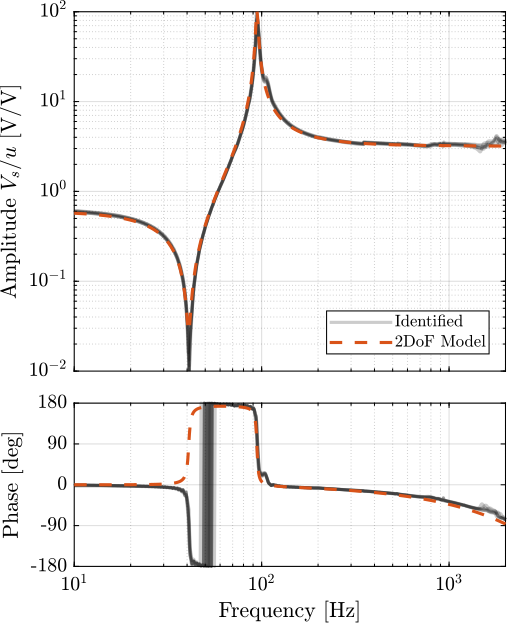
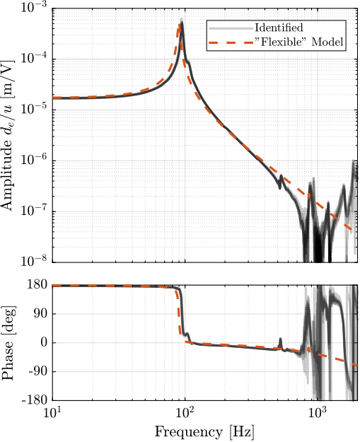
The dynamics of the two degrees-of-freedom model of the APA300ML are extracted using optimized parameters (listed in Table ref:tab:test_apa_2dof_parameters) from the multi-body model. This is compared with the experimental data in Figure ref:fig:test_apa_2dof_comp_frf. A good match can be observed between the model and the experimental data, both for the encoder (Figure ref:fig:test_apa_2dof_comp_frf_enc) and for the force sensor (Figure ref:fig:test_apa_2dof_comp_frf_force). This indicates that this model represents well the axial dynamics of the APA300ML.
%% 2DoF APA300ML with optimized parameters
n_hexapod = struct();
n_hexapod.actuator = initializeAPA( ...
    'type', '2dof', ...
    'k',  k1,  ...
    'ka', ka,  ...
    'ke', ke,  ...
    'c',  c1, ...
    'ca', ca, ...
    'ce', ce, ...
    'Ga', ga, ...
    'Gs', gs  ...
);

%% Identification of the APA300ML with optimized parameters
G_2dof = exp(-s*Ts)*linearize(mdl, io, 0.0, opts);
G_2dof.InputName  = {'u'};
G_2dof.OutputName = {'Vs', 'de'};
APA300ML - Super Element
<<sec:test_apa_model_flexible>>
Introduction ignore
In this section, a super element of the APA300ML is computed using a finite element software13.
It is then imported into multi-body (in the form of a stiffness matrix and a mass matrix) and included in the same model that was used in ref:sec:test_apa_model_2dof.
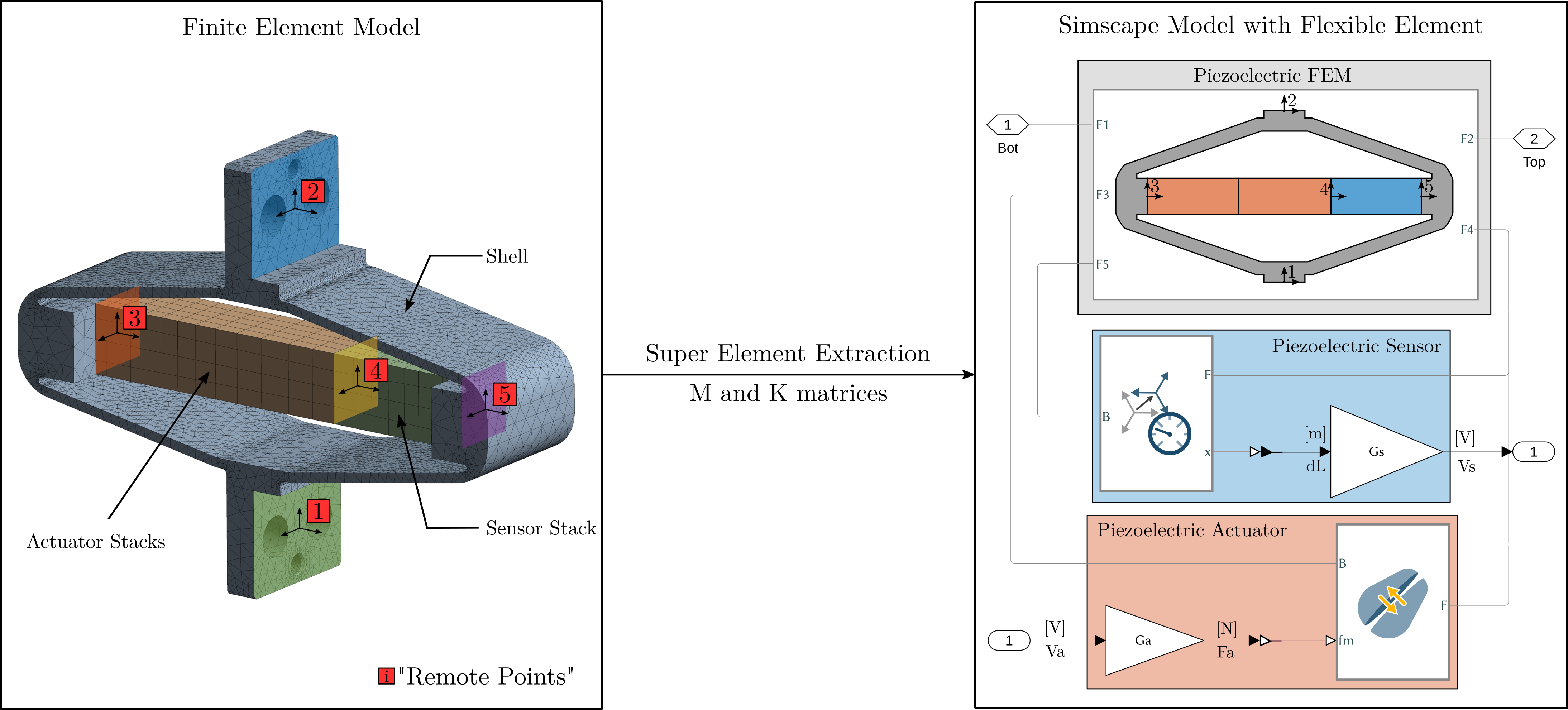
This procedure is illustrated in Figure ref:fig:test_apa_super_element_simscape.
Several remote points are defined in the finite element model (here illustrated by colorful planes and numbers from 1 to 5) and are then made accessible in Simscape as shown at the right by the "frames" F1 to F5.
For the APA300ML super element, 5 remote points are defined.
Two remote points (1 and 2) are fixed to the top and bottom mechanical interfaces of the APA300ML and will be used to connect the APA300ML with other mechanical elements.
Two remote points (3 and 4) are located across two piezoelectric stacks and are used to apply internal forces representing the actuator stacks.
Finally, two remote points (4 and 5) are located across the third piezoelectric stack, and will be used to measured the strain of the sensor stack.
Identification of the Actuator and Sensor constants
Once the APA300ML super element is included in the multi-body model, the transfer function from $F_a$ to $d_L$ and $d_e$ can be extracted. The gains $g_a$ and $g_s$ are then tuned such that the gains of the transfer functions match the identified ones. By doing so, $g_s = 4.9\,V/\mu m$ and $g_a = 23.2\,N/V$ are obtained.
%% Identification of the actuator and sensor "constants"
% Initialize the APA as a flexible body with unity "constants"
n_hexapod.actuator = initializeAPA(...
    'type', 'flexible', ...
    'ga', 1, ...
    'gs', 1);

c_granite = 50; % Rought estimation of the damping added by the air bearing

% Identify the dynamics
G_norm = linearize(mdl, io, 0.0, opts);
G_norm.InputName  = {'u'};
G_norm.OutputName = {'Vs', 'de'};

% Load Identification Data to estimate the two gains
load('meas_apa_frf.mat', 'f', 'Ts', 'enc_frf', 'iff_frf', 'apa_nums');

% Actuator Constant in [N/V]
ga = -mean(abs(enc_frf(f>10 & f<20)))./dcgain(G_norm('de', 'u'));

% Sensor Constant in [V/m]
gs = -mean(abs(iff_frf(f>400 & f<500)))./(ga*abs(squeeze(freqresp(G_norm('Vs', 'u'), 1e3, 'Hz'))));
Comparison of the obtained dynamics
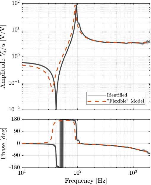
The obtained dynamics using the super element with the tuned "sensor sensitivity" and "actuator sensitivity" are compared with the experimentally identified frequency response functions in Figure ref:fig:test_apa_super_element_comp_frf. A good match between the model and the experimental results was observed. It is however surprising that the model is "softer" than the measured system, as finite element models usually overestimate the stiffness (see Section ref:ssec:test_apa_spurious_resonances for possible explanations).
Using this simple test bench, it can be concluded that the super element model of the APA300ML captures the axial dynamics of the actuator (the actuator stacks, the force sensor stack as well as the shell used as a mechanical lever).
%% Idenfify the dynamics of the Simscape model with correct actuator and sensor "constants"
% Initialize the APA
n_hexapod.actuator = initializeAPA(...
    'type', 'flexible', ...
    'ga',   23.2, ... % Actuator sensitivity [N/V]
    'gs',   -4.9e6);    % Sensor sensitivity [V/m]

% Identify with updated constants
G_flex = exp(-Ts*s)*linearize(mdl, io, 0.0, opts);
G_flex.InputName  = {'u'};
G_flex.OutputName = {'Vs', 'de'};
Conclusion
<<sec:test_apa_conclusion>>
In this study, the amplified piezoelectric actuators "APA300ML" have been characterized to ensure that they fulfill all the requirements determined during the detailed design phase.
Geometrical features such as the flatness of its interfaces, electrical capacitance, and achievable strokes were measured in Section ref:sec:test_apa_basic_meas. These simple measurements allowed for the early detection of a manufacturing defect in one of the APA300ML.
Then in Section ref:sec:test_apa_dynamics, using a dedicated test bench, the dynamics of all the APA300ML were measured and were found to all match very well (Figure ref:fig:test_apa_frf_dynamics). This consistency indicates good manufacturing tolerances, facilitating the modeling and control of the nano-hexapod. Although a non-minimum zero was identified in the transfer function from $u$ to $V_s$ (Figure ref:fig:test_apa_non_minimum_phase), it was found not to be problematic because a large amount of damping could be added using the integral force feedback strategy (Figure ref:fig:test_apa_iff).
Then, two different models were used to represent the APA300ML dynamics. In Section ref:sec:test_apa_model_2dof, a simple two degrees-of-freedom mass-spring-damper model was presented and tuned based on the measured dynamics. After following a tuning procedure, the model dynamics was shown to match very well with the experiment. However, this model only represents the axial dynamics of the actuators, assuming infinite stiffness in other directions.
In Section ref:sec:test_apa_model_flexible, a super element extracted from a finite element model was used to model the APA300ML. Here, the super element represents the dynamics of the APA300ML in all directions. However, only the axial dynamics could be compared with the experimental results, yielding a good match. The benefit of employing this model over the two degrees-of-freedom model is not immediately apparent due to its increased complexity and the larger number of model states involved. Nonetheless, the super element model's value will become clear in subsequent sections, when its capacity to accurately model the APA300ML's flexibility across various directions will be important.
Bibliography ignore
Glossary ignore
Footnotes
6PD200 from PiezoDrive. The gain is $20\,V/V$
5The DAC used is the one included in the IO131 card sold by Speedgoat. It has an output range of $\pm 10\,V$ and 16-bits resolution
13Ansys\textsuperscript{\textregistered} was used
11The transfer function fitting was computed using the vectfit3 routine, see cite:&gustavsen99_ration_approx_frequen_domain_respon
10Frequency of the sinusoidal wave is $1\,\text{Hz}$
9Renishaw Vionic, resolution of $2.5\,nm$
8Kistler 9722A
7Polytec controller 3001 with sensor heads OFV512
12Note that this is not completely correct as it was shown in Section ref:ssec:test_apa_stiffness that the electrical boundaries of the piezoelectric stack impacts its stiffness and that the sensor stack is almost open-circuited while the actuator stacks are almost short-circuited.
2The Matlab fminsearch command is used to fit the plane
1Heidenhain MT25, specified accuracy of $\pm 0.5\,\mu m$
4Millimar 1318 probe, specified linearity better than $1\,\mu m$
3LCR-819 from Gwinstek, with a specified accuracy of $0.05\%$. The measured frequency is set at $1\,\text{kHz}$
