phd-simscape-nass/simscape-nass.org

Simscape Model - Nano Active Stabilization System

• Introduction
• Control Kinematics
  • Introduction
  • Micro Station Kinematics
  • Computation of the sample's pose error
  • Position error in the frame of the struts
  • Control Architecture - Summary
• Decentralized Active Damping
  • Introduction
  • IFF Plant
  • Controller Design
• Centralized Active Vibration Control
  • Introduction
  • HAC Plant
  • Effect of Nano-Hexapod Stiffness on System Dynamics
  • Controller design
  • Tomography experiment
• Conclusion
• Bibliography

Introduction

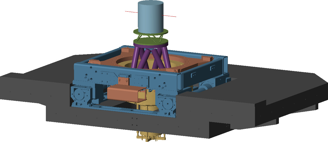
The preceding chapters have established crucial foundational elements for the development of the Nano Active Stabilization System (NASS). The uniaxial model study demonstrated that very stiff nano-hexapod configurations should be avoided due to their high coupling with the micro-station dynamics. A rotating three-degree-of-freedom model revealed that soft nano-hexapod designs prove unsuitable due to gyroscopic effect induced by the spindle rotation. To further improve the model accuracy, a multi-body model of the micro-station was developed, which was carefully tuned using experimental modal analysis. Furthermore, a multi-body model of the nano-hexapod was created, that can then be seamlessly integrated with the micro-station model, as illustrated in Figure ref:fig:nass_simscape_model.

Building upon these foundations, this chapter presents the validation of the NASS concept. The investigation begins with the previously established nano-hexapod model with actuator stiffness $k_a = 1\,N/\mu m$. A thorough examination of the control kinematics is presented in Section ref:sec:nass_kinematics, detailing how both external metrology and nano-hexapod internal sensors are used in the control architecture. The control strategy is then implemented in two steps: first, the decentralized IFF is used for active damping (Section ref:sec:nass_active_damping), then a High Authority Control is develop to stabilize the sample's position in a large bandwidth (Section ref:sec:nass_hac).

The robustness of the proposed control scheme was evaluated under various operational conditions. Particular attention was paid to system performance under changing payload masses and varying spindle rotational velocities.

This chapter concludes the conceptual design phase, with the simulation of tomography experiments providing strong evidence for the viability of the proposed NASS architecture.

Control Kinematics

<<sec:nass_kinematics>>

Introduction   ignore

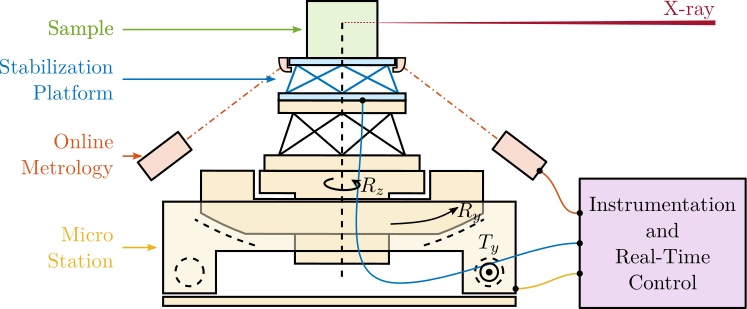
Figure ref:fig:nass_concept_schematic presents a schematic overview of the NASS. This section focuses on the components of the "Instrumentation and Real-Time Control" block.

As established in the previous section on Stewart platforms, the proposed control strategy combines Decentralized Integral Force Feedback with a High Authority Controller performed in the frame of the struts.

For the Nano Active Stabilization System, computing the positioning errors in the frame of the struts involves three key steps. First, desired sample pose with respect to a fixed reference frame is computed using the micro-station kinematics as detailed in Section ref:ssec:nass_ustation_kinematics. This fixed frame is located at the X-ray beam focal point, as it is where the point of interest needs to be positioned. Second, it measures the actual sample pose relative to the same fix frame, described in Section ref:ssec:nass_sample_pose_error. Finally, it determines the sample pose error and maps these errors to the nano-hexapod struts, as explained in Section ref:ssec:nass_error_struts.

The complete control architecture is described in Section ref:ssec:nass_control_architecture.

Micro Station Kinematics

<<ssec:nass_ustation_kinematics>>

The micro-station kinematics enables the computation of the desired sample pose from the reference signals of each micro-station stage. These reference signals consist of the desired lateral position $r_{D_y}$, tilt angle $r_{R_y}$, and spindle angle $r_{R_z}$. The micro-hexapod pose is defined by six parameters: three translations ($r_{D_{\mu x}}$, $r_{D_{\mu y}}$, $r_{D_{\mu z}}$) and three rotations ($r_{\theta_{\mu x}}$, $r_{\theta_{\mu y}}$, $r_{\theta_{\mu z}}$).

Using these reference signals, the desired sample position relative to the fixed frame is expressed through the homogeneous transformation matrix $\bm{T}_{\mu\text{-station}}$, as defined in equation eqref:eq:nass_sample_ref.

\begin{equation}\label{eq:nass_sample_ref} \bm{T}_{μ\text{-station}} = \bm{T}_{D_y} ⋅ \bm{T}_{R_y} ⋅ \bm{T}_{R_z} ⋅ \bm{T}_{μ\text{-hexapod}}

\end{equation}

\begin{equation}\label{eq:nass_ustation_matrices}

\begin{align} \bm{T}_{D_y} &= \begin{bmatrix} 1 & 0 & 0 & 0 \\ 0 & 1 & 0 & r_{D_y} \\ 0 & 0 & 1 & 0 \\ 0 & 0 & 0 & 1 \end{bmatrix} \quad \bm{T}_{\mu\text{-hexapod}} = \left[ \begin{array}{ccc|c} & & & r_{D_{\mu x}} \\ & \bm{R}_x(r_{\theta_{\mu x}}) \bm{R}_y(r_{\theta_{\mu y}}) \bm{R}_{z}(r_{\theta_{\mu z}}) & & r_{D_{\mu y}} \\ & & & r_{D_{\mu z}} \cr \hline 0 & 0 & 0 & 1 \end{array} \right] \\ \bm{T}_{R_z} &= \begin{bmatrix} \cos(r_{R_z}) & -\sin(r_{R_z}) & 0 & 0 \\ \sin(r_{R_z}) & \cos(r_{R_z}) & 0 & 0 \\ 0 & 0 & 1 & 0 \\ 0 & 0 & 0 & 1 \end{bmatrix} \quad \bm{T}_{R_y} = \begin{bmatrix} \cos(r_{R_y}) & 0 & \sin(r_{R_y}) & 0 \\ 0 & 1 & 0 & 0 \\ -\sin(r_{R_y}) & 0 & \cos(r_{R_y}) & 0 \\ 0 & 0 & 0 & 1 \end{bmatrix} \end{align}

\end{equation}

Computation of the sample's pose error

<<ssec:nass_sample_pose_error>>

The external metrology system measures the sample position relative to the fixed granite. Due to the system's symmetry, this metrology provides measurements for five degrees of freedom: three translations ($D_x$, $D_y$, $D_z$) and two rotations ($R_x$, $R_y$).

The sixth degree of freedom ($R_z$) is still required to compute the errors in the frame of the nano-hexapod struts (i.e. to compute the nano-hexapod inverse kinematics). This $R_z$ rotation is estimated by combining measurements from the spindle encoder and the nano-hexapod's internal metrology, which consists of relative motion sensors in each strut (note that the micro-hexapod is not used for $R_z$ rotation, and is therefore ignore for $R_z$ estimation).

The measured sample pose is represented by the homogeneous transformation matrix $\bm{T}_{\text{sample}}$, as shown in equation eqref:eq:nass_sample_pose.

\begin{equation}\label{eq:nass_sample_pose} \bm{T}_{\text{sample}} = ≤ft[ \begin{array}{ccc|c} & & & D_{x} \\ & \bm{R}_x(R_{x}) \bm{R}_y(R_{y}) \bm{R}_{z}(R_{z}) & & D_{y} \\ & & & D_{z} \cr \hline 0 & 0 & 0 & 1 \end{array} \right]

\end{equation}

Position error in the frame of the struts

<<ssec:nass_error_struts>>

The homogeneous transformation formalism enables straightforward computation of the sample position error. This computation involves the previously computed homogeneous $4 \times 4$ matrices: $\bm{T}_{\mu\text{-station}}$ representing the desired pose, and $\bm{T}_{\text{sample}}$ representing the measured pose. Their combination yields $\bm{T}_{\text{error}}$, which expresses the position error of the sample in the frame of the rotating nano-hexapod, as shown in equation eqref:eq:nass_transformation_error.

\begin{equation}\label{eq:nass_transformation_error} \bm{T}_{\text{error}} = \bm{T}_{μ\text{-station}}^-1 ⋅ \bm{T}_{\text{sample}}

\end{equation}

The known structure of the homogeneous transformation matrix facilitates efficient real-time inverse computation. From $\bm{T}_{\text{error}}$, the position and orientation errors $\bm{\epsilon}_{\mathcal{X}} = [\epsilon_{D_x},\ \epsilon_{D_y},\ \epsilon_{D_z},\ \epsilon_{R_x},\ \epsilon_{R_y},\ \epsilon_{R_z}]$ of the sample are extracted using equation eqref:eq:nass_compute_errors:

\begin{equation}\label{eq:nass_compute_errors}

\begin{align} \epsilon_{D_x} & = \bm{T}_{\text{error}}(1,4) \\ \epsilon_{D_y} & = \bm{T}_{\text{error}}(2,4) \\ \epsilon_{D_z} & = \bm{T}_{\text{error}}(3,4) \\ \epsilon_{R_y} & = \text{atan2}(\bm{T}_{\text{error}}(1,3), \sqrt{\bm{T}_{\text{error}}(1,1)^2 + \bm{T}_{\text{error}}(1,2)^2}) \\ \epsilon_{R_x} & = \text{atan2}(-\bm{T}_{\text{error}}(2,3)/\cos(\epsilon_{R_y}), \bm{T}_{\text{error}}(3,3)/\cos(\epsilon_{R_y})) \\ \epsilon_{R_z} & = \text{atan2}(-\bm{T}_{\text{error}}(1,2)/\cos(\epsilon_{R_y}), \bm{T}_{\text{error}}(1,1)/\cos(\epsilon_{R_y})) \\ \end{align}

\end{equation}

Finally, these errors are mapped to the strut space using the nano-hexapod Jacobian matrix eqref:eq:nass_inverse_kinematics.

\begin{equation}\label{eq:nass_inverse_kinematics} \bm{ε}_{\mathcal{L}} = \bm{J} ⋅ \bm{ε}_{\mathcal{X}}

\end{equation}

Control Architecture - Summary

<<ssec:nass_control_architecture>>

The complete control architecture is summarized in Figure ref:fig:nass_control_architecture. The sample pose is measured using external metrology for five degrees of freedom, while the sixth degree of freedom (Rz) is estimated by combining measurements from the nano-hexapod encoders and spindle encoder.

The sample reference pose is determined by the reference signals of the translation stage, tilt stage, spindle, and micro-hexapod. The position error computation follows a two-step process: first, homogeneous transformation matrices are used to determine the error in the nano-hexapod frame. Then, the Jacobian matrix $\bm{J}$ maps these errors to individual strut coordinates.

For control purposes, force sensors mounted on each strut are used in a decentralized manner for active damping, as detailed in Section ref:sec:nass_active_damping. Then, the high authority controller uses the computed errors in the frame of the struts to provides real-time stabilization of the sample position (Section ref:sec:nass_hac).

\begin{tikzpicture}
  % Blocs
  \node[block={2.0cm}{1.0cm}, fill=colorblue!20!white] (metrology) {Metrology};
  \node[block={2.0cm}{2.0cm}, below=0.1 of metrology, align=center, fill=colorblue!20!white] (nhexa) {Nano\\Hexapod};
  \node[block={3.0cm}{1.5cm}, below=0.1 of nhexa, align=center, fill=colorblue!20!white] (ustation) {Micro\\Station};

  \coordinate[] (inputf)  at ($(nhexa.south west)!0.5!(nhexa.north west)$);
  \coordinate[] (outputfn) at ($(nhexa.south east)!0.3!(nhexa.north east)$);
  \coordinate[] (outputde) at ($(nhexa.south east)!0.7!(nhexa.north east)$);

  \coordinate[] (outputDy) at ($(ustation.south east)!0.1!(ustation.north east)$);
  \coordinate[] (outputRy) at ($(ustation.south east)!0.5!(ustation.north east)$);
  \coordinate[] (outputRz) at ($(ustation.south east)!0.9!(ustation.north east)$);

  \node[block={1.0cm}{1.0cm}, right=0.5 of outputde, fill=colorred!20!white] (Rz_kinematics) {$\bm{J}_{R_z}^{-1}$};
  \node[block={2.0cm}{2.0cm}, right=2.2 of ustation, align=center, fill=colorred!20!white] (ustation_kinematics) {Compute\\Reference\\Position};
  \node[block={2.0cm}{2.0cm}, right=0.8 of ustation_kinematics, align=center, fill=colorred!20!white] (compute_error) {Compute\\Error\\Position};
  \node[block={2.0cm}{2.0cm}, above=0.8 of compute_error, align=center, fill=colorred!20!white] (compute_pos) {Compute\\Sample\\Position};
  \node[block={1.0cm}{1.0cm}, right=0.8 of compute_error, fill=colorred!20!white] (hexa_jacobian) {$\bm{J}$};

  \coordinate[] (inputMetrology) at ($(compute_error.north east)!0.3!(compute_error.north west)$);
  \coordinate[] (inputRz) at ($(compute_error.north east)!0.7!(compute_error.north west)$);

  \node[addb={+}{}{}{}{}, right=0.4 of Rz_kinematics, fill=colorred!20!white] (addRz) {};
  \draw[->] (Rz_kinematics.east) -- (addRz.west);
  \draw[->] (outputRz-|addRz)node[branch]{} -- (addRz.south);

  \draw[->] (outputDy) node[above right]{$r_{D_y}$} -- (outputDy-|ustation_kinematics.west);
  \draw[->] (outputRy) node[above right]{$r_{R_y}$} -- (outputRy-|ustation_kinematics.west);
  \draw[->] (outputRz) node[above right]{$r_{R_z}$} -- (outputRz-|ustation_kinematics.west);

  \draw[->] (metrology.east)node[above right]{$[D_x,\,D_y,\,D_z,\,R_x,\,R_y]$} -- (compute_pos.west|-metrology);
  \draw[->] (addRz.east)node[above right]{$R_z$} -- (compute_pos.west|-addRz);
  \draw[->] (compute_pos.south)node -- (compute_error.north)node[above right]{$\bm{y}_{\mathcal{X}}$};

  \draw[->] (outputde) -- (Rz_kinematics.west) node[above left]{$\bm{\mathcal{L}}$};
  \draw[->] (ustation_kinematics.east) -- (compute_error.west) node[above left]{$\bm{r}_{\mathcal{X}}$};
  \draw[->] (compute_error.east) -- (hexa_jacobian.west) node[above left]{$\bm{\epsilon\mathcal{X}}$};
  \draw[->] (hexa_jacobian.east) -- ++(1.8, 0) node[above left]{$\bm{\epsilon\mathcal{L}}$};

  \draw[->] (outputfn) -- ($(outputfn-|hexa_jacobian.east) + (1.0, 0)$)coordinate(fn) node[above left]{$\bm{f}_n$};

  \begin{scope}[on background layer]
    \node[fit={(metrology.north-|ustation.west) (hexa_jacobian.east|-compute_error.south)}, fill=black!10!white, draw, dashed, inner sep=4pt] (plant) {};
    \node[anchor={north east}] at (plant.north east){$\text{Plant}$};
  \end{scope}

  \node[block, above=0.2 of plant, fill=coloryellow!20!white] (Kiff) {$\bm{K}_{\text{IFF}}$};
  \draw[->] ($(fn)-(0.6,0)$)node[branch]{} |- (Kiff.east);

  \node[addb={+}{}{}{}{}, left=0.8 of inputf] (addf) {};
  \draw[->] (Kiff.west) -| (addf.north);

  \begin{scope}[on background layer]
    \node[fit={(plant.south-|fn) (addf.west|-Kiff.north)}, fill=black!20!white, draw, dashed, inner sep=4pt] (damped_plant) {};
    \node[anchor={north east}] at (damped_plant.north east){$\text{Damped Plant}$};
  \end{scope}

  \begin{scope}[on background layer]
    \node[fit={(metrology.north-|ustation.west) (hexa_jacobian.east|-compute_error.south)}, fill=black!10!white, draw, dashed, inner sep=4pt] (plant) {};
    \node[anchor={north east}] at (plant.north east){$\text{Plant}$};
  \end{scope}

  \node[block, left=0.8 of addf, fill=colorgreen!20!white] (Khac) {$\bm{K}_{\text{HAC}}$};
  \draw[->] ($(hexa_jacobian.east)+(1.4,0)$)node[branch]{} |- ($(Khac.west)+(-0.4, -3.4)$) |- (Khac.west);
  \draw[->] (Khac.east) -- node[midway, above]{$\bm{f}^{\prime}$} (addf.west);
  \draw[->] (addf.east) -- (inputf) node[above left]{$\bm{f}$};
\end{tikzpicture}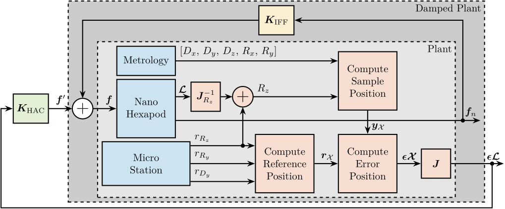

Decentralized Active Damping

<<sec:nass_active_damping>>

Introduction   ignore

Building on the uniaxial model study, this section implements decentralized Integral Force Feedback (IFF) as the first component of the HAC-LAC strategy. The springs in parallel to the force sensors were used to guarantee the control robustness, as observed with the 3DoF rotating model. The objective here is to design a decentralized IFF controller that provides good damping of the nano-hexapod modes across payload masses ranging from $1$ to $50\,\text{kg}$ and rotational velocity up to $360\,\text{deg/s}$. The payloads used for validation have a cylindrical shape with 250 mm height and with masses of 1 kg, 25 kg, and 50 kg.

IFF Plant

<<ssec:nass_active_damping_plant>>

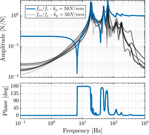
Transfer functions from actuator forces $f_i$ to force sensor measurements $f_{mi}$ are computed using the multi-body model. Figure ref:fig:nass_iff_plant_effect_kp examines how parallel stiffness affects plant dynamics, with identification performed at maximum spindle velocity $\Omega_z = 360\,\text{deg/s}$ and with a payload mass of 25 kg.

Without parallel stiffness (Figure ref:fig:nass_iff_plant_no_kp), the dynamics exhibit non-minimum phase zeros at low frequency, confirming predictions from the three-degree-of-freedom rotating model. Adding parallel stiffness (Figure ref:fig:nass_iff_plant_kp) transforms these into minimum phase complex conjugate zeros, enabling unconditionally stable decentralized IFF implementation.

Although both cases show significant coupling around the resonances, stability is guaranteed by the collocated arrangement of the actuators and sensors cite:&preumont08_trans_zeros_struc_contr_with.

%% Identify the IFF plant dynamics using the Simscape model

% Initialize each Simscape model elements
initializeGround();
initializeGranite();
initializeTy();
initializeRy();
initializeRz();
initializeMicroHexapod();
initializeSimplifiedNanoHexapod();

% Initial Simscape Configuration
initializeSimscapeConfiguration('gravity', false);
initializeDisturbances('enable', false);
initializeLoggingConfiguration('log', 'none');
initializeController('type', 'open-loop');
initializeReferences();

% Input/Output definition
clear io; io_i = 1;
io(io_i) = linio([mdl, '/Controller'], 1, 'openinput');             io_i = io_i + 1; % Actuator Inputs [N]
io(io_i) = linio([mdl, '/NASS'],       3, 'openoutput', [], 'fn');  io_i = io_i + 1; % Force Sensors [N]

% Identify for multi payload masses (no rotation)
initializeReferences(); % No Spindle Rotation
% 1kg Sample
initializeSample('type', 'cylindrical', 'm', 1);
G_iff_m1 = linearize(mdl, io);
G_iff_m1.InputName  = {'f1',  'f2',  'f3',  'f4',  'f5',  'f6'};
G_iff_m1.OutputName = {'fn1', 'fn2', 'fn3', 'fn4', 'fn5', 'fn6'};

% 25kg Sample
initializeSample('type', 'cylindrical', 'm', 25);
G_iff_m25 = linearize(mdl, io);
G_iff_m25.InputName  = {'f1',  'f2',  'f3',  'f4',  'f5',  'f6'};
G_iff_m25.OutputName = {'fn1', 'fn2', 'fn3', 'fn4', 'fn5', 'fn6'};

% 50kg Sample
initializeSample('type', 'cylindrical', 'm', 50);
G_iff_m50 = linearize(mdl, io);
G_iff_m50.InputName  = {'f1',  'f2',  'f3',  'f4',  'f5',  'f6'};
G_iff_m50.OutputName = {'fn1', 'fn2', 'fn3', 'fn4', 'fn5', 'fn6'};

% Effect of Rotation
initializeReferences(...
    'Rz_type', 'rotating', ...
    'Rz_period', 1); % 360 deg/s
initializeSample('type', 'cylindrical', 'm', 25);
G_iff_m25_Rz = linearize(mdl, io, 0.1);
G_iff_m25_Rz.InputName  = {'f1',  'f2',  'f3',  'f4',  'f5',  'f6'};
G_iff_m25_Rz.OutputName = {'fn1', 'fn2', 'fn3', 'fn4', 'fn5', 'fn6'};

% Effect of Rotation - No added parallel stiffness
initializeSimplifiedNanoHexapod('actuator_kp', 0);
initializeReferences(...
    'Rz_type', 'rotating', ...
    'Rz_period', 1); % 360 deg/s
initializeSample('type', 'cylindrical', 'm', 25);
G_iff_m25_Rz_no_kp = linearize(mdl, io, 0.1);
G_iff_m25_Rz_no_kp.InputName  = {'f1',  'f2',  'f3',  'f4',  'f5',  'f6'};
G_iff_m25_Rz_no_kp.OutputName = {'fn1', 'fn2', 'fn3', 'fn4', 'fn5', 'fn6'};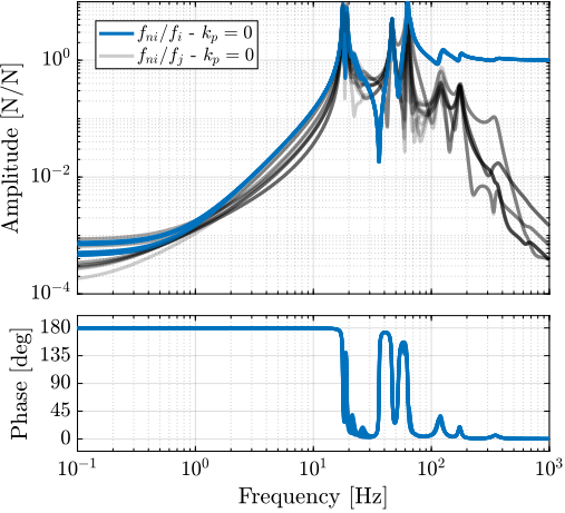

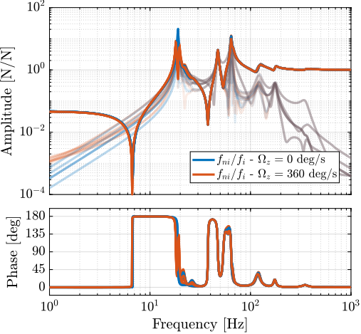
The effect of rotation, as shown in Figure ref:fig:nass_iff_plant_effect_rotation, is negligible as the actuator stiffness ($k_a = 1\,N/\mu m$) is large compared to the negative stiffness induced by gyroscopic effects (estimated from the 3DoF rotating model).

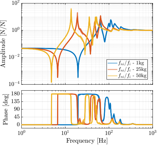
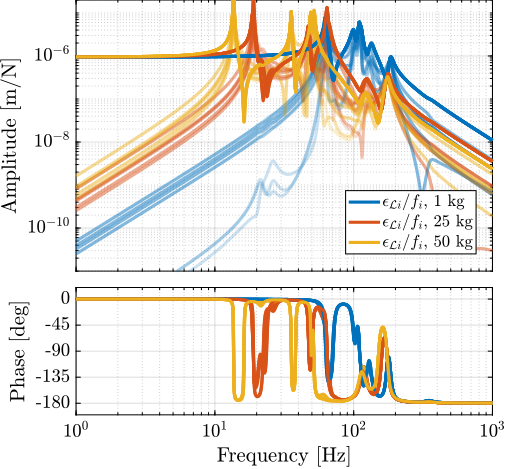
Figure ref:fig:nass_iff_plant_effect_payload illustrate the effect of payload mass on the plant dynamics. The poles and zeros shift in frequency as the payload mass varies. However, their alternating pattern is preserved, which ensures the phase remains bounded between 0 and 180 degrees, thus maintaining robust stability properties.

Controller Design

<<ssec:nass_active_damping_control>>

The previous analysis using the 3DoF rotating model showed that decentralized Integral Force Feedback (IFF) with pure integrators is unstable due to the gyroscopic effects caused by spindle rotation. This finding was also confirmed with the multi-body model of the NASS: the system was unstable when using pure integrators and without parallel stiffness.

This instability can be mitigated by introducing sufficient stiffness in parallel with the force sensors. However, as illustrated in Figure ref:fig:nass_iff_plant_kp, adding parallel stiffness increases the low frequency gain. Using pure integrators would result in high loop gain at low frequencies, adversely affecting the damped plant dynamics, which is undesirable. To resolve this issue, a second-order high-pass filter is introduced to limit the low frequency gain, as shown in Equation eqref:eq:nass_kiff.

\begin{equation}\label{eq:nass_kiff} \bm{K}_{\text{IFF}}(s) = g ⋅ \begin{bmatrix} K_{\text{IFF}}(s) & & 0 \\ & \ddots & \\ 0 & & K_{\text{IFF}}(s) \end{bmatrix}, \quad K_{\text{IFF}}(s) = \frac{1}{s} ⋅ \frac{\frac{s^2}{ω_z^2}}{\frac{s^2}{ω_z^2} + 2 ξ_z \frac{s}{ω_z} + 1}

\end{equation}

The cut-off frequency of the second-order high-pass filter was tuned to be below the frequency of the complex conjugate zero for the highest mass, which is at $5\,\text{Hz}$. The overall gain was then increased to obtain a large loop gain around the resonances to be damped, as illustrated in Figure ref:fig:nass_iff_loop_gain.

%% Verify that parallel stiffness permits to have a stable plant
Kiff_pure_int = -200/s*eye(6);
isstable(feedback(G_iff_m25_Rz,       Kiff_pure_int, 1))
isstable(feedback(G_iff_m25_Rz_no_kp, Kiff_pure_int, 1))

%% IFF Controller Design
% Second order high pass filter
wz = 2*pi*2;
xiz = 0.7;
Ghpf = (s^2/wz^2)/(s^2/wz^2 + 2*xiz*s/wz + 1);

Kiff = -200 * ...              % Gain
       1/(0.01*2*pi + s) * ... % LPF: provides integral action
       Ghpf * ...              % 2nd order HPF (limit low frequency gain)
       eye(6);                 % Diagonal 6x6 controller (i.e. decentralized)

Kiff.InputName = {'fm1', 'fm2', 'fm3', 'fm4', 'fm5', 'fm6'};
Kiff.OutputName = {'f1', 'f2', 'f3', 'f4', 'f5', 'f6'};

% The designed IFF controller is saved
save('./mat/nass_K_iff.mat', 'Kiff');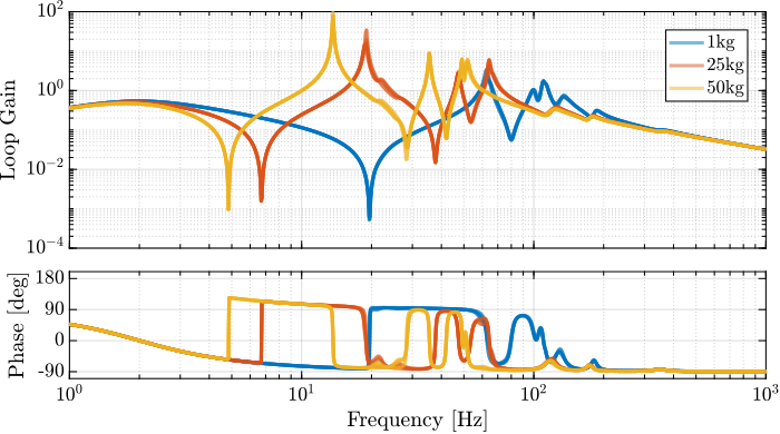

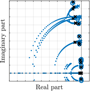
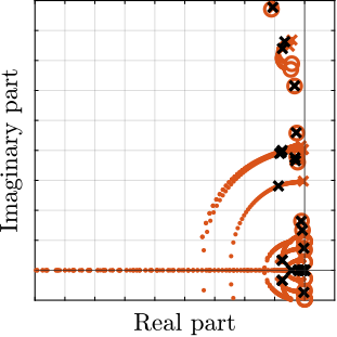
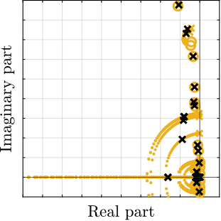
To verify stability, the root loci for the three payload configurations were computed, as shown in Figure ref:fig:nass_iff_root_locus. The results demonstrate that the closed-loop poles remain within the left-half plane, indicating the robust stability of the applied decentralized IFF.

Centralized Active Vibration Control

<<sec:nass_hac>>

Introduction   ignore

The implementation of high-bandwidth position control for the nano-hexapod presents several technical challenges. The plant dynamics exhibit complex behavior influenced by multiple factors, including payload mass, rotational velocity, and the mechanical coupling between the nano-hexapod and the micro-station. This section presents the development and validation of a centralized control strategy designed to achieve precise sample positioning during high-speed tomography experiments.

First, a comprehensive analysis of the plant dynamics is presented in Section ref:ssec:nass_hac_plant, examining the effects of spindle rotation, payload mass variation, and the implementation of Integral Force Feedback (IFF). Section ref:ssec:nass_hac_stiffness validates previous modeling predictions that both overly stiff and compliant nano-hexapod configurations lead to degraded performance. Building upon these findings, Section ref:ssec:nass_hac_controller presents the design of a robust high-authority controller that maintains stability across varying payload masses while achieving the desired control bandwidth.

The performance of the developed control strategy was validated through simulations of tomography experiments in Section ref:ssec:nass_hac_tomography. These simulations incorporated realistic disturbance sources and were used to evaluate the system performance against the stringent positioning requirements imposed by future beamline specifications. Particular attention was paid to the system's behavior under maximum rotational velocity conditions and its ability to accommodate varying payload masses, demonstrating the practical viability of the proposed control approach.

HAC Plant

<<ssec:nass_hac_plant>>

The plant dynamics from force inputs $\bm{f}$ to the strut errors $\bm{\epsilon}_{\mathcal{L}}$ were first extracted from the multi-body model without the implementation of the decentralized IFF. The influence of spindle rotation on plant dynamics was investigated, and the results are presented in Figure ref:fig:nass_undamped_plant_effect_Wz. While rotational motion introduces coupling effects at low frequencies, these effects remain minimal at operational velocities, owing to the high stiffness characteristics of the nano-hexapod assembly.

Payload mass emerged as a significant parameter affecting system behavior, as illustrated in Figure ref:fig:nass_undamped_plant_effect_mass. As expected, increasing the payload mass decreased the resonance frequencies while amplifying coupling at low frequency. These mass-dependent dynamic changes present considerable challenges for control system design, particularly for configurations with high payload masses.

Additional operational parameters were systematically evaluated, including the $R_y$ tilt angle, $R_z$ spindle position, and micro-hexapod position. These factors were found to exert negligible influence on the plant dynamics, which can be attributed to the effective mechanical decoupling achieved between the plant and micro-station dynamics. This decoupling characteristic ensures consistent performance across various operational configurations. This also validates the developed control kinematics.

%% Identify the IFF plant dynamics using the Simscape model

% Initialize each Simscape model elements
initializeGround();
initializeGranite();
initializeTy();
initializeRy();
initializeRz();
initializeMicroHexapod();
initializeSimplifiedNanoHexapod();
initializeSample('type', 'cylindrical', 'm', 1);

% Initial Simscape Configuration
initializeSimscapeConfiguration('gravity', false);
initializeDisturbances('enable', false);
initializeLoggingConfiguration('log', 'none');
initializeController('type', 'open-loop');
initializeReferences();

% Input/Output definition
clear io; io_i = 1;
io(io_i) = linio([mdl, '/Controller'],     1, 'input');                  io_i = io_i + 1; % Actuator Inputs [N]
io(io_i) = linio([mdl, '/Tracking Error'], 1, 'openoutput', [], 'EdL');  io_i = io_i + 1; % Strut errors [m]

% Identify HAC Plant without using IFF
initializeSample('type', 'cylindrical', 'm', 1);
G_m1 = linearize(mdl, io);
G_m1.InputName  = {'f1', 'f2', 'f3', 'f4', 'f5', 'f6'};
G_m1.OutputName = {'l1', 'l2', 'l3', 'l4', 'l5', 'l6'};

initializeSample('type', 'cylindrical', 'm', 25);
G_m25 = linearize(mdl, io);
G_m25.InputName  = {'f1', 'f2', 'f3', 'f4', 'f5', 'f6'};
G_m25.OutputName = {'l1', 'l2', 'l3', 'l4', 'l5', 'l6'};

initializeSample('type', 'cylindrical', 'm', 50);
G_m50 = linearize(mdl, io);
G_m50.InputName  = {'f1', 'f2', 'f3', 'f4', 'f5', 'f6'};
G_m50.OutputName = {'l1', 'l2', 'l3', 'l4', 'l5', 'l6'};

% Effect of Rotation
initializeSample('type', 'cylindrical', 'm', 1);
initializeReferences(...
    'Rz_type', 'rotating', ...
    'Rz_period', 1); % 360 deg/s

G_m1_Rz = linearize(mdl, io, 0.1);
G_m1_Rz.InputName  = {'f1',  'f2',  'f3',  'f4',  'f5',  'f6'};
G_m1_Rz.OutputName = {'l1', 'l2', 'l3', 'l4', 'l5', 'l6'};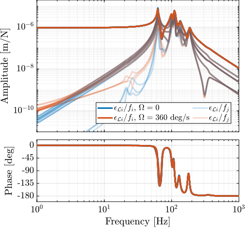

The Decentralized Integral Force Feedback was implemented in the multi-body model, and transfer functions from force inputs $\bm{f}^\prime$ of the damped plant to the strut errors $\bm{\epsilon}_{\mathcal{L}}$ were extracted from this model.

The effectiveness of the IFF implementation was first evaluated with a $1\,\text{kg}$ payload, as demonstrated in Figure ref:fig:nass_comp_undamped_damped_plant_m1. The results indicate successful damping of the nano-hexapod resonance modes, although a minor increase in low-frequency coupling was observed. This trade-off was considered acceptable, given the overall improvement in system behavior.

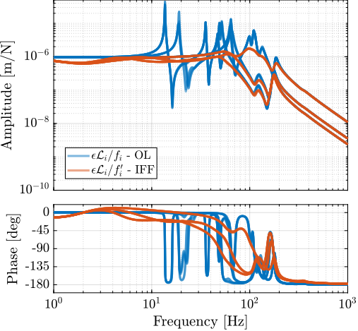
The benefits of IFF implementation were further assessed across the full range of payload configurations, and the results are presented in Figure ref:fig:nass_hac_plants. For all tested payloads ($1\,\text{kg}$, $25\,\text{kg}$ and $50\,\text{kg}$), the decentralized IFF significantly damped the nano-hexapod modes and therefore simplified the system dynamics. More importantly, in the vicinity of the desired high authority control bandwidth (i.e. between $10\,\text{Hz}$ and $50\,\text{Hz}$), the damped dynamics (shown in red) exhibited minimal gain and phase variations with frequency. For the undamped plants (shown in blue), achieving robust control with bandwidth above 10Hz while maintaining stability across different payload masses would be practically impossible.

%% Identify HAC Plant with IFF
initializeReferences(); % No Spindle Rotation
initializeController('type', 'iff'); % Implemented IFF controller
load('nass_K_iff.mat', 'Kiff'); % Load designed IFF controller

% 1kg payload
initializeSample('type', 'cylindrical', 'm', 1);
G_hac_m1 = linearize(mdl, io);
G_hac_m1.InputName  = {'f1', 'f2', 'f3', 'f4', 'f5', 'f6'};
G_hac_m1.OutputName = {'l1', 'l2', 'l3', 'l4', 'l5', 'l6'};

% 25kg payload
initializeSample('type', 'cylindrical', 'm', 25);
G_hac_m25 = linearize(mdl, io);
G_hac_m25.InputName  = {'f1', 'f2', 'f3', 'f4', 'f5', 'f6'};
G_hac_m25.OutputName = {'l1', 'l2', 'l3', 'l4', 'l5', 'l6'};

% 50kg payload
initializeSample('type', 'cylindrical', 'm', 50);
G_hac_m50 = linearize(mdl, io);
G_hac_m50.InputName  = {'f1', 'f2', 'f3', 'f4', 'f5', 'f6'};
G_hac_m50.OutputName = {'l1', 'l2', 'l3', 'l4', 'l5', 'l6'};

% Check stability
if not(isstable(G_hac_m1) && isstable(G_hac_m25) && isstable(G_hac_m50))
    warning('One of HAC plant is not stable')
end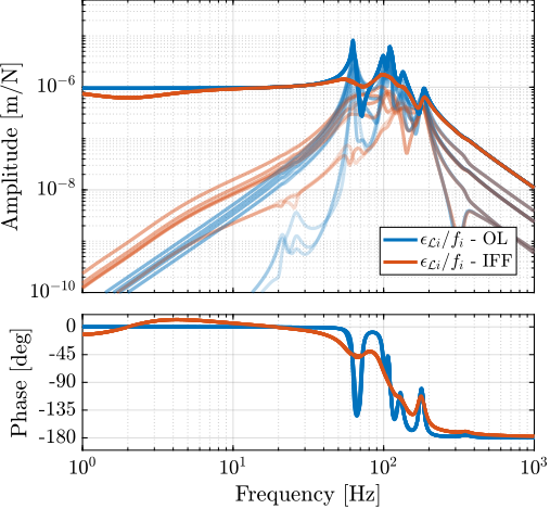

The coupling between the nano-hexapod and the micro-station was evaluated through a comparative analysis of plant dynamics under two mounting conditions. In the first configuration, the nano-hexapod was mounted on an ideally rigid support, while in the second configuration, it was installed on the micro-station with finite compliance.

As illustrated in Figure ref:fig:nass_effect_ustation_compliance, the complex dynamics of the micro-station were found to have little impact on the plant dynamics. The only observable difference manifests as additional alternating poles and zeros above 100Hz, a frequency range sufficiently beyond the control bandwidth to avoid interference with the system performance. This result confirms effective dynamic decoupling between the nano-hexapod and the supporting micro-station structure.

%% Identify plant with "rigid" micro-station
initializeGround('type', 'rigid');
initializeGranite('type', 'rigid');
initializeTy('type', 'rigid');
initializeRy('type', 'rigid');
initializeRz('type', 'rigid');
initializeMicroHexapod('type', 'rigid');
initializeSimplifiedNanoHexapod();
initializeSample('type', 'cylindrical', 'm', 25);

initializeReferences();
initializeController('type', 'open-loop'); % Implemented IFF controller
load('nass_K_iff.mat', 'Kiff'); % Load designed IFF controller

% Input/Output definition
clear io; io_i = 1;
io(io_i) = linio([mdl, '/Controller'],     1, 'input');                  io_i = io_i + 1; % Actuator Inputs [N]
io(io_i) = linio([mdl, '/Tracking Error'], 1, 'openoutput', [], 'EdL');  io_i = io_i + 1; % Strut errors [m]

G_m25_rigid = linearize(mdl, io);
G_m25_rigid.InputName  = {'f1', 'f2', 'f3', 'f4', 'f5', 'f6'};
G_m25_rigid.OutputName = {'l1', 'l2', 'l3', 'l4', 'l5', 'l6'};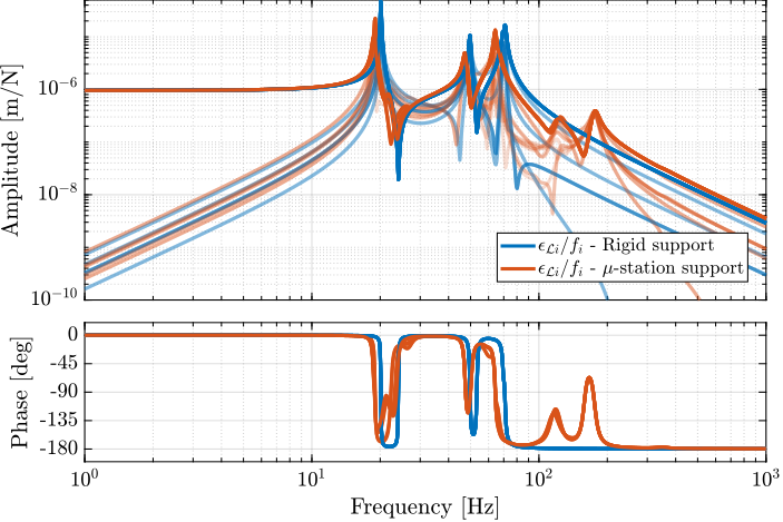

Effect of Nano-Hexapod Stiffness on System Dynamics

<<ssec:nass_hac_stiffness>>

The influence of nano-hexapod stiffness was investigated to validate earlier findings from simplified uniaxial and three-degree-of-freedom (3DoF) models. These models suggest that a moderate stiffness of approximately $1\,N/\mu m$ would provide better performance than either very stiff or very soft configurations.

For the stiff nano-hexapod analysis, a system with an actuator stiffness of $100\,N/\mu m$ was simulated with a $25\,\text{kg}$ payload. The transfer function from $\bm{f}$ to $\bm{\epsilon}_{\mathcal{L}}$ was evaluated under two conditions: mounting on an infinitely rigid base and mounting on the micro-station. As shown in Figure ref:fig:nass_stiff_nano_hexapod_coupling_ustation, significant coupling was observed between the nano-hexapod and micro-station dynamics. This coupling introduces complex behavior that is difficult to model and predict accurately, thus corroborating the predictions of the simplified uniaxial model.

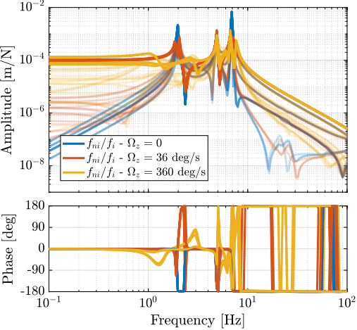
The soft nano-hexapod configuration was evaluated using a stiffness of $0.01\,N/\mu m$ with a $25\,\text{kg}$ payload. The dynamic response was characterized at three rotational velocities: 0, 36, and 360 deg/s. Figure ref:fig:nass_soft_nano_hexapod_effect_Wz demonstrates that rotation substantially affects system dynamics, manifesting as instability at high rotational velocities, increased coupling due to gyroscopic effects, and rotation-dependent resonance frequencies. The current approach of controlling the position in the strut frame is inadequate for soft nano-hexapods; but even shifting control to a frame matching the payload's center of mass would not overcome the substantial coupling and dynamic variations induced by gyroscopic effects.

%% Identify Dynamics with a Stiff nano-hexapod (100N/um)

% Initialize each Simscape model elements
initializeGround();
initializeGranite();
initializeTy();
initializeRy();
initializeRz();
initializeMicroHexapod();
initializeSimplifiedNanoHexapod('actuator_k', 1e8, 'actuator_kp', 0, 'actuator_c', 1e3);
initializeSample('type', 'cylindrical', 'm', 25);

% Initial Simscape Configuration
initializeSimscapeConfiguration('gravity', false);
initializeDisturbances('enable', false);
initializeLoggingConfiguration('log', 'none');
initializeController('type', 'open-loop');
initializeReferences();

% Input/Output definition
clear io; io_i = 1;
io(io_i) = linio([mdl, '/Controller'],     1, 'input');                  io_i = io_i + 1; % Actuator Inputs [N]
io(io_i) = linio([mdl, '/Tracking Error'], 1, 'openoutput', [], 'EdL');  io_i = io_i + 1; % Strut errors [m]

% Identify Plant
G_m25_pz = linearize(mdl, io);
G_m25_pz.InputName  = {'f1', 'f2', 'f3', 'f4', 'f5', 'f6'};
G_m25_pz.OutputName = {'l1', 'l2', 'l3', 'l4', 'l5', 'l6'};

% Compare with Nano-Hexapod alone (rigid micro-station)
initializeGround('type', 'rigid');
initializeGranite('type', 'rigid');
initializeTy('type', 'rigid');
initializeRy('type', 'rigid');
initializeRz('type', 'rigid');
initializeMicroHexapod('type', 'rigid');

% Identify Plant
G_m25_pz_rigid = linearize(mdl, io);
G_m25_pz_rigid.InputName  = {'f1', 'f2', 'f3', 'f4', 'f5', 'f6'};
G_m25_pz_rigid.OutputName = {'l1', 'l2', 'l3', 'l4', 'l5', 'l6'};

%% Identify Dynamics with a Soft nano-hexapod (0.01N/um)
initializeGround();
initializeGranite();
initializeTy();
initializeRy();
initializeRz();
initializeMicroHexapod();
initializeSimplifiedNanoHexapod('actuator_k', 1e4, 'actuator_kp', 0, 'actuator_c', 1);

% Initialize each Simscape model elements
initializeSample('type', 'cylindrical', 'm', 25); % 25kg payload
initializeController('type', 'open-loop');

% Input/Output definition
clear io; io_i = 1;
io(io_i) = linio([mdl, '/Controller'],     1, 'input');                  io_i = io_i + 1; % Actuator Inputs [N]
io(io_i) = linio([mdl, '/Tracking Error'], 1, 'openoutput', [], 'EdL');  io_i = io_i + 1; % Strut errors [m]

% Identify the dynamics without rotation
initializeReferences();
G_m1_vc = linearize(mdl, io);
G_m1_vc.InputName  = {'f1', 'f2', 'f3', 'f4', 'f5', 'f6'};
G_m1_vc.OutputName = {'l1', 'l2', 'l3', 'l4', 'l5', 'l6'};

% Identify the dynamics with 36 deg/s rotation
initializeReferences(...
    'Rz_type', 'rotating', ...
    'Rz_period', 10); % 36 deg/s

G_m1_vc_Rz_slow = linearize(mdl, io, 0.1);
G_m1_vc_Rz_slow.InputName  = {'f1',  'f2',  'f3',  'f4',  'f5',  'f6'};
G_m1_vc_Rz_slow.OutputName = {'l1', 'l2', 'l3', 'l4', 'l5', 'l6'};

% Identify the dynamics with 360 deg/s rotation
initializeReferences(...
    'Rz_type', 'rotating', ...
    'Rz_period', 1); % 360 deg/s

G_m1_vc_Rz_fast = linearize(mdl, io, 0.1);
G_m1_vc_Rz_fast.InputName  = {'f1',  'f2',  'f3',  'f4',  'f5',  'f6'};
G_m1_vc_Rz_fast.OutputName = {'l1', 'l2', 'l3', 'l4', 'l5', 'l6'};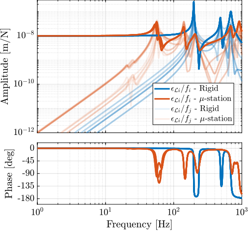

Controller design

<<ssec:nass_hac_controller>>

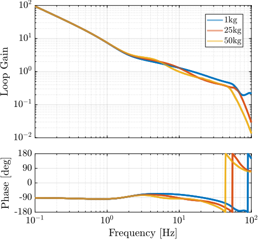
A high authority controller was designed to meet two key requirements: stability for all payload masses (i.e. for all the damped plants of Figure ref:fig:nass_hac_plants), and achievement of sufficient bandwidth (targeted at 10Hz) for high performance operation. The controller structure is defined in Equation eqref:eq:nass_robust_hac, incorporating an integrator term for low frequency performance, a lead compensator for phase margin improvement, and a low-pass filter for robustness against high frequency modes.

\begin{equation}\label{eq:nass_robust_hac} K_{\text{HAC}}(s) = g_0 ⋅ _brace{\frac{ω_c}{s}}_{\text{int}} ⋅ _brace{\frac{1}{\sqrt{α}}\frac{1 + \frac{s}{ω_c/\sqrt{α}}}{1 + \frac{s}{ω_c\sqrt{α}}}}_{\text{lead}} ⋅ _brace{\frac{1}{1 + \frac{s}{ω_0}}}_{\text{LPF}}, \quad ≤ft( ω_c = 2π10\,\text{rad/s},\ α = 2,\ ω_0 = 2π80\,\text{rad/s} \right)

\end{equation}

%% HAC Design
% Wanted crossover
wc = 2*pi*10; % [rad/s]

% Integrator
H_int = wc/s;

% Lead to increase phase margin
a  = 2;  % Amount of phase lead / width of the phase lead / high frequency gain
H_lead = 1/sqrt(a)*(1 + s/(wc/sqrt(a)))/(1 + s/(wc*sqrt(a)));

% Low Pass filter to increase robustness
H_lpf = 1/(1 + s/2/pi/80);

% Gain to have unitary crossover at wc
H_gain = 1./abs(evalfr(G_hac_m50(1,1), 1j*wc));

% Decentralized HAC
Khac = -H_gain  * ... % Gain
        H_int   * ... % Integrator
        H_lead   * ... % Low Pass filter
        H_lpf   * ... % Low Pass filter
        eye(6);       % 6x6 Diagonal

% The designed HAC controller is saved
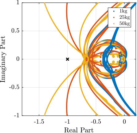
save('./mat/nass_K_hac.mat', 'Khac');

The controller performance was evaluated through two complementary analyses. First, the decentralized loop gain shown in Figure ref:fig:nass_hac_loop_gain, confirms the achievement of the desired 10Hz bandwidth. Second, the characteristic loci analysis presented in Figure ref:fig:nass_hac_loci demonstrates robustness for all payload masses, with adequate stability margins maintained throughout the operating envelope.

Tomography experiment

<<ssec:nass_hac_tomography>>

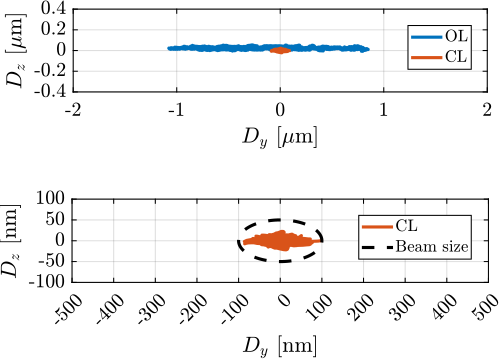
The Nano Active Stabilization System concept was validated through time-domain simulations of scientific experiments, with a particular focus on tomography scanning because of its demanding performance requirements. Simulations were conducted at the maximum operational rotational velocity of $\Omega_z = 360\,\text{deg/s}$ to evaluate system performance under the most challenging conditions.

Performance metrics were established based on anticipated future beamline specifications, which specify a beam size of 200nm (horizontal) by 100nm (vertical). The primary requirement stipulates that the point of interest must remain within beam dimensions throughout operation. The simulation incorporated two principal disturbance sources: ground motion and spindle vibrations. Additional noise sources, including measurement noise and electrical noise from DAC and voltage amplifiers, were not included in this analysis, as these parameters will be optimized during the detailed design phase.

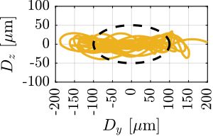
Figure ref:fig:nass_tomo_1kg_60rpm presents a comparative analysis of positioning errors under both open-loop and closed-loop conditions for a lightweight sample configuration (1kg). The results demonstrate the system's capability to maintain the sample's position within the specified beam dimensions, thus validating the fundamental concept of the stabilization system.

%% Simulation of tomography experiments
% Sample is not centered with the rotation axis
% This is done by offsetfing the micro-hexapod by 0.9um
P_micro_hexapod = [0.9e-6; 0; 0]; % [m]

open(mdl);
set_param(mdl, 'StopTime', '2');

initializeGround();
initializeGranite();
initializeTy();
initializeRy();
initializeRz();
initializeMicroHexapod('AP', P_micro_hexapod);
initializeSample('type', 'cylindrical', 'm', 1);

initializeSimscapeConfiguration('gravity', false);
initializeLoggingConfiguration('log', 'all', 'Ts', 1e-3);

initializeDisturbances(...
    'Dw_x',  true, ... % Ground Motion - X direction
    'Dw_y',  true, ... % Ground Motion - Y direction
    'Dw_z',  true, ... % Ground Motion - Z direction
    'Fdy_x', false, ... % Translation Stage - X direction
    'Fdy_z', false, ... % Translation Stage - Z direction
    'Frz_x', true, ... % Spindle - X direction
    'Frz_y', true, ... % Spindle - Y direction
    'Frz_z', true);    % Spindle - Z direction

initializeReferences(...
    'Rz_type', 'rotating', ...
    'Rz_period', 1, ...
    'Dh_pos', [P_micro_hexapod; 0; 0; 0]);

% Open-Loop Simulation without Nano-Hexapod - 1kg payload
initializeSimplifiedNanoHexapod('type', 'none');
initializeController('type', 'open-loop');
sim(mdl);
exp_tomo_ol_m1 = simout;

% Closed-Loop Simulation with NASS
initializeSimplifiedNanoHexapod();
initializeController('type', 'hac-iff');
load('nass_K_iff.mat', 'Kiff');
load('nass_K_hac.mat', 'Khac');

% 1kg payload
initializeSample('type', 'cylindrical', 'm', 1);
sim(mdl);
exp_tomo_cl_m1 = simout;

% 25kg payload
initializeSample('type', 'cylindrical', 'm', 25);
sim(mdl);
exp_tomo_cl_m25 = simout;

% 50kg payload
initializeSample('type', 'cylindrical', 'm', 50);
sim(mdl);
exp_tomo_cl_m50 = simout;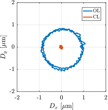

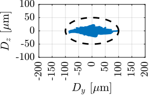
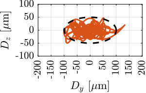
The robustness of the NASS to payload mass variation was evaluated through additional tomography scan simulations with 25 and 50kg payloads, complementing the initial 1kg test case. As illustrated in Figure ref:fig:nass_tomography_hac_iff, system performance exhibits some degradation with increasing payload mass, which is consistent with predictions from the control analysis. While the positioning accuracy for heavier payloads is outside the specified limits, it remains within acceptable bounds for typical operating conditions.

It should be noted that the maximum rotational velocity of 360deg/s is primarily intended for lightweight payload applications. For higher mass configurations, rotational velocities are expected to be below 36deg/s.

Conclusion

<<sec:nass_conclusion>>

The development and analysis presented in this chapter have successfully validated the Nano Active Stabilization System concept, marking the completion of the conceptual design phase. A comprehensive control strategy has been established, effectively combining external metrology with nano-hexapod sensor measurements to achieve precise position control. The control strategy implements a High Authority Control - Low Authority Control architecture - a proven approach that has been specifically adapted to meet the unique requirements of the rotating NASS.

The decentralized Integral Force Feedback component has been demonstrated to provide robust active damping under various operating conditions. The addition of parallel springs to the force sensors has been shown to ensure stability during spindle rotation. The centralized High Authority Controller, operating in the frame of the struts for simplicity, has successfully achieved the desired performance objectives of maintaining a bandwidth of $10\,\text{Hz}$ while maintaining robustness against payload mass variations. This investigation has confirmed that the moderate actuator stiffness of $1\,N/\mu m$ represents an adequate choice for the nano-hexapod, as both very stiff and very compliant configurations introduce significant performance limitations.

Simulations of tomography experiments have been performed, with positioning accuracy requirements defined by the expected minimum beam dimensions of $200\,\text{nm}$ by $100\,\text{nm}$. The system has demonstrated excellent performance at maximum rotational velocity with lightweight samples. While some degradation in positioning accuracy has been observed with heavier payloads, as anticipated by the control analysis, the overall performance remains sufficient to validate the fundamental concept of the NASS.

These results provide a solid foundation for advancing to the subsequent detailed design phase and experimental implementation.

Bibliography   ignore