phd-simscape-nass/simscape-nass.org

Simscape Model - Nano Active Stabilization System

• Introduction
• Control Kinematics
  • Introduction
  • Micro Station Kinematics
  • Computation of the sample's pose error
  • Position error in the frame of the struts
  • Control Architecture - Summary
• Decentralized Active Damping
  • Introduction
  • IFF Plant
  • Controller Design
  • Conclusion
• Centralized Active Vibration Control
  • Introduction
  • HAC Plant
  • Effect of micro-station compliance
  • Higher or lower nano-hexapod stiffness?
  • Controller design
  • Tomography experiment
  • Conclusion
• Conclusion
• Bibliography

Introduction   ignore

From last sections:

• Uniaxial: No stiff nano-hexapod (should also demonstrate that here)
• Rotating: No soft nano-hexapod, Decentralized IFF can be used robustly by adding parallel stiffness
• Micro-Station multi body model tuned from a modal analysis
• Multi-body model of a nano-hexapod that can be merged with the multi-body model of the micro-station

In this section:

• Take the model of the nano-hexapod described in previous section (stiffness 1um/N)
• Control kinematics: how the external metrology, the nano-hexapod metrology are used to control the sample's position (Section ref:sec:nass_kinematics)
• Apply decentralized IFF (Section ref:sec:nass_active_damping)

• Apply HAC-LAC (Section ref:sec:nass_hac)

  • Check robustness to change of payload and to spindle rotation
  • Simulation of experiments
• Conclusion of the conceptual phase, validation with simulations

Control Kinematics

<<sec:nass_kinematics>>

Introduction   ignore

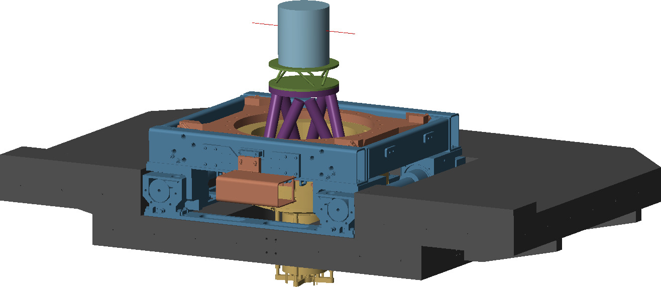
Figure ref:fig:nass_concept_schematic presents a schematic overview of the NASS. This section focuses specifically on the components of the "Instrumentation and Real-Time Control" block.

Schematic of the Nano Active Stabilization System

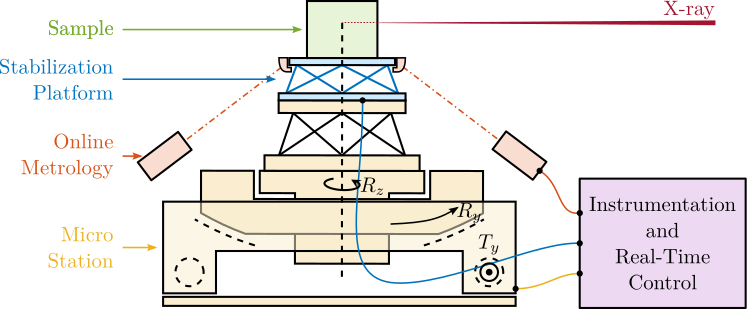
As established in the previous section on Stewart platforms, the proposed control strategy combines Decentralized Integral Force Feedback with a High Authority Controller performed in the frame of the struts.

For the Nano Active Stabilization System, computing the positioning errors in the frame of the struts involves three key steps. First, the system computes the desired sample pose relative to a frame representing the point where the X-ray light is focused using micro-station kinematics, as detailed in Section ref:ssec:nass_ustation_kinematics. Second, it measures the actual sample pose relative to the same fix frame, described in Section ref:ssec:nass_sample_pose_error. Finally, it determines the sample pose error and maps these errors to the nano-hexapod struts, as explained in Section ref:ssec:nass_error_struts.

The complete control architecture is detailed in Section ref:ssec:nass_control_architecture.

Micro Station Kinematics

<<ssec:nass_ustation_kinematics>>

The micro-station kinematics enables the computation of the desired sample pose from the reference signals of each micro-station stage. These reference signals consist of the desired lateral position $r_{D_y}$, tilt angle $r_{R_y}$, and spindle angle $r_{R_z}$. The micro-hexapod pose is defined by six parameters: three translations ($r_{D_{\mu x}}$, $r_{D_{\mu y}}$, $r_{D_{\mu z}}$) and three rotations ($r_{\theta_{\mu x}}$, $r_{\theta_{\mu y}}$, $r_{\theta_{\mu z}}$).

Using these reference signals, the desired sample position relative to the fixed frame is expressed through the homogeneous transformation matrix $\bm{T}_{\mu\text{-station}}$, as defined in equation eqref:eq:nass_sample_ref.

\begin{equation}\label{eq:nass_sample_ref} \bm{T}_{μ\text{-station}} = \bm{T}_{D_y} ⋅ \bm{T}_{R_y} ⋅ \bm{T}_{R_z} ⋅ \bm{T}_{μ\text{-hexapod}}

\end{equation}

\begin{equation}\label{eq:nass_ustation_matrices}

\begin{align} \bm{T}_{D_y} &= \begin{bmatrix} 1 & 0 & 0 & 0 \\ 0 & 1 & 0 & r_{D_y} \\ 0 & 0 & 1 & 0 \\ 0 & 0 & 0 & 1 \end{bmatrix} \quad \bm{T}_{\mu\text{-hexapod}} = \left[ \begin{array}{ccc|c} & & & r_{D_{\mu x}} \\ & \bm{R}_x(r_{\theta_{\mu x}}) \bm{R}_y(r_{\theta_{\mu y}}) \bm{R}_{z}(r_{\theta_{\mu z}}) & & r_{D_{\mu y}} \\ & & & r_{D_{\mu z}} \cr \hline 0 & 0 & 0 & 1 \end{array} \right] \\ \bm{T}_{R_z} &= \begin{bmatrix} \cos(r_{R_z}) & -\sin(r_{R_z}) & 0 & 0 \\ \sin(r_{R_z}) & \cos(r_{R_z}) & 0 & 0 \\ 0 & 0 & 1 & 0 \\ 0 & 0 & 0 & 1 \end{bmatrix} \quad \bm{T}_{R_y} = \begin{bmatrix} \cos(r_{R_y}) & 0 & \sin(r_{R_y}) & 0 \\ 0 & 1 & 0 & 0 \\ -\sin(r_{R_y}) & 0 & \cos(r_{R_y}) & 0 \\ 0 & 0 & 0 & 1 \end{bmatrix} \end{align}

\end{equation}

Computation of the sample's pose error

<<ssec:nass_sample_pose_error>>

The external metrology system measures the sample position relative to the fixed granite. Due to the system's symmetry, this metrology provides measurements for five degrees of freedom: three translations ($D_x$, $D_y$, $D_z$) and two rotations ($R_x$, $R_y$).

The sixth degree of freedom ($R_z$) is still required to compute the errors in the frame of the nano-hexapod struts (i.e. to compute the nano-hexapod inverse kinematics). This $R_z$ rotation is estimated by combining measurements from the spindle encoder and the nano-hexapod's internal metrology, which consists of relative motion sensors in each strut (note that the micro-hexapod is not used for $R_z$ rotation, and is therefore ignore for $R_z$ estimation).

The measured sample pose is represented by the homogeneous transformation matrix $\bm{T}_{\text{sample}}$, as shown in equation eqref:eq:nass_sample_pose.

\begin{equation}\label{eq:nass_sample_pose} \bm{T}_{\text{sample}} = ≤ft[ \begin{array}{ccc|c} & & & D_{x} \\ & \bm{R}_x(R_{x}) \bm{R}_y(R_{y}) \bm{R}_{z}(R_{z}) & & D_{y} \\ & & & D_{z} \cr \hline 0 & 0 & 0 & 1 \end{array} \right]

\end{equation}

Position error in the frame of the struts

<<ssec:nass_error_struts>>

The homogeneous transformation formalism enables straightforward computation of the sample position error. This computation involves the previously computed homogeneous $4 \times 4$ matrices: $\bm{T}_{\mu\text{-station}}$ representing the desired pose, and $\bm{T}_{\text{sample}}$ representing the measured pose. Their combination yields $\bm{T}_{\text{error}}$, which expresses the position error of the sample in the frame of the rotating nano-hexapod, as shown in equation eqref:eq:nass_transformation_error.

\begin{equation}\label{eq:nass_transformation_error} \bm{T}_{\text{error}} = \bm{T}_{μ\text{-station}}^-1 ⋅ \bm{T}_{\text{sample}}

\end{equation}

The known structure of the homogeneous transformation matrix facilitates efficient real-time computation of the inverse. From $\bm{T}_{\text{error}}$, the position and orientation errors $\bm{\epsilon}_{\mathcal{X}} = [\epsilon_{D_x},\ \epsilon_{D_y},\ \epsilon_{D_z},\ \epsilon_{R_x},\ \epsilon_{R_y},\ \epsilon_{R_z}]$ of the sample are extracted using equation eqref:eq:nass_compute_errors:

\begin{equation}\label{eq:nass_compute_errors}

\begin{align} \epsilon_{D_x} & = \bm{T}_{\text{error}}(1,4) \\ \epsilon_{D_y} & = \bm{T}_{\text{error}}(2,4) \\ \epsilon_{D_z} & = \bm{T}_{\text{error}}(3,4) \\ \epsilon_{R_y} & = \text{atan2}(\bm{T}_{\text{error}}(1,3), \sqrt{\bm{T}_{\text{error}}(1,1)^2 + \bm{T}_{\text{error}}(1,2)^2}) \\ \epsilon_{R_x} & = \text{atan2}(-\bm{T}_{\text{error}}(2,3)/\cos(\epsilon_{R_y}), \bm{T}_{\text{error}}(3,3)/\cos(\epsilon_{R_y})) \\ \epsilon_{R_z} & = \text{atan2}(-\bm{T}_{\text{error}}(1,2)/\cos(\epsilon_{R_y}), \bm{T}_{\text{error}}(1,1)/\cos(\epsilon_{R_y})) \\ \end{align}

\end{equation}

Finally, these errors are mapped to the strut space through the nano-hexapod Jacobian matrix eqref:eq:nass_inverse_kinematics.

\begin{equation}\label{eq:nass_inverse_kinematics} \bm{ε}_{\mathcal{L}} = \bm{J} ⋅ \bm{ε}_{\mathcal{X}}

\end{equation}

Control Architecture - Summary

<<ssec:nass_control_architecture>>

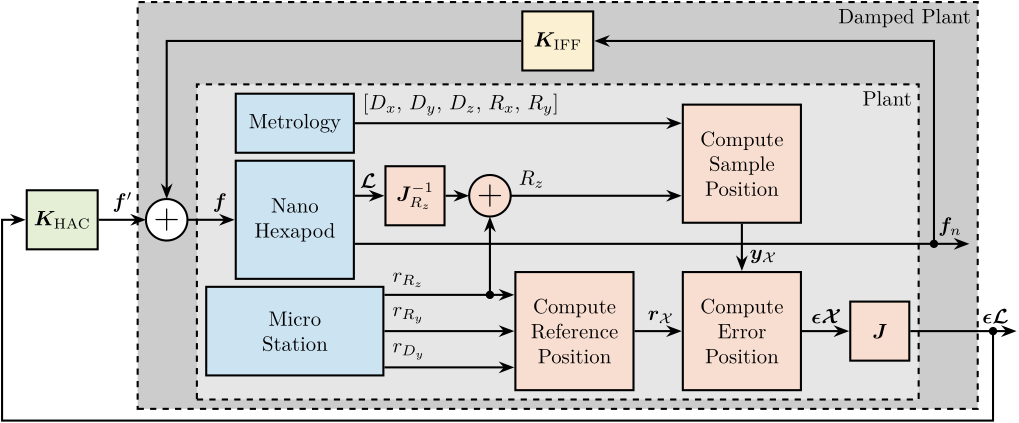
The complete control architecture is summarized in Figure ref:fig:nass_control_architecture. The sample pose is measured using external metrology for five degrees of freedom, while the sixth degree of freedom (Rz) is estimated by combining measurements from the nano-hexapod encoders and spindle encoder.

The sample reference pose is determined by the reference signals of the translation stage, tilt stage, spindle, and micro-hexapod. Position error computation follows a two-step process: first, homogeneous transformation matrices are used to determine the error in the nano-hexapod frame, then the Jacobian matrix $\bm{J}$ maps these errors to individual strut coordinates.

For control purposes, force sensors mounted on each strut are used in a decentralized way for active damping, as detailed in Section ref:sec:nass_active_damping. Then, the high authority controller uses the computed errors in the frame of the struts to provides real-time stabilization of the sample position (Section ref:sec:nass_hac).

\begin{tikzpicture}
  % Blocs
  \node[block={2.0cm}{1.0cm}, fill=colorblue!20!white] (metrology) {Metrology};
  \node[block={2.0cm}{2.0cm}, below=0.1 of metrology, align=center, fill=colorblue!20!white] (nhexa) {Nano\\Hexapod};
  \node[block={3.0cm}{1.5cm}, below=0.1 of nhexa, align=center, fill=colorblue!20!white] (ustation) {Micro\\Station};

  \coordinate[] (inputf)  at ($(nhexa.south west)!0.5!(nhexa.north west)$);
  \coordinate[] (outputfn) at ($(nhexa.south east)!0.3!(nhexa.north east)$);
  \coordinate[] (outputde) at ($(nhexa.south east)!0.7!(nhexa.north east)$);

  \coordinate[] (outputDy) at ($(ustation.south east)!0.1!(ustation.north east)$);
  \coordinate[] (outputRy) at ($(ustation.south east)!0.5!(ustation.north east)$);
  \coordinate[] (outputRz) at ($(ustation.south east)!0.9!(ustation.north east)$);

  \node[block={1.0cm}{1.0cm}, right=0.5 of outputde, fill=colorred!20!white] (Rz_kinematics) {$\bm{J}_{R_z}^{-1}$};
  \node[block={2.0cm}{2.0cm}, right=2.2 of ustation, align=center, fill=colorred!20!white] (ustation_kinematics) {Compute\\Reference\\Position};
  \node[block={2.0cm}{2.0cm}, right=0.8 of ustation_kinematics, align=center, fill=colorred!20!white] (compute_error) {Compute\\Error\\Position};
  \node[block={2.0cm}{2.0cm}, above=0.8 of compute_error, align=center, fill=colorred!20!white] (compute_pos) {Compute\\Sample\\Position};
  \node[block={1.0cm}{1.0cm}, right=0.8 of compute_error, fill=colorred!20!white] (hexa_jacobian) {$\bm{J}$};

  \coordinate[] (inputMetrology) at ($(compute_error.north east)!0.3!(compute_error.north west)$);
  \coordinate[] (inputRz) at ($(compute_error.north east)!0.7!(compute_error.north west)$);

  \node[addb={+}{}{}{}{}, right=0.4 of Rz_kinematics, fill=colorred!20!white] (addRz) {};
  \draw[->] (Rz_kinematics.east) -- (addRz.west);
  \draw[->] (outputRz-|addRz)node[branch]{} -- (addRz.south);

  \draw[->] (outputDy) node[above right]{$r_{D_y}$} -- (outputDy-|ustation_kinematics.west);
  \draw[->] (outputRy) node[above right]{$r_{R_y}$} -- (outputRy-|ustation_kinematics.west);
  \draw[->] (outputRz) node[above right]{$r_{R_z}$} -- (outputRz-|ustation_kinematics.west);

  \draw[->] (metrology.east)node[above right]{$[D_x,\,D_y,\,D_z,\,R_x,\,R_y]$} -- (compute_pos.west|-metrology);
  \draw[->] (addRz.east)node[above right]{$R_z$} -- (compute_pos.west|-addRz);
  \draw[->] (compute_pos.south)node -- (compute_error.north)node[above right]{$\bm{y}_{\mathcal{X}}$};

  \draw[->] (outputde) -- (Rz_kinematics.west) node[above left]{$\bm{\mathcal{L}}$};
  \draw[->] (ustation_kinematics.east) -- (compute_error.west) node[above left]{$\bm{r}_{\mathcal{X}}$};
  \draw[->] (compute_error.east) -- (hexa_jacobian.west) node[above left]{$\bm{\epsilon\mathcal{X}}$};
  \draw[->] (hexa_jacobian.east) -- ++(1.8, 0) node[above left]{$\bm{\epsilon\mathcal{L}}$};

  \draw[->] (outputfn) -- ($(outputfn-|hexa_jacobian.east) + (1.0, 0)$)coordinate(fn) node[above left]{$\bm{f}_n$};

  \begin{scope}[on background layer]
    \node[fit={(metrology.north-|ustation.west) (hexa_jacobian.east|-compute_error.south)}, fill=black!10!white, draw, dashed, inner sep=4pt] (plant) {};
    \node[anchor={north east}] at (plant.north east){$\text{Plant}$};
  \end{scope}

  \node[block, above=0.2 of plant, fill=coloryellow!20!white] (Kiff) {$\bm{K}_{\text{IFF}}$};
  \draw[->] ($(fn)-(0.6,0)$)node[branch]{} |- (Kiff.east);

  \node[addb={+}{}{}{}{}, left=0.8 of inputf] (addf) {};
  \draw[->] (Kiff.west) -| (addf.north);

  \begin{scope}[on background layer]
    \node[fit={(plant.south-|fn) (addf.west|-Kiff.north)}, fill=black!20!white, draw, dashed, inner sep=4pt] (damped_plant) {};
    \node[anchor={north east}] at (damped_plant.north east){$\text{Damped Plant}$};
  \end{scope}

  \begin{scope}[on background layer]
    \node[fit={(metrology.north-|ustation.west) (hexa_jacobian.east|-compute_error.south)}, fill=black!10!white, draw, dashed, inner sep=4pt] (plant) {};
    \node[anchor={north east}] at (plant.north east){$\text{Plant}$};
  \end{scope}

  \node[block, left=0.8 of addf, fill=colorgreen!20!white] (Khac) {$\bm{K}_{\text{HAC}}$};
  \draw[->] ($(hexa_jacobian.east)+(1.4,0)$)node[branch]{} |- ($(Khac.west)+(-0.4, -3.4)$) |- (Khac.west);
  \draw[->] (Khac.east) -- node[midway, above]{$\bm{f}^{\prime}$} (addf.west);
  \draw[->] (addf.east) -- (inputf) node[above left]{$\bm{f}$};
\end{tikzpicture}

Decentralized Active Damping

<<sec:nass_active_damping>>

Introduction   ignore

• How to apply/optimize IFF on an hexapod?
• Robustness to payload mass
• Root Locus
• Damping optimization

Explain which samples are tested:

• cylindrical, 250mm height
• mass of 1kg, 25kg and 50kg

IFF Plant

Using the multi-body model, the transfer functions from the six actuator forces $f_i$ to the six force sensors $f_{mi}$ are computed.

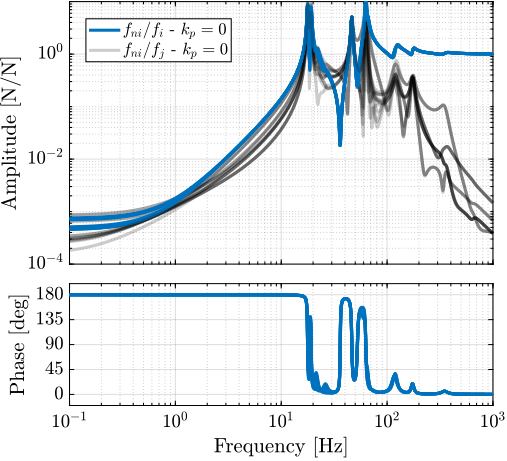
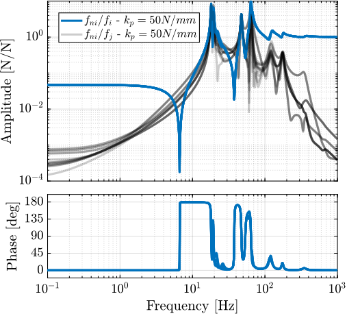
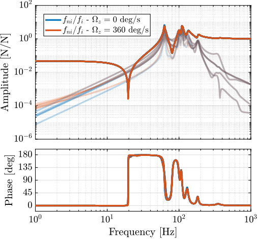
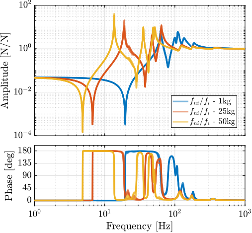
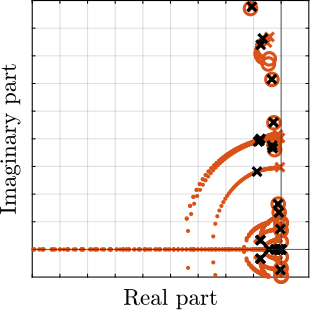
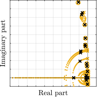
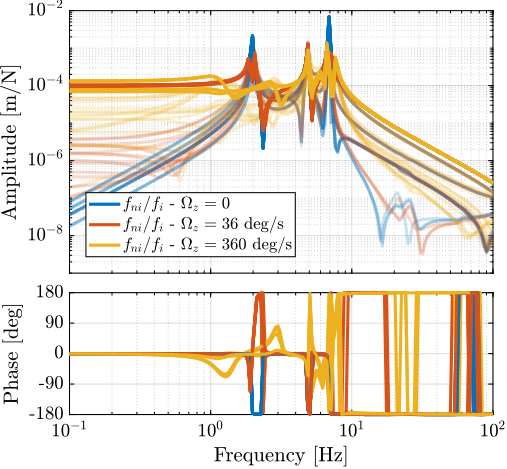
First the effect of added parallel stiffness on the plant dynamics is studied in Figure ref:fig:nass_iff_plant_effect_kp. The plant is identified while the Spindle is rotating at a maximum velocity $\Omega_z = 360\,\text{deg/s}$. The payload mass is 25kg. The obtained dynamics without the parallel stiffness (Figure ref:fig:nass_iff_plant_no_kp) has non-minimum phase zeros at low frequency, as was predicted using the 3-DoF rotating model. When the parallel stiffness is added (Figure ref:fig:nass_iff_plant_kp), a minimum phase complex conjugate zero is obtained instead, which permits to use decentralized IFF with unconditional stability.

In both cases, high coupling around resonances, but should have guaranteed stability thanks to the collocated nature of actuators and sensors.

%% Identify the IFF plant dynamics using the Simscape model

% Initialize each Simscape model elements
initializeGround();
initializeGranite();
initializeTy();
initializeRy();
initializeRz();
initializeMicroHexapod();
initializeSimplifiedNanoHexapod();

% Initial Simscape Configuration
initializeSimscapeConfiguration('gravity', false);
initializeDisturbances('enable', false);
initializeLoggingConfiguration('log', 'none');
initializeController('type', 'open-loop');
initializeReferences();

% Input/Output definition
clear io; io_i = 1;
io(io_i) = linio([mdl, '/Controller'], 1, 'openinput');             io_i = io_i + 1; % Actuator Inputs [N]
io(io_i) = linio([mdl, '/NASS'],       3, 'openoutput', [], 'fn');  io_i = io_i + 1; % Force Sensors [N]

%% Identify for multi payload masses (no rotation)
initializeReferences(); % No Spindle Rotation
% 1kg Sample
initializeSample('type', 'cylindrical', 'm', 1);
G_iff_m1 = linearize(mdl, io);
G_iff_m1.InputName  = {'f1',  'f2',  'f3',  'f4',  'f5',  'f6'};
G_iff_m1.OutputName = {'fn1', 'fn2', 'fn3', 'fn4', 'fn5', 'fn6'};

% 25kg Sample
initializeSample('type', 'cylindrical', 'm', 25);
G_iff_m25 = linearize(mdl, io);
G_iff_m25.InputName  = {'f1',  'f2',  'f3',  'f4',  'f5',  'f6'};
G_iff_m25.OutputName = {'fn1', 'fn2', 'fn3', 'fn4', 'fn5', 'fn6'};

% 50kg Sample
initializeSample('type', 'cylindrical', 'm', 50);
G_iff_m50 = linearize(mdl, io);
G_iff_m50.InputName  = {'f1',  'f2',  'f3',  'f4',  'f5',  'f6'};
G_iff_m50.OutputName = {'fn1', 'fn2', 'fn3', 'fn4', 'fn5', 'fn6'};

%% Effect of Rotation
initializeReferences(...
    'Rz_type', 'rotating', ...
    'Rz_period', 1); % 360 deg/s
initializeSample('type', 'cylindrical', 'm', 25);
G_iff_m25_Rz = linearize(mdl, io, 0.1);
G_iff_m25_Rz.InputName  = {'f1',  'f2',  'f3',  'f4',  'f5',  'f6'};
G_iff_m25_Rz.OutputName = {'fn1', 'fn2', 'fn3', 'fn4', 'fn5', 'fn6'};

%% Effect of Rotation - No added parallel stiffness
initializeSimplifiedNanoHexapod('actuator_kp', 0);
initializeReferences(...
    'Rz_type', 'rotating', ...
    'Rz_period', 1); % 360 deg/s
initializeSample('type', 'cylindrical', 'm', 25);
G_iff_m25_Rz_no_kp = linearize(mdl, io, 0.1);
G_iff_m25_Rz_no_kp.InputName  = {'f1',  'f2',  'f3',  'f4',  'f5',  'f6'};
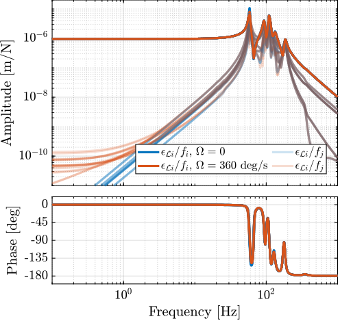
G_iff_m25_Rz_no_kp.OutputName = {'fn1', 'fn2', 'fn3', 'fn4', 'fn5', 'fn6'};

• Effect of Rotation ref:fig:nass_iff_plant_effect_rotation: almost negligible thanks to sufficient actuator stiffness of $1\,\mu m/N$ (determined using the uniaxial model) coupling is increased at much lower frequency that the first mode to damp and should therefore do not impact the control performances
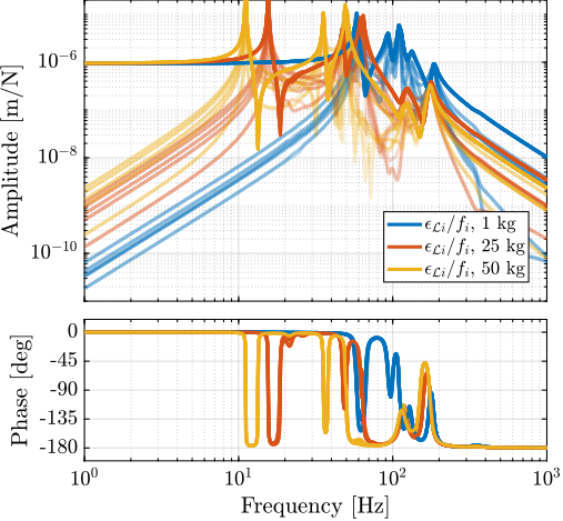
• Effect of payload's mass ref:fig:nass_iff_plant_effect_payload: still have alternating poles and zeros, and therefore bounded phase between 0 and 180 degrees. Location of poles change with the payload's mass as expected.

Controller Design

Using the 3DoF rotating model, it was shown that the decentralized IFF with pure integrators becomes unstable due to gyroscopic induced by the spindle's rotation. It was shown that adding sufficient stiffness in parallel with the force sensor allows to make the decentralized IFF unconditional stable again. Such parallel stiffness are here added to the nano-hexapod, and using the multi-body model of the NASS, it is verified that without parallel stiffness, the system would be unstable when using decentralized IFF with pure integrators.

Even though pure integrators will give stable systems and guaranteed stability when parallel stiffness are added, it would lead to unnecessary gain at low frequency that would modify the damped plant dynamics at low frequency. To avoid that, a second order low pass filter is added at low frequency eqref:eq:nass_kiff.

\begin{equation}\label{eq:nass_kiff} \bm{K}_{\text{IFF}}(s) = g ⋅ \begin{bmatrix} K_{\text{IFF}}(s) & & 0 \\ & \ddots & \\ 0 & & K_{\text{IFF}}(s) \end{bmatrix}, \quad K_{\text{IFF}}(s) = \frac{1}{s} ⋅ \frac{\frac{s^2}{ω_z^2}}{\frac{s^2}{ω_z^2} + 2 ξ_z \frac{s}{ω_z} + 1}

\end{equation}

%% Verify that parallel stiffness permits to have a stable plant
Kiff_pure_int = -200/s*eye(6);
isstable(feedback(G_iff_m1_Rz,       Kiff_pure_int, 1))
isstable(feedback(G_iff_m1_Rz_no_kp, Kiff_pure_int, 1))

%% IFF Controller Design
% Second order high pass filter
wz = 2*pi*2;
xiz = 0.7;
Ghpf = (s^2/wz^2)/(s^2/wz^2 + 2*xiz*s/wz + 1);

Kiff = -200 * ...              % Gain
       1/(0.01*2*pi + s) * ... % LPF: provides integral action
       Ghpf * ...              % 2nd order HPF (limit low frequency gain)
       eye(6);                 % Diagonal 6x6 controller (i.e. decentralized)

Kiff.InputName = {'fm1', 'fm2', 'fm3', 'fm4', 'fm5', 'fm6'};
Kiff.OutputName = {'f1', 'f2', 'f3', 'f4', 'f5', 'f6'};

% The designed IFF controller is saved
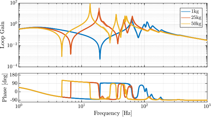
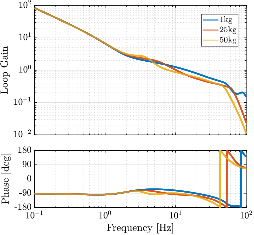
save('./mat/nass_K_iff.mat', 'Kiff');

The frequency of the second order high pass filter is tuned to be below the frequency of the complex conjugate zero for the highest mass (here at $4\,\text{Hz}$). The overall gain is increased to have some authority on the nano-hexapod modes that we want to damp (Figure ref:fig:nass_iff_loop_gain).

Loop gain for the decentralized IFF: $K_{\text{IFF}}(s) \cdot \frac{f_{mi}}{f_i}(s)$

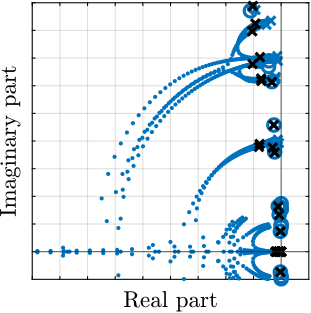
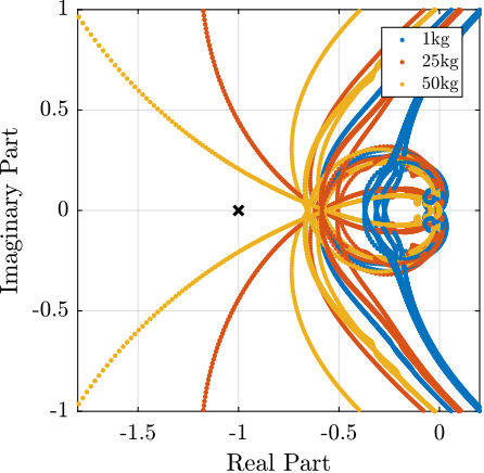
In order to check the stability, root loci for the three payload configurations are computed and shown in Figure ref:fig:nass_iff_root_locus. It is shown that the closed-loop poles are bounded to the left-half plane indicating the good robustness properties of the applied decentralized IFF.

Conclusion

Centralized Active Vibration Control

<<sec:nass_hac>>

Introduction   ignore

• Effect of micro-station compliance Compare plant with "rigid" u-station and normal u-station
• Effect of IFF
• Effect of payload mass
• Decoupled plant
• Controller design

From control kinematics:

• Talk about issue of not estimating Rz from external metrology? (maybe could be nice to discuss that during the experiments!)
• Show what happens is Rz is not estimated (for instance supposed equaled to zero => increased coupling)

HAC Plant

%% Identify the IFF plant dynamics using the Simscape model

% Initialize each Simscape model elements
initializeGround();
initializeGranite();
initializeTy();
initializeRy();
initializeRz();
initializeMicroHexapod();
initializeSimplifiedNanoHexapod();
initializeSample('type', 'cylindrical', 'm', 1);

% Initial Simscape Configuration
initializeSimscapeConfiguration('gravity', false);
initializeDisturbances('enable', false);
initializeLoggingConfiguration('log', 'none');
initializeController('type', 'open-loop');
initializeReferences();

% Input/Output definition
clear io; io_i = 1;
io(io_i) = linio([mdl, '/Controller'],     1, 'input');                  io_i = io_i + 1; % Actuator Inputs [N]
io(io_i) = linio([mdl, '/Tracking Error'], 1, 'openoutput', [], 'EdL');  io_i = io_i + 1; % Strut errors [m]

%% Identify HAC Plant without using IFF
initializeSample('type', 'cylindrical', 'm', 1);
G_m1 = linearize(mdl, io);
G_m1.InputName  = {'f1', 'f2', 'f3', 'f4', 'f5', 'f6'};
G_m1.OutputName = {'l1', 'l2', 'l3', 'l4', 'l5', 'l6'};

initializeSample('type', 'cylindrical', 'm', 25);
G_m25 = linearize(mdl, io);
G_m25.InputName  = {'f1', 'f2', 'f3', 'f4', 'f5', 'f6'};
G_m25.OutputName = {'l1', 'l2', 'l3', 'l4', 'l5', 'l6'};

initializeSample('type', 'cylindrical', 'm', 50);
G_m50 = linearize(mdl, io);
G_m50.InputName  = {'f1', 'f2', 'f3', 'f4', 'f5', 'f6'};
G_m50.OutputName = {'l1', 'l2', 'l3', 'l4', 'l5', 'l6'};

%% Effect of Rotation
initializeSample('type', 'cylindrical', 'm', 1);
initializeReferences(...
    'Rz_type', 'rotating', ...
    'Rz_period', 1); % 360 deg/s

G_m1_Rz = linearize(mdl, io, 0.1);
G_m1_Rz.InputName  = {'f1',  'f2',  'f3',  'f4',  'f5',  'f6'};
G_m1_Rz.OutputName = {'l1', 'l2', 'l3', 'l4', 'l5', 'l6'};

• Effect of rotation: ref:fig:nass_undamped_plant_effect_Wz Add some coupling at low frequency, but still small at the considered velocity. This is thanks to the relatively stiff nano-hexapod (CF rotating model)
• Effect of payload mass: Decrease resonance frequencies Increase coupling: ref:fig:nass_undamped_plant_effect_mass => control challenge for high payload masses
• Other effects such as: Ry tilt angle, Rz spindle position, micro-hexapod position are found to have negligible effect on the plant dynamics. This is thanks to the fact the the plant dynamics is well decoupled from the micro-station dynamics.

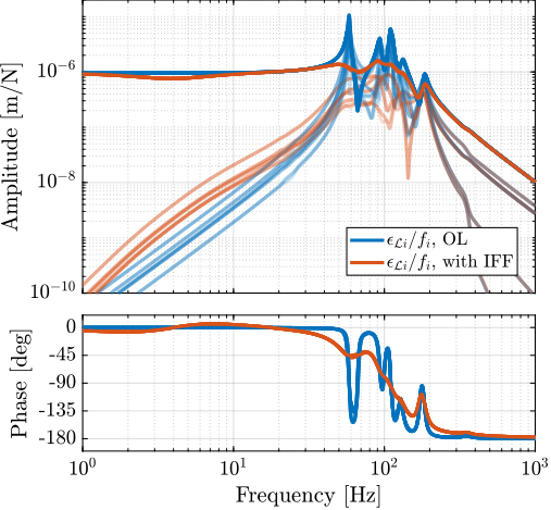
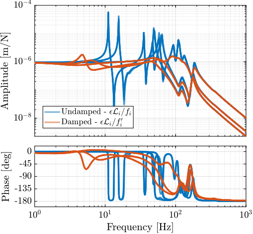
• Effect of IFF on the plant ref:fig:nass_comp_undamped_damped_plant_m1 Modes are well damped Small coupling increase at low frequency
• Benefits of using IFF ref:fig:nass_hac_plants with added damping, the set of plants to be controlled (with payloads from 1kg to 50kg) is more easily controlled. Between 10 and 50Hz, the plant dynamics does not vary a lot with the frequency, whereas without active damping, it would be impossible to design a robust controller with bandwidth above 10Hz that is robust to the change of payload

%% Identify HAC Plant without using IFF
initializeReferences(); % No Spindle Rotation
initializeController('type', 'iff'); % Implemented IFF controller
load('nass_K_iff.mat', 'Kiff'); % Load designed IFF controller

% 1kg payload
initializeSample('type', 'cylindrical', 'm', 1);
G_hac_m1 = linearize(mdl, io);
G_hac_m1.InputName  = {'f1', 'f2', 'f3', 'f4', 'f5', 'f6'};
G_hac_m1.OutputName = {'l1', 'l2', 'l3', 'l4', 'l5', 'l6'};

% 25kg payload
initializeSample('type', 'cylindrical', 'm', 25);
G_hac_m25 = linearize(mdl, io);
G_hac_m25.InputName  = {'f1', 'f2', 'f3', 'f4', 'f5', 'f6'};
G_hac_m25.OutputName = {'l1', 'l2', 'l3', 'l4', 'l5', 'l6'};

% 50kg payload
initializeSample('type', 'cylindrical', 'm', 50);
G_hac_m50 = linearize(mdl, io);
G_hac_m50.InputName  = {'f1', 'f2', 'f3', 'f4', 'f5', 'f6'};
G_hac_m50.OutputName = {'l1', 'l2', 'l3', 'l4', 'l5', 'l6'};

% Check stability
if not(isstable(G_hac_m1) && isstable(G_hac_m25) && isstable(G_hac_m50))
    warning('One of HAC plant is not stable')
end

Effect of micro-station compliance

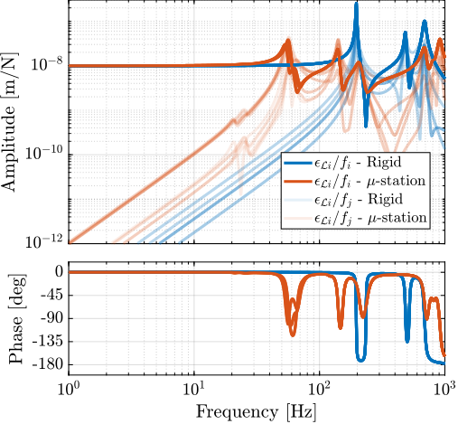
Micro-Station complex dynamics has almost no effect on the plant dynamics (Figure ref:fig:nass_effect_ustation_compliance):

• adds some alternating poles and zeros above 100Hz, which should not be an issue for control

%% Identify plant with "rigid" micro-station
initializeGround('type', 'rigid');
initializeGranite('type', 'rigid');
initializeTy('type', 'rigid');
initializeRy('type', 'rigid');
initializeRz('type', 'rigid');
initializeMicroHexapod('type', 'rigid');
initializeSimplifiedNanoHexapod();
initializeSample('type', 'cylindrical', 'm', 25);

initializeReferences();
initializeController('type', 'open-loop'); % Implemented IFF controller
load('nass_K_iff.mat', 'Kiff'); % Load designed IFF controller

% Input/Output definition
clear io; io_i = 1;
io(io_i) = linio([mdl, '/Controller'],     1, 'input');                  io_i = io_i + 1; % Actuator Inputs [N]
io(io_i) = linio([mdl, '/Tracking Error'], 1, 'openoutput', [], 'EdL');  io_i = io_i + 1; % Strut errors [m]

G_m25_rigid = linearize(mdl, io);
G_m25_rigid.InputName  = {'f1', 'f2', 'f3', 'f4', 'f5', 'f6'};
G_m25_rigid.OutputName = {'l1', 'l2', 'l3', 'l4', 'l5', 'l6'};

Effect of the micro-station limited compliance on the plant dynamics

Higher or lower nano-hexapod stiffness?

Goal: confirm the analysis with simpler models (uniaxial and 3DoF) that a nano-hexapod stiffness of $\approx 1\,N/\mu m$ should give better performances than a very stiff or very soft nano-hexapod.

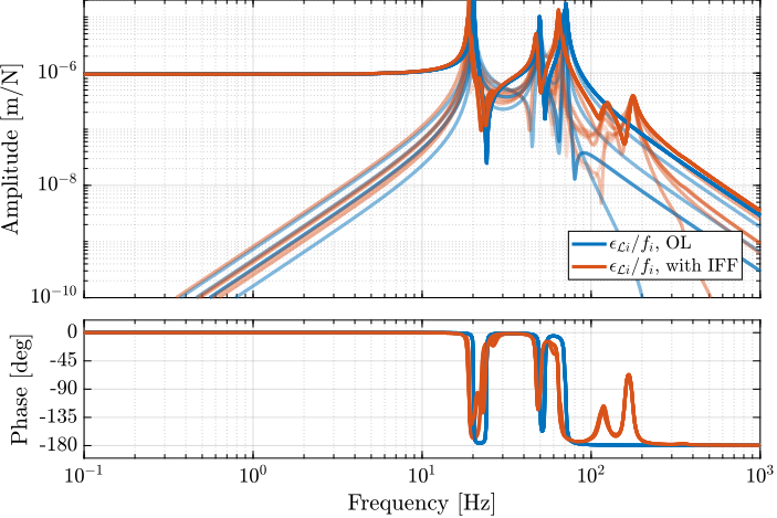
• Stiff nano-hexapod: uniaxial model: high nano-hexapod stiffness induce coupling between the nano-hexapod and the micro-station dynamics. considering the complex dynamics of the micro-station as shown by the modal analysis, that would result in a complex system to control To show that, a nano-hexapod with actuator stiffness equal to 100N/um is initialized, payload of 25kg. The dynamics from $\bm{f}$ to $\bm{\epsilon}_{\mathcal{L}}$ is identified and compared to the case where the micro-station is infinitely rigid (figure ref:fig:nass_stiff_nano_hexapod_coupling_ustation):

  • Coupling induced by the micro-station: much more complex and difficult to model / predict
  • Similar to what was predicted using the uniaxial model

• Soft nano-hexapod: Nano-hexapod with stiffness of 0.01N/um is initialized, payload of 25kg. Dynamics is identified with no spindle rotation, and with spindle rotation of 36deg/s and 360deg/s (Figure ref:fig:nass_soft_nano_hexapod_effect_Wz)

  • Rotation as huge effect on the dynamics: unstable for high rotational velocities, added coupling due to gyroscopic effects, and change of resonance frequencies as a function of the rotational velocity
  • Simple 3DoF rotating model is helpful to understand the complex effect of the rotation => similar conclusion
  • Say that controlling the frame of the struts is not adapted with a soft nano-hexapod, but we should rather control in the frame matching the center of mass of the payload, but we would still obtain large coupling and change of dynamics due to gyroscopic effects.

%% Identify Dynamics with a Stiff nano-hexapod (100N/um)

% Initialize each Simscape model elements
initializeGround();
initializeGranite();
initializeTy();
initializeRy();
initializeRz();
initializeMicroHexapod();
initializeSimplifiedNanoHexapod('actuator_k', 1e8, 'actuator_kp', 0, 'actuator_c', 1e3);
initializeSample('type', 'cylindrical', 'm', 25);

% Initial Simscape Configuration
initializeSimscapeConfiguration('gravity', false);
initializeDisturbances('enable', false);
initializeLoggingConfiguration('log', 'none');
initializeController('type', 'open-loop');
initializeReferences();

% Input/Output definition
clear io; io_i = 1;
io(io_i) = linio([mdl, '/Controller'],     1, 'input');                  io_i = io_i + 1; % Actuator Inputs [N]
io(io_i) = linio([mdl, '/Tracking Error'], 1, 'openoutput', [], 'EdL');  io_i = io_i + 1; % Strut errors [m]

% Identify Plant
G_m25_pz = linearize(mdl, io);
G_m25_pz.InputName  = {'f1', 'f2', 'f3', 'f4', 'f5', 'f6'};
G_m25_pz.OutputName = {'l1', 'l2', 'l3', 'l4', 'l5', 'l6'};

%% Compare with Nano-Hexapod alone (rigid micro-station)
initializeGround('type', 'rigid');
initializeGranite('type', 'rigid');
initializeTy('type', 'rigid');
initializeRy('type', 'rigid');
initializeRz('type', 'rigid');
initializeMicroHexapod('type', 'rigid');

% Identify Plant
G_m25_pz_rigid = linearize(mdl, io);
G_m25_pz_rigid.InputName  = {'f1', 'f2', 'f3', 'f4', 'f5', 'f6'};
G_m25_pz_rigid.OutputName = {'l1', 'l2', 'l3', 'l4', 'l5', 'l6'};

%% Identify Dynamics with a Soft nano-hexapod (0.01N/um)
initializeGround();
initializeGranite();
initializeTy();
initializeRy();
initializeRz();
initializeMicroHexapod();
initializeSimplifiedNanoHexapod('actuator_k', 1e4, 'actuator_kp', 0, 'actuator_c', 1);

% Initialize each Simscape model elements
initializeSample('type', 'cylindrical', 'm', 25); % 25kg payload
initializeController('type', 'open-loop');

% Input/Output definition
clear io; io_i = 1;
io(io_i) = linio([mdl, '/Controller'],     1, 'input');                  io_i = io_i + 1; % Actuator Inputs [N]
io(io_i) = linio([mdl, '/Tracking Error'], 1, 'openoutput', [], 'EdL');  io_i = io_i + 1; % Strut errors [m]

% Identify the dynamics without rotation
initializeReferences();
G_m1_vc = linearize(mdl, io);
G_m1_vc.InputName  = {'f1', 'f2', 'f3', 'f4', 'f5', 'f6'};
G_m1_vc.OutputName = {'l1', 'l2', 'l3', 'l4', 'l5', 'l6'};

% Identify the dynamics with 36 deg/s rotation
initializeReferences(...
    'Rz_type', 'rotating', ...
    'Rz_period', 10); % 36 deg/s

G_m1_vc_Rz_slow = linearize(mdl, io, 0.1);
G_m1_vc_Rz_slow.InputName  = {'f1',  'f2',  'f3',  'f4',  'f5',  'f6'};
G_m1_vc_Rz_slow.OutputName = {'l1', 'l2', 'l3', 'l4', 'l5', 'l6'};

% Identify the dynamics with 360 deg/s rotation
initializeReferences(...
    'Rz_type', 'rotating', ...
    'Rz_period', 1); % 360 deg/s

G_m1_vc_Rz_fast = linearize(mdl, io, 0.1);
G_m1_vc_Rz_fast.InputName  = {'f1',  'f2',  'f3',  'f4',  'f5',  'f6'};
G_m1_vc_Rz_fast.OutputName = {'l1', 'l2', 'l3', 'l4', 'l5', 'l6'};

Controller design

In this section, a high authority controller is design such that:

• it is robust to the change of payload mass (i.e. is should be stable for all the damped plants of Figure ref:fig:nass_hac_plants)
• it has reasonably high bandwidth to give good performances (here 10Hz)

eqref:eq:nass_robust_hac

\begin{equation}\label{eq:nass_robust_hac} K_{\text{HAC}}(s) = g_0 ⋅ _brace{\frac{ω_c}{s}}_{\text{int}} ⋅ _brace{\frac{1}{\sqrt{α}}\frac{1 + \frac{s}{ω_c/\sqrt{α}}}{1 + \frac{s}{ω_c\sqrt{α}}}}_{\text{lead}} ⋅ _brace{\frac{1}{1 + \frac{s}{ω_0}}}_{\text{LPF}}, \quad ≤ft( ω_c = 2π10\,\text{rad/s},\ α = 2,\ ω_0 = 2π80\,\text{rad/s} \right)

\end{equation}

%% HAC Design
% Wanted crossover
wc = 2*pi*10; % [rad/s]

% Integrator
H_int = wc/s;

% Lead to increase phase margin
a  = 2;  % Amount of phase lead / width of the phase lead / high frequency gain
H_lead = 1/sqrt(a)*(1 + s/(wc/sqrt(a)))/(1 + s/(wc*sqrt(a)));

% Low Pass filter to increase robustness
H_lpf = 1/(1 + s/2/pi/80);

% Gain to have unitary crossover at wc
H_gain = 1./abs(evalfr(G_hac_m50(1,1), 1j*wc));

% Decentralized HAC
Khac = -H_gain  * ... % Gain
        H_int   * ... % Integrator
        H_lead   * ... % Low Pass filter
        H_lpf   * ... % Low Pass filter
        eye(6);       % 6x6 Diagonal

% The designed HAC controller is saved
save('./mat/nass_K_hac.mat', 'Khac');

• "Decentralized" Loop Gain: Bandwidth around 10Hz
• Characteristic Loci: Stable for all payloads with acceptable stability margins

Tomography experiment

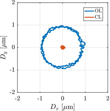
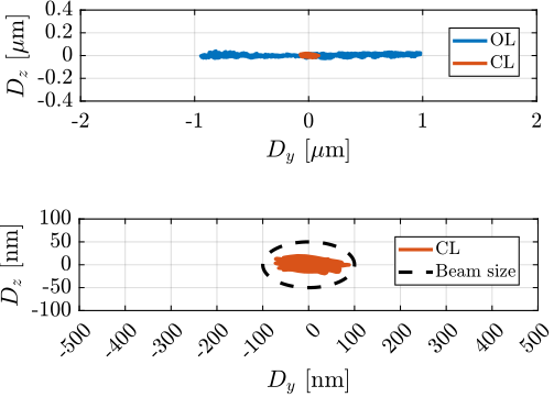
• Validation of concept with tomography scans at the highest rotational velocity of $\Omega_z = 360\,\text{deg/s}$
• Compare obtained results with the smallest beam size that is expected with future beamline upgrade: 200nm (horizontal size) x 100nm (vertical size)
• Take into account the two main sources of disturbances: ground motion, spindle vibrations Other noise sources are not taken into account here as they will be optimized latter (detail design phase): measurement noise, electrical noise for DAC and voltage amplifiers, …

The open-loop errors and the closed-loop errors for the tomography scan with the light sample $1\,kg$ are shown in Figure ref:fig:nass_tomo_1kg_60rpm.

% Sample is not centered with the rotation axis
% This is done by offsetfing the micro-hexapod by 0.9um
P_micro_hexapod = [0.9e-6; 0; 0]; % [m]

open(mdl);
set_param(mdl, 'StopTime', '2');

initializeGround();
initializeGranite();
initializeTy();
initializeRy();
initializeRz();
initializeMicroHexapod('AP', P_micro_hexapod);
initializeSample('type', 'cylindrical', 'm', 1);

initializeSimscapeConfiguration('gravity', false);
initializeLoggingConfiguration('log', 'all', 'Ts', 1e-3);

initializeDisturbances(...
    'Dw_x',  true, ... % Ground Motion - X direction
    'Dw_y',  true, ... % Ground Motion - Y direction
    'Dw_z',  true, ... % Ground Motion - Z direction
    'Fdy_x', false, ... % Translation Stage - X direction
    'Fdy_z', false, ... % Translation Stage - Z direction
    'Frz_x', true, ... % Spindle - X direction
    'Frz_y', true, ... % Spindle - Y direction
    'Frz_z', true);    % Spindle - Z direction

initializeReferences(...
    'Rz_type', 'rotating', ...
    'Rz_period', 1, ...
    'Dh_pos', [P_micro_hexapod; 0; 0; 0]);

% Open-Loop Simulation without Nano-Hexapod - 1kg payload
initializeSimplifiedNanoHexapod('type', 'none');
initializeController('type', 'open-loop');
sim(mdl);
exp_tomo_ol_m1 = simout;

% Closed-Loop Simulation with NASS
initializeSimplifiedNanoHexapod();
initializeController('type', 'hac-iff');
load('nass_K_iff.mat', 'Kiff');
load('nass_K_hac.mat', 'Khac');

% 1kg payload
initializeSample('type', 'cylindrical', 'm', 1);
sim(mdl);
exp_tomo_cl_m1 = simout;

% 25kg payload
initializeSample('type', 'cylindrical', 'm', 25);
sim(mdl);
exp_tomo_cl_m25 = simout;

% 50kg payload
initializeSample('type', 'cylindrical', 'm', 50);
sim(mdl);
exp_tomo_cl_m50 = simout;

% Slower tomography for high payload mass
% initializeReferences(...
%     'Rz_type', 'rotating', ...
%     'Rz_period', 10, ... % 36deg/s
%     'Dh_pos', [P_micro_hexapod; 0; 0; 0]);
% initializeSample('type', 'cylindrical', 'm', 50);
% set_param(mdl, 'StopTime', '5');
% sim(mdl);
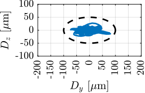
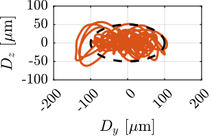
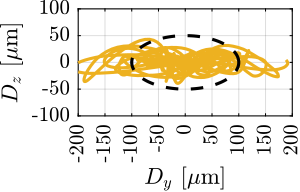
% exp_tomo_cl_m50_slow = simout;

• Effect of payload mass (Figure ref:fig:nass_tomography_hac_iff): Worse performance for high masses, as expected from the control analysis, but still acceptable considering that the rotational velocity of 360deg/s is only used for light payloads.

Conclusion

Conclusion

<<sec:nass_conclusion>>

Bibliography   ignore