phd-simscape-micro-station/simscape-micro-station.org

Simscape Model - Micro Station

• Introduction
• Micro-Station Kinematics
  • Introduction
  • Motion Stages
    • Translation Stage
    • Tilt Stage
    • Spindle
    • Micro-Hexapod
  • Mathematical description of a rigid body motion
    • Introduction
    • Spatial motion representation
    • Motion of a Rigid Body
  • Micro-Station Kinematics
• Micro-Station Dynamics
  • Introduction
  • Multi-Body Model
  • Comparison with the measured dynamics
  • Micro-station compliance
• Estimation of Disturbances
  • Introduction
  • Disturbance measurements
    • Introduction
    • Ground Motion
    • Ty Stage
    • Spindle
  • Sensitivity to disturbances
  • Obtained disturbance sources
• Simulation of Scientific Experiments
  • Introduction
  • Tomography Experiment
  • Raster Scans with the translation stage
• Conclusion
• Bibliography
• Footnotes

Introduction   ignore

Introduction…

Micro-Station Kinematics

<<sec:ustation_kinematics>>

Introduction   ignore

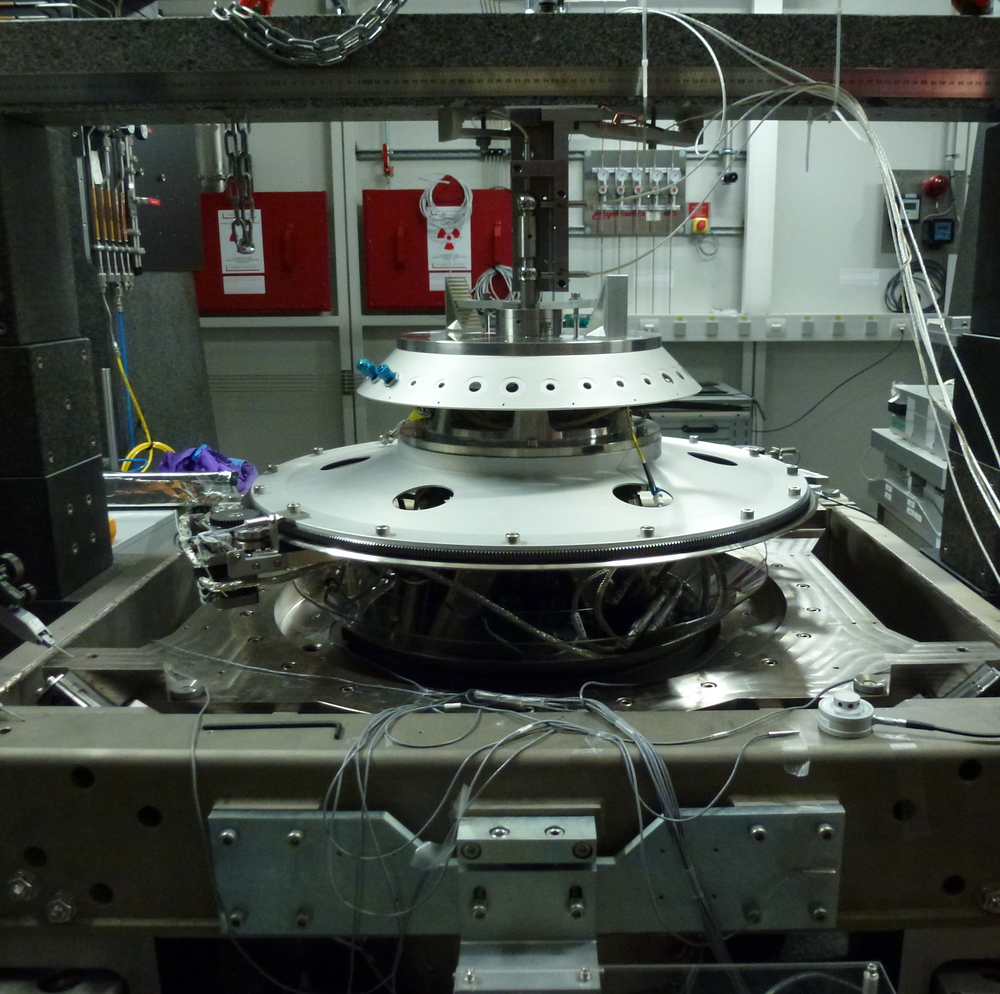
The micro-station consists of 4 stacked positioning stages (Figure ref:fig:ustation_cad_view). From bottom to top, the stacked stages are the translation stage $D_y$, the tilt stage $R_y$, the rotation stage (Spindle) $R_z$ and the positioning hexapod. Such stacked architecture allows high mobility, but the overall stiffness is reduced and the dynamics is very complex. complex dynamics.

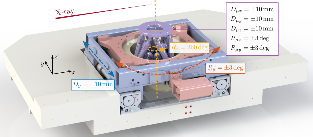
There are different ways of modelling the stage dynamics in a multi-body model. The one chosen in this work consists of modelling each stage by two solid bodies connected by one 6-DoF joint. The stiffness and damping properties of the joint can be tuned separately for each DoF.

The "controlled" DoF of each stage (for instance the $D_y$ direction for the translation stage) is modelled as infinitely rigid (i.e. its motion is imposed by a "setpoint") while the other DoFs have limited stiffness to model the different micro-station modes.

Motion Stages

<<ssec:ustation_stages>>

Translation Stage

The translation stage is used to position and scan the sample laterally with respect to the X-ray beam.

A linear motor was first used to be able to perform fast and accurate scans. It was later replaced with a stepper motor and lead-screw, as the feedback control used for the linear motor was unreliable, probably caused by rust of the linear guides along its stroke. An optical linear encoder is used to measure the stage motion and for PID control of the position.

Four cylindrical bearings¹ are used to guide the motion (i.e. minimize the parasitic motions) and have high stiffness.

Tilt Stage

The tilt stage is guided by four linear motion guides² which are placed such that the center of rotation coincide with the X-ray beam. Each linear guide has high stiffness in radial directions such that the only DoF with low stiffness is in $R_y$.

This stage is mainly used for reflectivity experiments where the sample $R_y$ angle is scanned. This stage can also be used to tilt the rotation axis of the Spindle.

To precisely control the $R_y$ angle, a stepper motor as well as two optical encoders are used in a PID feedback loop.

\hfill

Spindle

Then, a rotation stage is used for tomography experiments. It is composed of an air bearing spindle³, whose angular position is controlled with a 3 phase synchronous motor based on the reading of 4 optical encoders.

Additional rotary unions and slip-rings to be able to pass through the rotation many electrical signals and fluids and gazes.

Micro-Hexapod

Finally, a Stewart platform⁴ is used to position the sample. It includes a DC motor and an optical linear encoders in each of the six strut.

It is used to position the point of interest of the sample with respect to the spindle rotation axis. It can also be used to precisely position the PoI vertically with respect to the x-ray.

\hfill

Mathematical description of a rigid body motion

<<ssec:ustation_motion_description>>

Introduction   ignore

The goal here is to introduce mathematical tools⁵ that are used to describe the motion of positioning stages and ultimately the sample.

First, the tools to described the pose of a solid body (i.e. it's position and orientation) are introduced. Then, the motion induced by a positioning stage is described using transformation matrices. Finally, the motion of all stacked stages are combined, and the sample's motion is computed from each stage motion.

Spatial motion representation

The pose of a solid body with respect to a specific frame can be described by six independent parameters. Three parameters are usually describing its position, and three other parameters are describing its orientation.

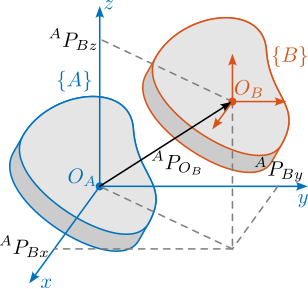
The position of a point $P$ with respect to a frame $\{A\}$ can be described by a $3 \times 1$ position vector eqref:eq:ustation_position. The name of the frame is usually added as a leading superscript: ${}^AP$ which reads as vector $P$ in frame $\{A\}$.

\begin{equation}\label{eq:ustation_position} {}^AP = \begin{bmatrix} P_x\\ P_y\\ P_z \end{bmatrix}

\end{equation}

A pure translation of a solid body (i.e. of a frame $\{B\}$ attached to the solid body) can be described by the position ${}^AP_{O_B}$ as shown in Figure ref:fig:ustation_translation.

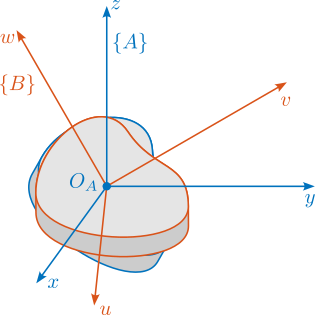
The orientation of a rigid body is the same for all its points (by definition). Hence, the orientation of a rigid body can be viewed as that for the orientation of a moving frame attached to the rigid body. It can be represented in several different ways: the rotation matrix, the screw axis representation and Euler angles are common descriptions.

A rotation matrix ${}^A\mathbf{R}_B$ is a $3 \times 3$ matrix containing the Cartesian unit vectors of frame $\{\mathbf{B}\}$ represented in frame $\{\mathbf{A}\}$ eqref:eq:ustation_rotation_matrix.

\begin{equation}\label{eq:ustation_rotation_matrix} {}^A\mathbf{R}_B = ≤ft[ {}^A\hat{\mathbf{x}}_B | {}^A\hat{\mathbf{y}}_B | {}^A\hat{\mathbf{z}}_B \right] = \begin{bmatrix} u_x & v_x & z_x
u_y & v_y & z_y
u_z & v_z & z_z

\end{bmatrix}

\end{equation}

Consider a pure rotation of a rigid body ($\{\bm{A}\}$ and $\{\bm{B}\}$ are coincident at their origins, as shown in Figure ref:fig:ustation_rotation). The rotation matrix can be used to express the coordinates of a point $P$ in a fixed frame $\{A\}$ (i.e. ${}^AP$) from its coordinate in the moving frame $\{B\}$ using Equation eqref:eq:ustation_rotation.

\begin{equation} \label{eq:ustation_rotation} {}^AP = {}^A\mathbf{R}_B {}^BP

\end{equation}

For rotations along $x$, $y$ or $z$ axis, formulas are given in Equation eqref:eq:ustation_rotation_matrices_xyz.

\begin{subequations}\label{eq:ustation_rotation_matrices_xyz}

\begin{align} \mathbf{R}_x(\theta_x) &= \begin{bmatrix} 1 & 0 & 0 \\ 0 & \cos(\theta_x) & -\sin(\theta_x) \\ 0 & \sin(\theta_x) & \cos(\theta_x) \end{bmatrix} \\ \mathbf{R}_y(\theta_y) &= \begin{bmatrix} \cos(\theta_y) & 0 & \sin(\theta_y) \\ 0 & 1 & 0 \\ -\sin(\theta_y) & 0 & \cos(\theta_y) \end{bmatrix} \\ \mathbf{R}_z(\theta_z) &= \begin{bmatrix} \cos(\theta_z) & -\sin(\theta_z) & 0 \\ \sin(\theta_z) & \cos(\theta_x) & 0 \\ 0 & 0 & 1 \end{bmatrix} \end{align}

\end{subequations}

Sometimes, it is useful to express a rotation as a combination of three rotations described by $\mathbf{R}_x$, $\mathbf{R}_y$ and $\mathbf{R}_z$. As the order of rotation is very important⁶, in this work we choose to express rotations as three successive rotations about the coordinate axes of the moving frame eqref;eq:ustation_rotation_combination.

\begin{equation}\label{eq:ustation_rotation_combination} {}^A\mathbf{R}_B(α, β, γ) = \mathbf{R}_u(α) \mathbf{R}_v(β) \mathbf{R}_c(γ)

\end{equation}

Such rotation can be parameterized by three Euler angles $(\alpha,\ \beta,\ \gamma)$, which can be computed from a given rotation matrix using equations eqref:eq:ustation_euler_angles.

\begin{subequations}\label{eq:ustation_euler_angles}

\begin{align} \alpha &= \text{atan2}(-R_{23}/\cos(\beta),\ R_{33}/\cos(\beta)) \\ \beta &= \text{atan2}( R_{13},\ \sqrt{R_{11}^2 + R_{12}^2}) \\ \gamma &= \text{atan2}(-R_{12}/\cos(\beta),\ R_{11}/\cos(\beta)) \end{align}

\end{subequations}

Motion of a Rigid Body

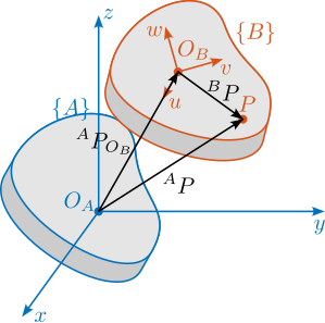
Since the relative positions of a rigid body with respect to a moving frame $\{B\}$ attached to it is fixed for all time, it is sufficient to know the position of the origin of the frame $O_B$ and the orientation of the frame $\{B\}$ with respect to the fixed frame $\{A\}$, to represent the position of any point $P$ in the space.

Therefore, the pose of a rigid body, can be fully determined by:

1. The position vector of point $O_B$ with respect to frame $\{A\}$ which is denoted ${}^AP_{O_B}$
2. The orientation of the rigid body, or the moving frame $\{B\}$ attached to it with respect to the fixed frame $\{A\}$, that is represented by ${}^A\mathbf{R}_B$.

The position of any point $P$ of the rigid body with respect to the fixed frame $\{\mathbf{A}\}$, which is denoted ${}^A\mathbf{P}$ may be determined thanks to the Chasles' theorem, which states that if the pose of a rigid body $\{{}^A\mathbf{R}_B, {}^AP_{O_B}\}$ is given, then the position of any point $P$ of this rigid body with respect to $\{\mathbf{A}\}$ is given by Equation eqref:eq:ustation_chasles_therorem.

\begin{equation} \label{eq:ustation_chasles_therorem} {}^AP = {}^A\mathbf{R}_B {}^BP + {}^AP_{O_B}

\end{equation}

While equation eqref:eq:ustation_chasles_therorem can describe the motion of a rigid body, it can be written in a more convenient way using $4 \times 4$ homogeneous transformation matrices and $4 \times 1$ homogeneous coordinates. The homogeneous transformation matrix is composed of the rotation matrix ${}^A\mathbf{R}_B$ representing the orientation and the position vector ${}^AP_{O_B}$ representing the translation. It is partitioned as shown in Equation eqref:eq:ustation_homogeneous_transformation_parts.

\begin{equation}\label{eq:ustation_homogeneous_transformation_parts} {}^A\mathbf{T}_B = ≤ft[ \begin{array}{ccc|c} & & & \\ & {}^A\mathbf{R}_B & & {}^AP_{O_B} \\ & & & \cr \hline 0 & 0 & 0 & 1 \end{array} \right]

\end{equation}

Then, ${}^AP$ can be computed from ${}^BP$ and the homogeneous transformation matrix using eqref:eq:ustation_homogeneous_transformation.

\begin{equation}\label{eq:ustation_homogeneous_transformation} ≤ft[ \begin{array}{c} \\ {}^AP \\ \cr \hline 1 \end{array} \right] = \left[ \begin{array}{ccc|c} & & & \\ & {}^A\mathbf{R}_B & & {}^AP_{O_B} \\ & & & \cr \hline 0 & 0 & 0 & 1 \end{array} \right] \left[ \begin{array}{c} \\ {}^BP \\ \cr \hline 1 \end{array} \right] = ≤ft[ \begin{array}{ccc|c} & & & \\ & {}^A\mathbf{R}_B & & {}^AP_{O_B} \\ & & & \cr \hline 0 & 0 & 0 & 1 \end{array} \right] \left[ \begin{array}{c} \\ {}^BP \\ \cr \hline 1 \end{array} \right] ≤ft[ \begin{array}{c} \\ {}^BP \\ \cr \hline 1 \end{array} \right] \quad ⇒ \quad {}^AP = {}^A\mathbf{R}_B {}^BP + {}^AP_{O_B}

\end{equation}

One key advantage of using homogeneous transformation is that it can easily be generalized for consecutive transformations. Let us consider the motion of a rigid body described at three locations (Figure ref:fig:ustation_combined_transformation). Frame $\{A\}$ represents the initial location, frame $\{B\}$ is an intermediate location, and frame $\{C\}$ represents the rigid body at its final location.

Motion of a rigid body represented at three locations by frame $\{A\}$, $\{B\}$ and $\{C\}$

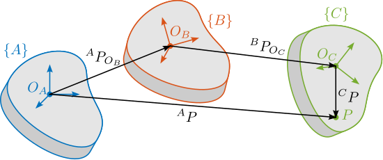
Furthermore, suppose the position vector of a point $P$ of the rigid body is given in the final location, that is ${}^CP$ is given, and the position of this point is to be found in the fixed frame $\{A\}$, that is ${}^AP$. Since the locations of the rigid body is known relative to each other, ${}^CP$ can be transformed to ${}^BP$ using ${}^B\mathbf{T}_C$ using ${}^BP = {}^B\mathbf{T}_C {}^CP$. Similarly, ${}^BP$ can be transformed into ${}^AP$ using ${}^AP = {}^A\mathbf{T}_B {}^BP$.

Combining the two relations, Equation eqref:eq:ustation_consecutive_transformations is obtained. This shows that combining multiple transformations is equivalent as to compute $4 \times 4$ matrix multiplications.

\begin{equation}\label{eq:ustation_consecutive_transformations} {}^AP = _brace{{}^A\mathbf{T}_B {}^B\mathbf{T}_C}_{{}^A\mathbf{T}_C} {}^CP

\end{equation}

Another key advantage of using homogeneous transformation is the easy inverse transformation that can be computed using Equation eqref:eq:ustation_inverse_homogeneous_transformation.

\begin{equation}\label{eq:ustation_inverse_homogeneous_transformation} {}^B\mathbf{T}_A = {}^A\mathbf{T}_B^-1 = ≤ft[ \begin{array}{ccc|c} & & & \\ & {}^A\mathbf{R}_B^T & & -{}^A \mathbf{R}_B^T {}^AP_{O_B} \\ & & & \cr \hline 0 & 0 & 0 & 1 \\ \end{array} \right]

\end{equation}

Micro-Station Kinematics

<<ssec:ustation_kinematics>>

Each stage is described by two frames, one is attached to the fixed platform $\{A\}$ while the other is fixed to the mobile platform $\{B\}$. At "rest" position, the two are having the same pose and coincide with the point of interest ($O_A = O_B$). An example is shown in Figure ref:fig:ustation_stage_motion for the tilt-stage. Note that the mobile frame of the translation stage equals the fixed frame of the tilt stage: $\{B_{D_y}\} = \{A_{R_y}\}$. Similarly, the mobile frame of the tilt stage equals the fixed frame of the spindle: $\{B_{R_y}\} = \{A_{R_z}\}$.

Example of the motion induced by the tilt-stage $R_y$. "Rest" position in shown in blue while a arbitrary position in shown in red. Parasitic motions are here magnified for clarity.

The motion induced by a positioning stage may be described by a homogeneous transformation matrix from frame $\{A\}$ to frame $\{B\}$ as explain in Section ref:ssec:ustation_kinematics. As any motion stage induces parasitic motion in all 6 DoF, the transformation matrix representing its induced motion can be written as in eqref:eq:ustation_translation_stage_errors.

\begin{equation}\label{eq:ustation_translation_stage_errors} {}^A\mathbf{T}_B(D_x, D_y, D_z, θ_x, θ_y, θ_z) = ≤ft[ \begin{array}{ccc|c} & & & D_x \\ & \mathbf{R}_x(\theta_x) \mathbf{R}_y(\theta_y) \mathbf{R}_z(\theta_z) & & D_y \\ & & & D_z \cr \hline 0 & 0 & 0 & 1 \end{array} \right]

\end{equation}

The homogeneous transformation matrix corresponding to the micro-station $\mathbf{T}_{\mu\text{-station}}$ is simply equal to the matrix multiplication of the homogeneous transformation matrices of the individual stages as shown in Equation eqref:eq:ustation_transformation_station.

\begin{equation}\label{eq:ustation_transformation_station} \mathbf{T}_{μ\text{-station}} = \mathbf{T}_{D_y} ⋅ \mathbf{T}_{R_y} ⋅ \mathbf{T}_{R_z} ⋅ \mathbf{T}_{μ\text{-hexapod}}

\end{equation}

$\mathbf{T}_{\mu\text{-station}}$ represents the pose of the sample (supposed to be rigidly fixed on top of the positioning-hexapod) with respect to the granite.

If the transformation matrices of the individual stages are representing a perfect motion (i.e. the stages are supposed to have no parasitic motion), $\mathbf{T}_{\mu\text{-station}}$ is representing the pose setpoint of the sample with respect to the granite. The transformation matrices for the translation stage, tilt stage, spindle and positioning hexapod can be written as shown in Equation eqref:eq:ustation_transformation_matrices_stages.

\begin{equation}\label{eq:ustation_transformation_matrices_stages}

\begin{align} \mathbf{T}_{D_y} &= \begin{bmatrix} 1 & 0 & 0 & 0 \\ 0 & 1 & 0 & D_y \\ 0 & 0 & 1 & 0 \\ 0 & 0 & 0 & 1 \end{bmatrix} \quad \mathbf{T}_{\mu\text{-hexapod}} = \left[ \begin{array}{ccc|c} & & & D_{\mu x} \\ & \mathbf{R}_x(\theta_{\mu x}) \mathbf{R}_y(\theta_{\mu y}) \mathbf{R}_{z}(\theta_{\mu z}) & & D_{\mu y} \\ & & & D_{\mu z} \cr \hline 0 & 0 & 0 & 1 \end{array} \right] \\ \mathbf{T}_{R_z} &= \begin{bmatrix} \cos(\theta_z) & -\sin(\theta_z) & 0 & 0 \\ \sin(\theta_z) & \cos(\theta_z) & 0 & 0 \\ 0 & 0 & 1 & 0 \\ 0 & 0 & 0 & 1 \end{bmatrix} \quad \mathbf{T}_{R_y} = \begin{bmatrix} \cos(\theta_y) & 0 & \sin(\theta_y) & 0 \\ 0 & 1 & 0 & 0 \\ -\sin(\theta_y) & 0 & \cos(\theta_y) & 0 \\ 0 & 0 & 0 & 1 \end{bmatrix} \end{align}

\end{equation}

%% Stage setpoints
Dy = 1e-3; % Translation Stage [m]
Ry = 3*pi/180; % Tilt Stage [rad]
Rz = 180*pi/180; % Spindle [rad]

%% Stage individual Homogeneous transformations
% Translation Stage
Rty = [1 0 0 0;
       0 1 0 Dy;
       0 0 1 0;
       0 0 0 1];

% Tilt Stage - Pure rotating aligned with Ob
Rry = [ cos(Ry) 0 sin(Ry) 0;
        0       1 0       0;
       -sin(Ry) 0 cos(Ry) 0;
        0       0 0       1];

% Spindle - Rotation along the Z axis
Rrz = [cos(Rz) -sin(Rz) 0 0 ;
       sin(Rz)  cos(Rz) 0 0 ;
       0        0       1 0 ;
       0        0       0 1 ];

% Micro-Station homogeneous transformation
Ttot = Rty*Rry*Rrz;

%% Compute translations and rotations (Euler angles) induced by the micro-station
ustation_dx = Ttot(1,4);
ustation_dy = Ttot(2,4);
ustation_dz = Ttot(3,4);
ustation_ry = atan2( Ttot(1, 3),          sqrt(Ttot(1, 1)^2 + Ttot(1, 2)^2));
ustation_rx = atan2(-Ttot(2, 3)/cos(Ery), Ttot(3, 3)/cos(Ery));
ustation_rz = atan2(-Ttot(1, 2)/cos(Ery), Ttot(1, 1)/cos(Ery));

%% Verification using the Simscape model
% All stages are initialized as rigid bodies to avoid any guiding error
initializeGround(      'type', 'rigid');
initializeGranite(     'type', 'rigid');
initializeTy(          'type', 'rigid');
initializeRy(          'type', 'rigid');
initializeRz(          'type', 'rigid');
initializeMicroHexapod('type', 'rigid');

initializeLoggingConfiguration('log', 'all');

initializeReferences('Dy_amplitude', Dy, ...
                     'Ry_amplitude', Ry, ...
                     'Rz_amplitude', Rz);

initializeDisturbances('enable', false);

set_param(conf_simulink, 'StopTime', '0.5');

% Simulation is performed
sim(mdl);

% Sample's motion is computed from "external metrology"
T_sim = [simout.y.R.Data(:,:,end), [simout.y.x.Data(end); simout.y.y.Data(end); simout.y.z.Data(end)]; [0,0,0,1]];
sim_dx = T_sim(1,4);
sim_dy = T_sim(2,4);
sim_dz = T_sim(3,4);
sim_ry = atan2( T_sim(1, 3),          sqrt(T_sim(1, 1)^2 + T_sim(1, 2)^2));
sim_rx = atan2(-T_sim(2, 3)/cos(Ery), T_sim(3, 3)/cos(Ery));
sim_rz = atan2(-T_sim(1, 2)/cos(Ery), T_sim(1, 1)/cos(Ery));

Micro-Station Dynamics

<<sec:ustation_modeling>>

Introduction   ignore

In this section, the Simscape model of the micro-station is briefly presented. It consists of several rigid bodies connected by springs and dampers. The inertia of the solid bodies as well as the stiffness properties of the guiding mechanisms are first estimated based on the CAD model and part data-sheets (Section ref:ssec:ustation_model_simscape).

The obtained dynamics is then compared with the modal analysis performed on the micro-station (Section ref:ssec:ustation_model_comp_dynamics).

As the dynamics of the nano-hexapod is impacted by the micro-station compliance, the most important dynamical characteristic that should be well modeled is the overall compliance of the micro-station. To do so, the 6-DoF compliance of the micro-station is measured and then compared with the 6-DoF compliance extracted from the Simscape model (Section ref:ssec:ustation_model_compliance).

Multi-Body Model

<<ssec:ustation_model_simscape>>

By performing a modal analysis of the micro-station, it could be verified that in the frequency range of interest, each stage behaved as a rigid body. This confirms that a multi-body model can be used to properly model the micro-station.

A multi-body model consists of several solid bodies connected with joints. Each solid body can be represented by inertia properties (most of the time computed automatically from the 3D model and material density). Joints are used to impose kinematic constraints between solid bodies, and to specify dynamical properties (i.e. spring stiffness and damping coefficient). External forces can be used to model disturbances, and "sensors" can be used to measure the relative pose between two defined frames.

Example of a stage (here the tilt-stage) represented in the multi-body model (Simscape). It is composed of two solid bodies connected by a 6-DoF joint. One joint DoF (here the tilt angle) can be imposed, the other ones are represented by springs and dampers. Additional disturbances forces for all DoF can be included

The micro-station is therefore modeled by several solid bodies connected by joints. A typical stage (here the tilt-stage) is modelled as shown in Figure ref:fig:ustation_simscape_stage_example where two solid bodies (the fixed part and the mobile part) are connected by a 6-DoF joint. One DoF of the 6-DoF joint is "imposed" by a setpoint (i.e. modeled as infinitely stiff) while the other 5 are each modelled by a spring and a damper. Additional forces can be used to model disturbances induced by the stage motion. Obtained 3D representation of the multi-body model is shown in Figure ref:fig:ustation_simscape_model.

The Ground is modelled by a solid body connected to the "world frame" through a joint only allowing 3 translations. The granite is then connected to the ground by a 6-DoF joint. The translation stage is connected to the granite by a 6-DoF joint, but the $D_y$ motion is imposed. Similarly, the tilt-stage and the spindle are connected to the stage below using a 6-DoF joint, with 1-DoF being imposed. Finally, the positioning hexapod has 6-DoF.

The total number of "free" degrees of freedom is 27, and therefore the model has 54 states. The springs and dampers values were first estimated from the joints/stages specifications and were later fined tuned based on measurements. The spring values are summarized in Table ref:tab:ustation_6dof_stiffness_values.

Stage	$D_x$	$D_y$	$D_z$	$R_x$	$R_y$	$R_z$
Granite	$5\,kN/\mu m$	$5\,kN/\mu m$	$5\,kN/\mu m$	$25\,Nm/\mu\text{rad}$	$25\,Nm/\mu\text{rad}$	$10\,Nm/\mu\text{rad}$
Translation	$200\,N/\mu m$	-	$200\,N/\mu m$	$60\,Nm/\mu\text{rad}$	$90\,Nm/\mu\text{rad}$	$60\,Nm/\mu\text{rad}$
Tilt	$380\,N/\mu m$	$400\,N/\mu m$	$380\,N/\mu m$	$120\,Nm/\mu\text{rad}$	-	$120\,Nm/\mu\text{rad}$
Spindle	$700\,N/\mu m$	$700\,N/\mu m$	$2\,kN/\mu m$	$10\,Nm/\mu\text{rad}$	$10\,Nm/\mu\text{rad}$	-
Hexapod	$10\,N/\mu m$	$10\,N/\mu m$	$100\,N/\mu m$	$1.5\,Nm/rad$	$1.5\,Nm/rad$	$0.27\,Nm/rad$

Comparison with the measured dynamics

<<ssec:ustation_model_comp_dynamics>>

The dynamics of the micro-station was measured by placing accelerometers on each stage and by impacting the translation stage with an instrumented hammer in three directions. The obtained FRF were then projected at the CoM of each stage.

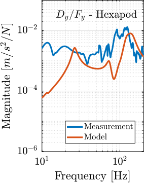
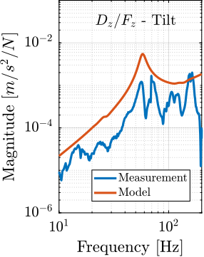
In order to have a first idea of the accuracy of the obtained model, the FRF from the hammer impacts to the acceleration of each stage is extracted from the Simscape model and compared with the measurements in Figure ref:fig:ustation_comp_com_response.

Even though there is some similarity between the model and the measurements (similar overall shapes and amplitudes), it is clear that the Simscape model does not represent very accurately the complex micro-station dynamics. Tuning the numerous model parameters to better match the measurements is an highly non-linear optimization problem which is difficult to solve in practice.

%% Indentify the model dynamics from the 3 hammer imapcts
% To the motion of each solid body at their CoM

% All stages are initialized
initializeGround(      'type', 'rigid');
initializeGranite(     'type', 'flexible');
initializeTy(          'type', 'flexible');
initializeRy(          'type', 'flexible');
initializeRz(          'type', 'flexible');
initializeMicroHexapod('type', 'flexible');

initializeLoggingConfiguration('log', 'none');

initializeReferences();
initializeDisturbances('enable', false);

% Input/Output definition
clear io; io_i = 1;
io(io_i) = linio([mdl, '/Micro-Station/Translation Stage/Flexible/F_hammer'],          1, 'openinput');  io_i = io_i + 1;
io(io_i) = linio([mdl, '/Micro-Station/Granite/Flexible/accelerometer'],               1, 'openoutput'); io_i = io_i + 1;
io(io_i) = linio([mdl, '/Micro-Station/Translation Stage/Flexible/accelerometer'],     1, 'openoutput'); io_i = io_i + 1;
io(io_i) = linio([mdl, '/Micro-Station/Tilt Stage/Flexible/accelerometer'],            1, 'openoutput'); io_i = io_i + 1;
io(io_i) = linio([mdl, '/Micro-Station/Spindle/Flexible/accelerometer'],               1, 'openoutput'); io_i = io_i + 1;
io(io_i) = linio([mdl, '/Micro-Station/Micro Hexapod/Flexible/accelerometer'],         1, 'openoutput'); io_i = io_i + 1;

% Run the linearization
G_ms = linearize(mdl, io, 0);
G_ms.InputName  = {'Fx', 'Fy', 'Fz'};
G_ms.OutputName = {'gtop_x', 'gtop_y', 'gtop_z', 'gtop_rx', 'gtop_ry', 'gtop_rz', ...
                   'ty_x', 'ty_y', 'ty_z', 'ty_rx', 'ty_ry', 'ty_rz', ...
                   'ry_x', 'ry_y', 'ry_z', 'ry_rx', 'ry_ry', 'ry_rz', ...
                   'rz_x', 'rz_y', 'rz_z', 'rz_rx', 'rz_ry', 'rz_rz', ...
                   'hexa_x', 'hexa_y', 'hexa_z', 'hexa_rx', 'hexa_ry', 'hexa_rz'};

% Load estimated FRF at CoM
load('ustation_frf_matrix.mat', 'freqs');
load('ustation_frf_com.mat', 'frfs_CoM');

% Initialization of some variables to the figures
dirs = {'x', 'y', 'z', 'rx', 'ry', 'rz'};
stages = {'gbot', 'gtop', 'ty', 'ry', 'rz', 'hexa'}
f = logspace(log10(10), log10(500), 1000);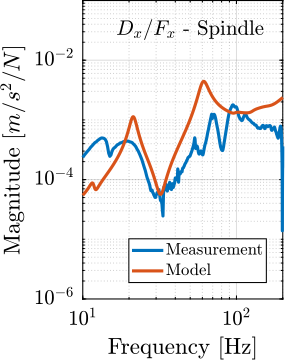

Micro-station compliance

<<ssec:ustation_model_compliance>>

As was shown in the previous section, the dynamics of the micro-station is complex and tuning the multi-body model parameters to obtain a perfect match is hard.

When considering the NASS, the most important dynamical characteristics of the micro-station is its compliance as it is what can impact the plant dynamics. The adopted strategy is therefore to accurately model the micro-station compliance.

The micro-station compliance is experimentally measured using the setup schematically shown in Figure ref:fig:ustation_compliance_meas. Four 3-axis accelerometers are fixed to the micro-hexapod top platform. The micro-hexapod top platform is impacted at 10 different points. For each impact position, 10 impacts are performed for averaging and improving the data quality.

Schematic of the measurement setup to estimate the compliance of the micro-station. The top platform of the positioning hexapod is shown with four 3-axis accelerometers (shown in red) are on top. 10 hammer impacts are performed at different locations (shown in blue).

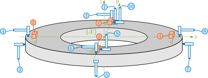
To convert the 12 acceleration signals $a_{\mathcal{L}} = [a_{1x}\ a_{1y}\ a_{1z}\ a_{2x}\ \dots\ a_{4z}]$ to the acceleration expressed in the frame $\{\mathcal{X}\}$ $a_{\mathcal{X}} = [a_{dx}\ a_{dy}\ a_{dz}\ a_{rx}\ a_{ry}\ a_{rz}]$, a Jacobian matrix $\mathbf{J}_a$ is written based on the positions and orientations of the accelerometers eqref:eq:ustation_compliance_acc_jacobian.

\begin{equation}\label{eq:ustation_compliance_acc_jacobian} \mathbf{J}_a = \begin{bmatrix} 1 & 0 & 0 & 0 & 0 &-d
0 & 1 & 0 & 0 & 0 & 0
0 & 0 & 1 & d & 0 & 0
1 & 0 & 0 & 0 & 0 & 0
0 & 1 & 0 & 0 & 0 &-d
0 & 0 & 1 & 0 & d & 0
1 & 0 & 0 & 0 & 0 & d
0 & 1 & 0 & 0 & 0 & 0
0 & 0 & 1 &-d & 0 & 0
1 & 0 & 0 & 0 & 0 & 0
0 & 1 & 0 & 0 & 0 & d
0 & 0 & 1 & 0 &-d & 0

\end{bmatrix}

\end{equation}

Then, the acceleration in the cartesian frame can be computed using eqref:eq:ustation_compute_cart_acc.

\begin{equation}\label{eq:ustation_compute_cart_acc} a_{\mathcal{X}} = \mathbf{J}_a^† ⋅ a_{\mathcal{L}}

\end{equation}

Similar to what is done for the accelerometers, a Jacobian matrix $\mathbf{J}_F$ is computed eqref:eq:ustation_compliance_force_jacobian and used to convert the individual hammer forces $F_{\mathcal{L}}$ to force and torques $F_{\mathcal{X}}$ applied at the center of the micro-hexapod top plate (defined by frame $\{\mathcal{X}\}$ in Figure ref:fig:ustation_compliance_meas).

\begin{equation}\label{eq:ustation_compliance_force_jacobian} \mathbf{J}_F = \begin{bmatrix} 0 & -1 & 0 & 0 & 0 & 0
0 & 0 & -1 & -d & 0 & 0
1 & 0 & 0 & 0 & 0 & 0
0 & 0 & -1 & 0 & -d & 0
0 & 1 & 0 & 0 & 0 & 0
0 & 0 & -1 & d & 0 & 0
-1 & 0 & 0 & 0 & 0 & 0
0 & 0 & -1 & 0 & d & 0
-1 & 0 & 0 & 0 & 0 & -d
-1 & 0 & 0 & 0 & 0 & d

\end{bmatrix}

\end{equation}

Force and torques applied at center of $\{\mathcal{X}\}$ are then computed using eqref:eq:ustation_compute_cart_force.

\begin{equation}\label{eq:ustation_compute_cart_force} F_{\mathcal{X}} = \mathbf{J}_F^t ⋅ F_{\mathcal{L}}

\end{equation}

Using the two Jacobian matrices, the FRF from the 10 hammer impacts to the 12 accelerometer outputs can be converted to the FRF from 6 forces/torques applied at the origin of frame $\{\mathcal{X}\}$ to the 6 linear/angular accelerations of the top platform expressed with respect to $\{\mathcal{X}\}$. These FRF will be used for comparison with the Simscape model.

% Positions and orientation of accelerometers
% | *Num* | *Position* | *Orientation* | *Sensibility* | *Channels* |
% |-------+------------+---------------+---------------+------------|
% |     1 | [0, +A, 0] | [x, y, z]     | 1V/g          |        1-3 |
% |     2 | [-B, 0, 0] | [x, y, z]     | 1V/g          |        4-6 |
% |     3 | [0, -A, 0] | [x, y, z]     | 0.1V/g        |        7-9 |
% |     4 | [+B, 0, 0] | [x, y, z]     | 1V/g          |      10-12 |
%

% Measuerment channels
%
% | Acc Number | Dir | Channel Number |
% |------------+-----+----------------|
% |          1 | x   |              1 |
% |          1 | y   |              2 |
% |          1 | z   |              3 |
% |          2 | x   |              4 |
% |          2 | y   |              5 |
% |          2 | z   |              6 |
% |          3 | x   |              7 |
% |          3 | y   |              8 |
% |          3 | z   |              9 |
% |          4 | x   |             10 |
% |          4 | y   |             11 |
% |          4 | z   |             12 |
% |     Hammer |     |             13 |

% 10 measurements corresponding to 10 different Hammer impact locations
% | *Num* | *Direction* | *Position* | Accelerometer position | Jacobian number |
% |-------+-------------+------------+------------------------+-----------------|
% |     1 | -Y          | [0, +A, 0] |                      1 |              -2 |
% |     2 | -Z          | [0, +A, 0] |                      1 |              -3 |
% |     3 | X           | [-B, 0, 0] |                      2 |               4 |
% |     4 | -Z          | [-B, 0, 0] |                      2 |              -6 |
% |     5 | Y           | [0, -A, 0] |                      3 |               8 |
% |     6 | -Z          | [0, -A, 0] |                      3 |              -9 |
% |     7 | -X          | [+B, 0, 0] |                      4 |             -10 |
% |     8 | -Z          | [+B, 0, 0] |                      4 |             -12 |
% |     9 | -X          | [0, -A, 0] |                      3 |              -7 |
% |    10 | -X          | [0, +A, 0] |                      1 |              -1 |


%% Jacobian for accelerometers
% aX = Ja . aL
d = 0.14; % [m]
Ja = [1  0  0  0  0 -d;
      0  1  0  0  0  0;
      0  0  1  d  0  0;
      1  0  0  0  0  0;
      0  1  0  0  0 -d;
      0  0  1  0  d  0;
      1  0  0  0  0  d;
      0  1  0  0  0  0;
      0  0  1 -d  0  0;
      1  0  0  0  0  0;
      0  1  0  0  0  d;
      0  0  1  0 -d  0];

Ja_inv = pinv(Ja);

%% Jacobian for hammer impacts
% F = Jf' tau
Jf = [0 -1  0  0  0  0;
      0  0 -1 -d  0  0;
      1  0  0  0  0  0;
      0  0 -1  0 -d  0;
      0  1  0  0  0  0;
      0  0 -1  d  0  0;
     -1  0  0  0  0  0;
      0  0 -1  0  d  0;
     -1  0  0  0  0 -d;
     -1  0  0  0  0  d]';
Jf_inv = pinv(Jf);

%% Load raw measurement data
% "Track1" to "Track12" are the 12 accelerometers
% "Track13" is the instrumented hammer force sensor
data = [
    load('ustation_compliance_hammer_1.mat'), ...
    load('ustation_compliance_hammer_2.mat'), ...
    load('ustation_compliance_hammer_3.mat'), ...
    load('ustation_compliance_hammer_4.mat'), ...
    load('ustation_compliance_hammer_5.mat'), ...
    load('ustation_compliance_hammer_6.mat'), ...
    load('ustation_compliance_hammer_7.mat'), ...
    load('ustation_compliance_hammer_8.mat'), ...
    load('ustation_compliance_hammer_9.mat'), ...
    load('ustation_compliance_hammer_10.mat')];

%% Prepare the FRF computation
Ts = 1e-3; % Sampling Time [s]
Nfft = floor(1/Ts); % Number of points for the FFT computation
win = ones(Nfft, 1); % Rectangular window
[~, f] = tfestimate(data(1).Track13, data(1).Track1, win, [], Nfft, 1/Ts);

% Samples taken before and after the hammer "impact"
pre_n = floor(0.1/Ts);
post_n = Nfft - pre_n - 1;

%% Compute the FRFs for the 10 hammer impact locations.
% The FRF from hammer force the 12 accelerometers are computed
% for each of the 10 hammer impacts and averaged
G_raw = zeros(12,10,length(f));

for i = 1:10 % For each impact location
    % Find the 10 impacts
    [~, impacts_i] = find(diff(data(i).Track13 > 50)==1);
    % Only keep the first 10 impacts if there are more than 10 impacts
    if length(impacts_i)>10
        impacts_i(11:end) = [];
    end

    % Average the FRF for the 10 impacts
    for impact_i = impacts_i
        i_start = impact_i - pre_n;
        i_end = impact_i + post_n;
        data_in = data(i).Track13(i_start:i_end); % [N]
        % Remove hammer DC offset
        data_in  = data_in  - mean(data_in(end-pre_n:end));
        % Combine all outputs [m/s^2]
        data_out = [data(i).Track1( i_start:i_end); ...
                    data(i).Track2( i_start:i_end); ...
                    data(i).Track3( i_start:i_end); ...
                    data(i).Track4( i_start:i_end); ...
                    data(i).Track5( i_start:i_end); ...
                    data(i).Track6( i_start:i_end); ...
                    data(i).Track7( i_start:i_end); ...
                    data(i).Track8( i_start:i_end); ...
                    data(i).Track9( i_start:i_end); ...
                    data(i).Track10(i_start:i_end); ...
                    data(i).Track11(i_start:i_end); ...
                    data(i).Track12(i_start:i_end)];

        [frf, ~] = tfestimate(data_in, data_out', win, [], Nfft, 1/Ts);
        G_raw(:,i,:) = squeeze(G_raw(:,i,:)) + 0.1*frf'./(-(2*pi*f').^2);
    end
end

%% Compute transfer function in cartesian frame using Jacobian matrices
% FRF_cartesian = inv(Ja) * FRF * inv(Jf)
FRF_cartesian = pagemtimes(Ja_inv, pagemtimes(G_raw, Jf_inv));

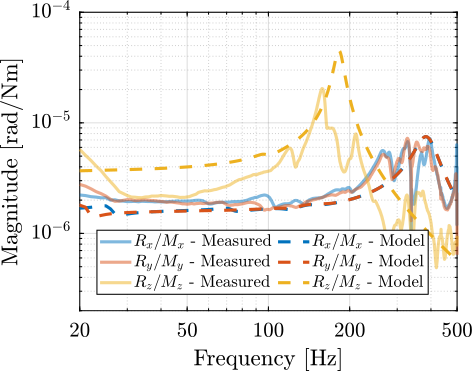
The compliance of the micro-station multi-body model is extracted by computing the transfer function from forces/torques applied to the positioning hexapod's top platform to the "absolute" motion of the top platform. These are compared with the measurements in Figure ref:fig:ustation_frf_compliance_model. Considering how complex the micro-station compliance dynamics is, the model compliance is matching sufficiently well the measurements for the current application.

%% Identification of the compliance of the micro-station

% Initialize simulation with default parameters (flexible elements)
initializeGround();
initializeGranite();
initializeTy();
initializeRy();
initializeRz();
initializeMicroHexapod();

initializeReferences();
initializeSimscapeConfiguration();
initializeLoggingConfiguration();

% Input/Output definition
clear io; io_i = 1;
io(io_i) = linio([mdl, '/Micro-Station/Micro Hexapod/Flexible/Fm'], 1, 'openinput');       io_i = io_i + 1; % Direct Forces/Torques applied on the micro-hexapod top platform
io(io_i) = linio([mdl, '/Micro-Station/Micro Hexapod/Flexible/Dm'], 1, 'output'); io_i = io_i + 1; % Absolute displacement of the top platform

% Run the linearization
Gm = linearize(mdl, io, 0);
Gm.InputName  = {'Fmx', 'Fmy', 'Fmz', 'Mmx', 'Mmy', 'Mmz'};
Gm.OutputName = {'Dx', 'Dy', 'Dz', 'Drx', 'Dry', 'Drz'};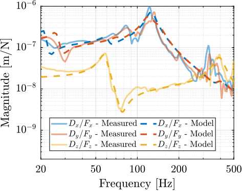

Estimation of Disturbances

<<sec:ustation_disturbances>>

Introduction   ignore

The goal in this section is to obtain realistic representation of disturbances affecting the micro-station. These disturbance sources will then be used during time domain simulations to accurately model the micro-station behavior. The focus is made on stochastic disturbances, as it is in principle possible to calibrate the repeatable part of disturbances. Such disturbance includes ground motion, and vibrations induces by the scanning of the translation stage and the spindle.

In the multi-body model, stage vibrations are modelled as internal forces applied in the stage's joint. In practice, the disturbance forces cannot be directly measured, and the effect of those perturbations on the vibration of the micro-station's top platform is measured instead (Section ref:ssec:ustation_disturbances_meas).

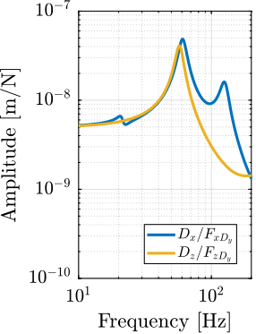
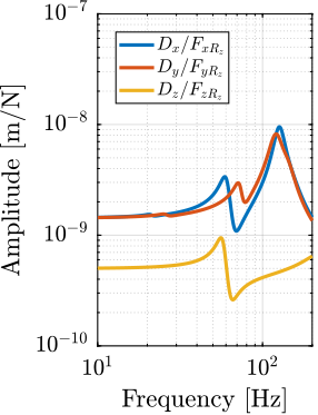
To estimate the equivalent disturbance force that induces such vibration, the transfer function from disturbances sources (i.e. forces applied in the stages' joint) to the displacement of the micro-station's top platform with respect to the granite are extracted from the Simscape model (Section ref:ssec:ustation_disturbances_sensitivity). Finally, the obtained disturbance sources are compared in Section ref:ssec:ustation_disturbances_results.

Disturbance measurements

<<ssec:ustation_disturbances_meas>>

Introduction   ignore

In this section, the ground motion disturbances is directly measured using geophones. Vibrations induced by the scanning of the translation stage and of the spindle are also measured using dedicated setups.

The tilt stage and the micro-hexapod also have positioning errors, they are however not modelled here as these two stages are only used for pre-positioning and not for scanning. Therefore, from a control point of view, they are not important.

Ground Motion

The ground motion is simply measured by using a sensitive 3-axis geophone placed on the ground. The generated voltages are recorded with a high resolution DAC, and converted to displacement using the Geophone sensitivity transfer function. The obtained ground motion displacement is shown in Figure ref:fig:ustation_ground_disturbance.

%% Compute Floor Motion Spectral Density
% Load floor motion data
% t: time in [s]
% V: measured voltage genrated by the geophone and amplified by a 60dB gain voltage amplifier [V]
load('ustation_ground_motion.mat', 't', 'V');

% Geophone Transfer Function
Tg = 88; % Sensitivity [V/(m/s)]
w0 = 2*2*pi; % Cut-off frequency [rad/s]
xi = 0.7; % Damping ratio

G_geo = Tg*s*s^2/(s^2 + 2*xi*w0*s + w0^2); % Geophone's transfer function [V/m]

% Voltage amplifier transfer function
g0 = 10^(60/20); % [abs]

% Compute measured voltage PSD
Ts = (t(2)-t(1)); % Sampling Time [s]
Nfft = floor(2/Ts);
win = hanning(Nfft);
Noverlap = floor(Nfft/2);

[pxx_V, f_gm] = pwelch(V, win, Noverlap, Nfft, 1/Ts); % [V^2/Hz]

% Ground Motion ASD
pxx_gm_z = pxx_V./abs(squeeze(freqresp(G_geo*g0, f_gm, 'Hz'))).^2; % [m^2/Hz]
% Assumption here that horizontal ground motion is ~25% smaller
% than vertical one.
pxx_gm_x = (0.7)^2*pxx_gm_z; % [m^2/Hz]
pxx_gm_y = (0.8)^2*pxx_gm_z; % [m^2/Hz]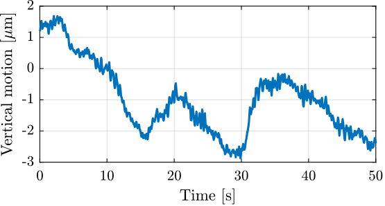

Measured ground motion

Ty Stage

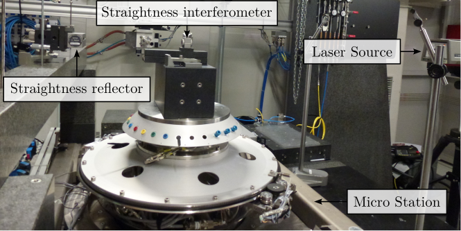
To measure the positioning errors of the translation stage, the setup shown in Figure ref:fig:ustation_errors_ty_setup is used. A special optical element (called a "straightness interferometer"⁷) is fixed on top of the micro-station, while a laser source⁸ and a straightness reflector are fixed on the ground. A similar setup is used to measure the horizontal deviation (i.e. in the $x$ direction), as well as the pitch and yaw errors of the translation stage.

Experimental setup to measure the flatness (vertical deviation) of the translation stage

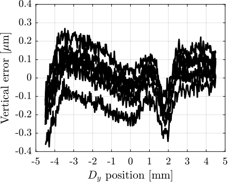
Six scans are performed between $-4.5\,mm$ and $4.5\,mm$. The results for each individual scan are shown in Figure ref:fig:ustation_errors_dy_vertical. As the measurement axis may not be perfectly aligned with the displacement axis of the translation stage, a linear fit may be removed from the measurement. The remaining vertical displacement is shown in Figure ref:fig:ustation_errors_dy_vertical_remove_mean. A vertical error of $\pm300\,nm$ induced by the translation stage is to be expected. Similar result is obtain for the $x$ lateral direction.

%% Ty errors
% Setpoint is in [mm]
% Vertical error is in [um]
ty_errors = load('ustation_errors_ty.mat');

% Compute best straight line to remove it from data
average_error = mean(ty_errors.ty_z')';
straight_line = average_error - detrend(average_error, 1);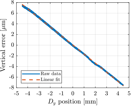

%% Convert the data to frequency domain
% Suppose a certain constant velocity scan
delta_ty = (ty_errors.setpoint(end) - ty_errors.setpoint(1))/(length(ty_errors.setpoint) - 1); % [mm]
ty_vel = 8*1.125; % [mm/s]
Ts = delta_ty/ty_vel;
Fs = 1/Ts

% Frequency Analysis
Nfft = floor(length(ty_errors.setpoint)); % Number of frequency points
win = hanning(Nfft); % Windowing
Noverlap = floor(Nfft/2); % Overlap for frequency analysis

% Comnpute the power spectral density
[pxx_dy_dz, f_dy] = pwelch(1e-6*detrend(ty_errors.ty_z, 1), win, Noverlap, Nfft, Fs);
pxx_dy_dz = mean(pxx_dy_dz')';

% Having the PSD of the lateral error equal to the PSD of the vertical error
% is a reasonable assumption (and verified in practice)
pxx_dy_dx = pxx_dy_dz;

Spindle

In order to measure the positioning errors induced by the Spindle, a "Spindle error analyzer"⁹ is used as shown in Figure ref:fig:ustation_rz_meas_lion_setup. A specific target is fixed on top of the micro-station which consists of two sphere with 1 inch diameter precisely aligned with the spindle rotation axis. Five capacitive sensors¹⁰ are pointing at the two spheres as shown in Figure ref:fig:ustation_rz_meas_lion_zoom. From the 5 measured displacements $[d_1,\,d_2,\,d_3,\,d_4,\,d_5]$, the translations and rotations $[D_x,\,D_y,\,D_z,\,R_x,\,R_y]$ of the target can be estimated.

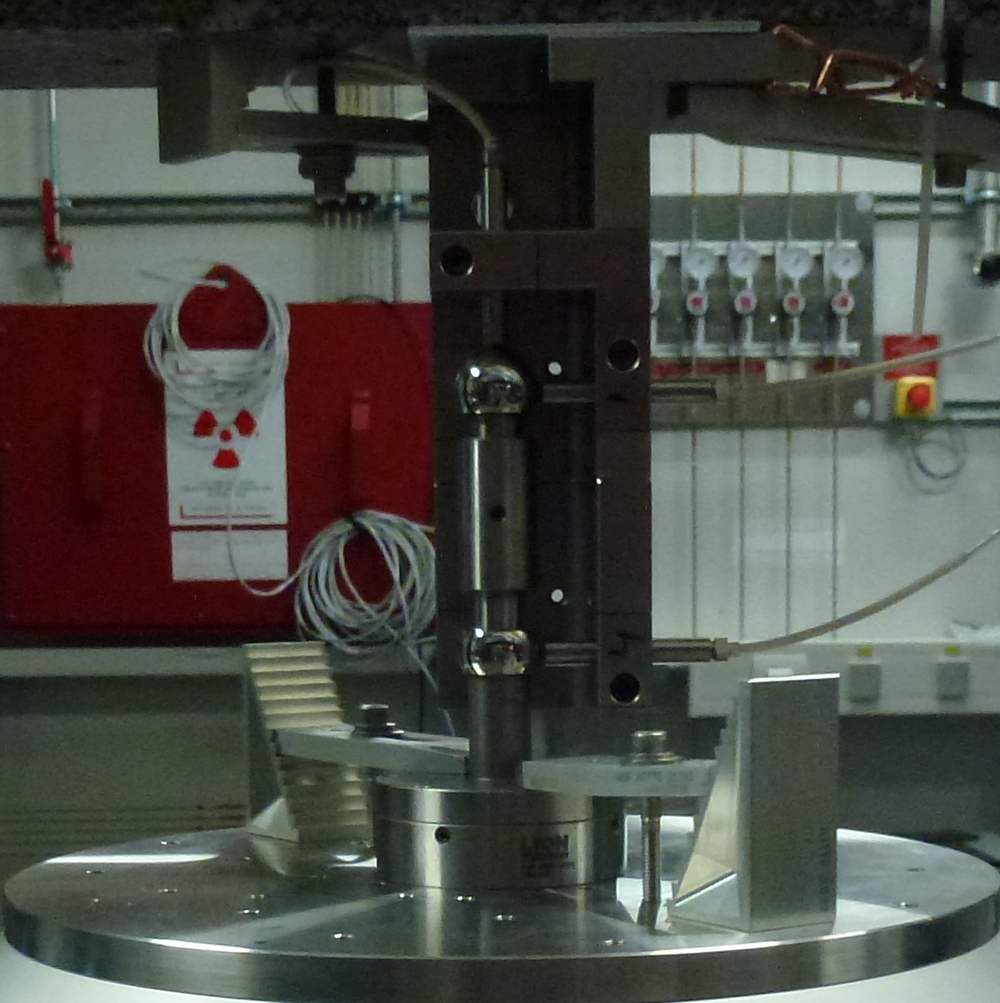
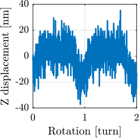
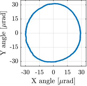
A measurement is performed at 60rpm during 10 turns, and the obtained results are shown in Figure ref:fig:ustation_errors_spindle. A fraction of the radial (Figure ref:fig:ustation_errors_spindle_radial) and tilt (Figure ref:fig:ustation_errors_spindle_tilt) errors is linked to the fact that the two spheres are not perfectly aligned with the rotation axis of the Spindle. This is displayed by the dashed circle. After removing the best circular fit from the data, the vibrations induced by the Spindle may be viewed as stochastic disturbances. However, some misalignment between the "point-of-interest" of the sample with the rotation axis will be considered as it is very difficult to align in practice. The NASS will be used to actively keep the PoI on the rotation axis. The vertical motion induced by the scanning of the spindle is in the order of $\pm 30\,nm$ (Figure ref:fig:ustation_errors_spindle_axial).

%% Spindle Errors
% Errors are already converted to x,y,z,Rx,Ry
% Units are in [m] and [rad]
spindle_errors = load('ustation_errors_spindle.mat');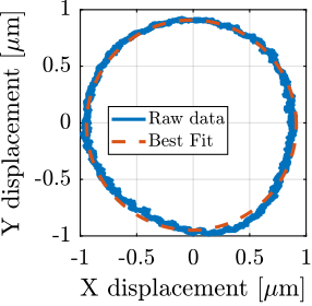

%% Remove the circular fit from the data
[x0, y0, R] = circlefit(spindle_errors.Dx, spindle_errors.Dy);

% Search the best angular match
fun = @(theta)rms((spindle_errors.Dx - (x0 + R*cos(pi/180*spindle_errors.deg+theta(1)))).^2 + (spindle_errors.Dy - (y0 - R*sin(pi/180*spindle_errors.deg+theta(1)))).^2);
x0 = [0];
delta_theta = fminsearch(fun, 0)

% Compute the remaining error after removing the best circular fit
spindle_errors.Dx_err = spindle_errors.Dx - (x0 + R*cos(pi/180*spindle_errors.deg+delta_theta));
spindle_errors.Dy_err = spindle_errors.Dy - (y0 - R*sin(pi/180*spindle_errors.deg+delta_theta));

%% Convert the data to frequency domain
Ts = (spindle_errors.t(end) - spindle_errors.t(1))/(length(spindle_errors.t)-1); % [s]
Fs = 1/Ts; % [Hz]

% Frequency Analysis
Nfft = floor(2.0*Fs); % Number of frequency points
win = hanning(Nfft); % Windowing
Noverlap = floor(Nfft/2); % Overlap for frequency analysis

% Comnpute the power spectral density
[pxx_rz_dz, f_rz] = pwelch(spindle_errors.Dz,     win, Noverlap, Nfft, Fs);
[pxx_rz_dx, ~   ] = pwelch(spindle_errors.Dx_err, win, Noverlap, Nfft, Fs);
[pxx_rz_dy, ~   ] = pwelch(spindle_errors.Dy_err, win, Noverlap, Nfft, Fs);

Sensitivity to disturbances

<<ssec:ustation_disturbances_sensitivity>>

In order to compute the disturbance source (i.e. forces) that induced the measured vibrations in Section ref:ssec:ustation_disturbances_meas, the transfer function from the disturbance sources to the stage vibration (i.e. the "sensitivity to disturbances") needs to be estimated. This is done using the multi-body that was presented in Section ref:sec:ustation_modeling. The obtained transfer functions are shown in Figure ref:fig:ustation_model_sensitivity.

%% Extract sensitivity to disturbances from the Simscape model
% Initialize stages
initializeGround();
initializeGranite();
initializeTy();
initializeRy();
initializeRz();
initializeMicroHexapod();

initializeDisturbances('enable', false);
initializeSimscapeConfiguration('gravity', false);
initializeLoggingConfiguration();

% Configure inputs and outputs
clear io; io_i = 1;
io(io_i) = linio([mdl, '/Disturbances/Dwx'], 1, 'openinput'); io_i = io_i + 1; % Vertical Ground Motion
io(io_i) = linio([mdl, '/Disturbances/Dwy'], 1, 'openinput'); io_i = io_i + 1; % Vertical Ground Motion
io(io_i) = linio([mdl, '/Disturbances/Dwz'], 1, 'openinput'); io_i = io_i + 1; % Vertical Ground Motion
io(io_i) = linio([mdl, '/Disturbances/Fdy_x'], 1, 'openinput'); io_i = io_i + 1; % Parasitic force Ty
io(io_i) = linio([mdl, '/Disturbances/Fdy_z'], 1, 'openinput'); io_i = io_i + 1; % Parasitic force Ty
io(io_i) = linio([mdl, '/Disturbances/Frz_x'], 1, 'openinput'); io_i = io_i + 1; % Parasitic force Rz
io(io_i) = linio([mdl, '/Disturbances/Frz_y'], 1, 'openinput'); io_i = io_i + 1; % Parasitic force Rz
io(io_i) = linio([mdl, '/Disturbances/Frz_z'], 1, 'openinput'); io_i = io_i + 1; % Parasitic force Rz
io(io_i) = linio([mdl, '/Micro-Station/metrology_6dof/x'], 1, 'openoutput'); io_i = io_i + 1; % Relative motion - Hexapod/Granite
io(io_i) = linio([mdl, '/Micro-Station/metrology_6dof/y'], 1, 'openoutput'); io_i = io_i + 1; % Relative motion - Hexapod/Granite
io(io_i) = linio([mdl, '/Micro-Station/metrology_6dof/z'], 1, 'openoutput'); io_i = io_i + 1; % Relative motion - Hexapod/Granite

% Run the linearization
Gd = linearize(mdl, io, 0);
Gd.InputName  = {'Dwx', 'Dwy', 'Dwz', 'Fdy_x', 'Fdy_z', 'Frz_x', 'Frz_y', 'Frz_z'};
Gd.OutputName = {'Dx', 'Dy', 'Dz'};

% The identified dynamics are then saved for further use.
save('./mat/ustation_disturbance_sensitivity.mat', 'Gd')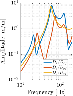

Obtained disturbance sources

<<ssec:ustation_disturbances_results>>

From the measured effect of disturbances in Section ref:ssec:ustation_disturbances_meas and the sensitivity to disturbances extracted from the Simscape model in Section ref:ssec:ustation_disturbances_sensitivity, the power spectral density of the disturbance sources (i.e. forces applied in the stage's joint) can be estimated. They are shown in Figure ref:fig:ustation_dist_sources.

%% Compute the PSD of the equivalent disturbance sources
pxx_rz_fx = pxx_rz_dx./abs(squeeze(freqresp(Gd('Dx', 'Frz_x'), f_rz, 'Hz'))).^2;
pxx_rz_fy = pxx_rz_dy./abs(squeeze(freqresp(Gd('Dy', 'Frz_y'), f_rz, 'Hz'))).^2;
pxx_rz_fz = pxx_rz_dz./abs(squeeze(freqresp(Gd('Dz', 'Frz_z'), f_rz, 'Hz'))).^2;

pxx_dy_fx = pxx_dy_dx./abs(squeeze(freqresp(Gd('Dx', 'Fdy_x'), f_dy, 'Hz'))).^2;
pxx_dy_fz = pxx_dy_dz./abs(squeeze(freqresp(Gd('Dz', 'Fdy_z'), f_dy, 'Hz'))).^2;

%% Save the PSD of the disturbance sources for further used
% in the Simscape model

% Ground motion
min_f = 1; max_f = 500;
gm_dist.f  = f_gm(f_gm < max_f & f_gm > min_f);
gm_dist.pxx_x = pxx_gm_x(f_gm < max_f & f_gm > min_f);
gm_dist.pxx_y = pxx_gm_y(f_gm < max_f & f_gm > min_f);
gm_dist.pxx_z = pxx_gm_z(f_gm < max_f & f_gm > min_f);

% Translation stage
min_f = 0.5; max_f = 500;
dy_dist.f  = f_dy(f_dy < max_f & f_dy > min_f);
dy_dist.pxx_fx = pxx_dy_fx(f_dy < max_f & f_dy > min_f);
dy_dist.pxx_fz = pxx_dy_fz(f_dy < max_f & f_dy > min_f);

% Spindle
min_f = 1; max_f = 500;
rz_dist.f  = f_rz(f_rz < max_f & f_rz > min_f);
rz_dist.pxx_fx = pxx_rz_fx(f_rz < max_f & f_rz > min_f);
rz_dist.pxx_fy = pxx_rz_fy(f_rz < max_f & f_rz > min_f);
rz_dist.pxx_fz = pxx_rz_fz(f_rz < max_f & f_rz > min_f);

% The identified dynamics are then saved for further use.
save('./mat/ustation_disturbance_psd.mat', 'rz_dist', 'dy_dist', 'gm_dist')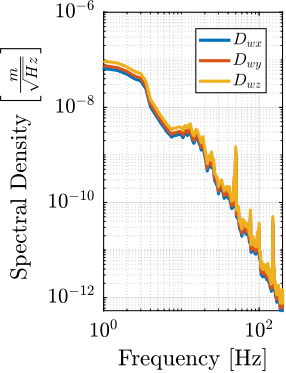

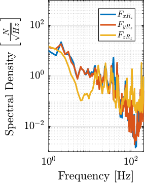
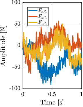
The disturbances are characterized by their power spectral densities as shown in Figure ref:fig:ustation_dist_sources. However, in order to perform time domain simulations, disturbances needs to be represented by a time domain. In order to generate stochastic time domain signals having the same power spectral densities as the ones estimated, the discrete inverse Fourier transform is used as explained in cite:&preumont94_random_vibrat_spect_analy chap. 12.11. Examples of obtained time domain disturbance signals are shown in Figure ref:fig:ustation_dist_sources_time.

%% Compute time domain disturbance signals
initializeDisturbances();
load('nass_model_disturbances.mat');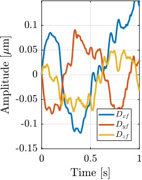

Simulation of Scientific Experiments

<<sec:ustation_experiments>>

Introduction   ignore

In order to fully validate the micro-station multi-body model, two time domain simulations corresponding to typical use cases are performed.

First, a tomography experiment (i.e. a constant Spindle rotation) is performed and compared with experimental measurements (Section ref:sec:ustation_experiments_tomography). Second, a constant velocity scans with the translation stage is performed and also compared with experimental data (Section ref:sec:ustation_experiments_ty_scans).

Tomography Experiment

<<sec:ustation_experiments_tomography>>

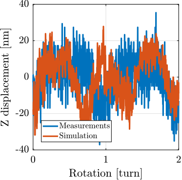
To simulate a tomography experiment, the setpoint of the Spindle is configured to perform a constant rotation with a rotational velocity of 60rpm. Both ground motion and spindle vibration disturbances are simulation based on what was computed in Section ref:sec:ustation_disturbances. A radial offset of $\approx 1\,\mu m$ between the "point-of-interest" and the spindle's rotation axis is introduced to represent what is experimentally observed. During the 10 second simulation (i.e. 10 spindle turns), the position of the "point-of-interest" with respect to the granite is recorded. Results are shown in Figure ref:fig:ustation_errors_model_spindle. A good correlation with the measurements are observed both for radial errors (Figure ref:fig:ustation_errors_model_spindle_radial) and axial errors (Figure ref:fig:ustation_errors_model_spindle_axial).

%% Tomography experiment
% Sample is not centered with the rotation axis
% This is done by offsetfing the micro-hexapod by 0.9um
P_micro_hexapod = [0.9e-6; 0; 0]; % [m]

set_param(conf_simulink, 'StopTime', '10');

initializeGround();
initializeGranite();
initializeTy();
initializeRy();
initializeRz();
initializeMicroHexapod('AP', P_micro_hexapod);

initializeSimscapeConfiguration('gravity', false);
initializeLoggingConfiguration('log', 'all');

initializeDisturbances(...
    'Dw_x',  true, ... % Ground Motion - X direction
    'Dw_y',  true, ... % Ground Motion - Y direction
    'Dw_z',  true, ... % Ground Motion - Z direction
    'Fdy_x', false, ... % Translation Stage - X direction
    'Fdy_z', false, ... % Translation Stage - Z direction
    'Frz_x', true, ... % Spindle - X direction
    'Frz_y', true, ... % Spindle - Y direction
    'Frz_z', true);    % Spindle - Z direction

initializeReferences(...
    'Rz_type', 'rotating', ...
    'Rz_period', 1, ...
    'Dh_pos', [P_micro_hexapod; 0; 0; 0]);

sim(mdl);
exp_tomography = simout;

%% Compare with the measurements
spindle_errors = load('ustation_errors_spindle.mat');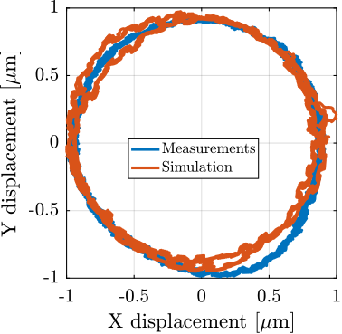

Raster Scans with the translation stage

<<sec:ustation_experiments_ty_scans>>

A second experiment is performed in which the translation stage is scanned with a constant velocity. The translation stage setpoint is configured to have a "triangular" shape with stroke of $\pm 4.5\, mm$. Both ground motion and translation stage vibrations are included in the simulation. Similar to what was performed for the tomography simulation, the PoI position with respect to the granite is recorded and compared with experimental measurements in Figure ref:fig:ustation_errors_model_dy_vertical. Similar error amplitude can be observed, thus indicating that the multi-body model with included disturbances is accurately representing the micro-station behavior for typical scientific experiments.

%% Translation stage latteral scans
set_param(conf_simulink, 'StopTime', '2');

initializeGround();
initializeGranite();
initializeTy();
initializeRy();
initializeRz();
initializeMicroHexapod();

initializeSimscapeConfiguration('gravity', false);
initializeLoggingConfiguration('log', 'all');

initializeDisturbances(...
    'Dw_x',  true, ... % Ground Motion - X direction
    'Dw_y',  true, ... % Ground Motion - Y direction
    'Dw_z',  true, ... % Ground Motion - Z direction
    'Fdy_x', true, ... % Translation Stage - X direction
    'Fdy_z', true, ... % Translation Stage - Z direction
    'Frz_x', false, ... % Spindle - X direction
    'Frz_y', false, ... % Spindle - Y direction
    'Frz_z', false);    % Spindle - Z direction

initializeReferences(...
    'Dy_type', 'triangular', ...
    'Dy_amplitude', 4.5e-3, ...
    'Dy_period', 2);

sim(mdl);
exp_latteral_scans = simout;

% Load the experimentally measured errors
ty_errors = load('ustation_errors_ty.mat');

% Compute best straight line to remove it from data
average_error = mean(ty_errors.ty_z')';
straight_line = average_error - detrend(average_error, 1);

% Only plot data for the scan from -4.5mm to 4.5mm
dy_setpoint = 1e3*exp_latteral_scans.y.y.Data(exp_latteral_scans.y.y.time > 0.5 & exp_latteral_scans.y.y.time < 1.5);
dz_error = detrend(1e6*exp_latteral_scans.y.z.Data(exp_latteral_scans.y.y.time > 0.5 & exp_latteral_scans.y.y.time < 1.5), 0);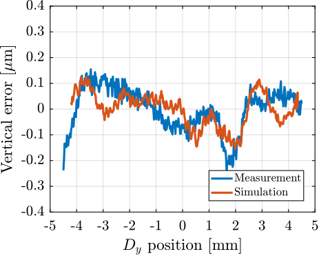

Vertical errors during a constant velocity scan of the translation stage. Comparison of the measurements and simulated errors.

Conclusion

<<sec:uniaxial_conclusion>>

In order to have good model:

• kinematics
• dynamics
• disturbances

Validated with time domain simulations.

Bibliography   ignore

Footnotes

⁸Laser source is manufactured by Agilent (5519b) ⁷The special optics (straightness interferometer and reflector) are manufactured by Agilent (10774A). ¹⁰C8 capacitive sensors and CPL290 capacitive driver electronics from Lion Precision ⁹The Spindle Error Analyzer is made by Lion Precision. ⁵The tools presented here are largely taken from cite:&taghirad13_paral. ⁶Rotations are non commutative in 3D ¹Ball cage (N501) and guide bush (N550) from Mahr are used ⁴Modified Zonda Hexapod by Symetrie ³Made by LAB Motion Systems ²HCR 35 A C1, from THK

---