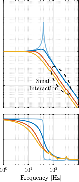
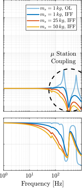
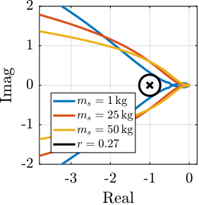
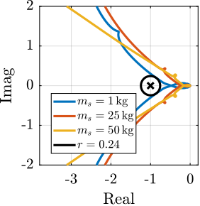
298 KiB
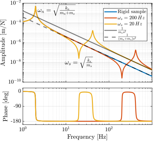
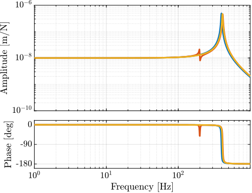
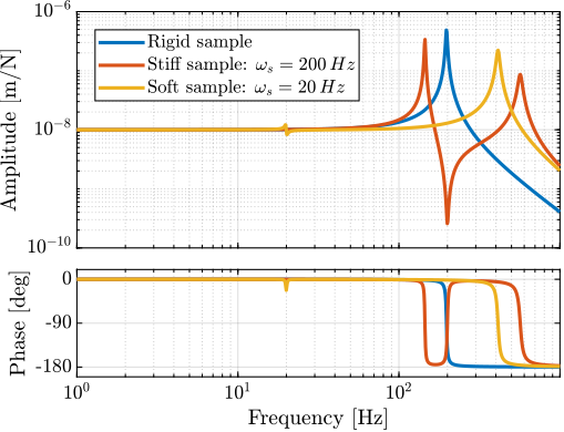
Nano Active Stabilization System - Uniaxial Model
- Glossary and Acronyms - Tables
- Introduction
- Micro Station Model
- Nano-Hexapod Model
- Disturbance Identification
- Open-Loop Dynamic Noise Budgeting
- Active Damping
- Position Feedback Controller
- Effect of limited micro-station compliance
- Effect of Payload Dynamics
- Conclusion
- Bibliography
- Glossary
- Footnotes
This report is also available as a pdf.
Glossary and Acronyms - Tables ignore
| label | name | description |
|---|---|---|
| ms | \ensuremath{m_s} | Mass of the sample |
| mn | \ensuremath{m_n} | Mass of the nano-hexapod |
| mh | \ensuremath{m_h} | Mass of the micro-hexapod |
| mt | \ensuremath{m_t} | Mass of the micro-station stages |
| mg | \ensuremath{m_g} | Mass of the granite |
| xf | \ensuremath{x_f} | Floor motion |
| ft | \ensuremath{f_t} | Disturbance force of the micro-station |
| fs | \ensuremath{f_s} | Direct forces applied on the sample |
| d | \ensuremath{d} | Measured motion between the nano-hexapod and the granite |
| fn | \ensuremath{f_n} | Force sensor on the nano-hexapod |
| psdx | \ensuremath{Φx} | Power spectral density of signal $x$ |
| asdx | \ensuremath{Γx} | Amplitude spectral density of signal $x$ |
| cpsx | \ensuremath{Φx} | Cumulative Power Spectrum of signal $x$ |
| casx | \ensuremath{Γx} | Cumulative Amplitude Spectrum of signal $x$ |
| key | abbreviation | full form |
|---|---|---|
| haclac | HAC-LAC | High Authority Control - Low Authority Control |
| hac | HAC | High Authority Control |
| lac | LAC | Low Authority Control |
| nass | NASS | Nano Active Stabilization System |
| asd | ASD | Amplitude Spectral Density |
| psd | PSD | Power Spectral Density |
| cps | CPS | Cumulative Power Spectrum |
| cas | CAS | Cumulative Amplitude Spectrum |
| frf | FRF | Frequency Response Function |
| iff | IFF | Integral Force Feedback |
| rdc | RDC | Relative Damping Control |
Introduction ignore
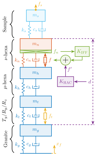
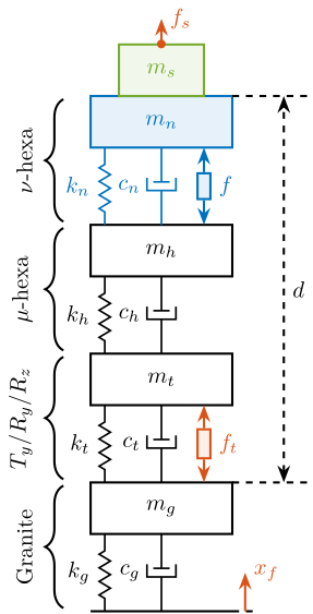
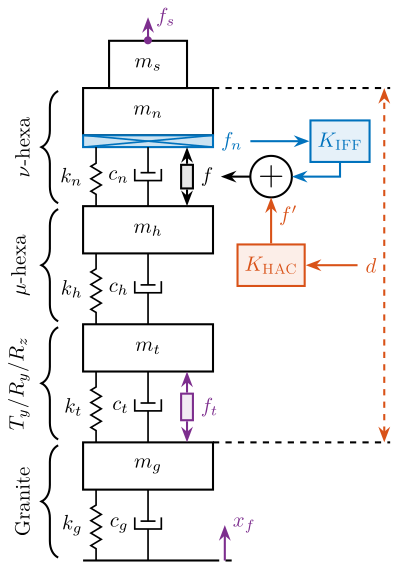
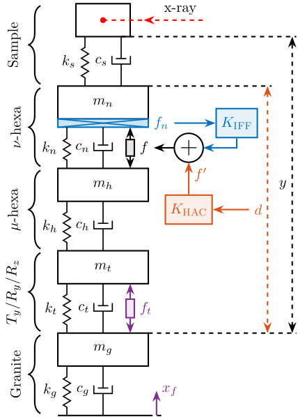
In this report, a uniaxial model of the acrfull:nass is developed and used to obtain a first idea of the challenges involved in this complex system. Note that in this study, only the vertical direction is considered (which is the most stiff), but other directions were considered as well, yielding to similar conclusions. The model is schematically shown in Figure ref:fig:uniaxial_overview_model_sections where the colors represent the parts studied in different sections.
To have a relevant model, the micro-station dynamics is first identified and its model is tuned to match the measurements (Section ref:sec:micro_station_model). Then, a model of the nano-hexapod is added on top of the micro-station. With the added sample and sensors, this gives a uniaxial dynamical model of the acrshort:nass that will be used for further analysis (Section ref:sec:nano_station_model).
The disturbances affecting position stability are identified experimentally (Section ref:sec:uniaxial_disturbances) and included in the model for dynamical noise budgeting (Section ref:sec:uniaxial_noise_budgeting). In all the following analysis, three nano-hexapod stiffnesses are considered to better understand the trade-offs and to find the most adequate nano-hexapod design. Three sample masses are also considered to verify the robustness of the applied control strategies with respect to a change of sample.
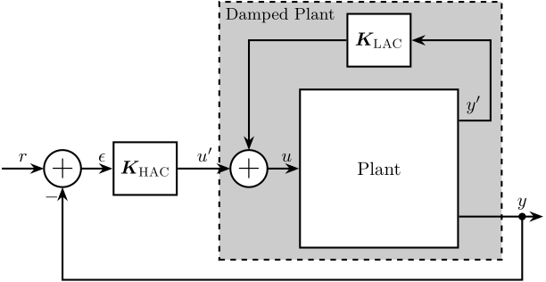
To improve the position stability of the sample, an acrfull:haclac strategy is applied. It consists of first actively damping the plant (the acrshort:lac part), and then applying a position control on the damped plant (the acrshort:hac part).
Three active damping techniques are studied (Section ref:sec:uniaxial_active_damping) which are used to both reduce the effect of disturbances and make the system easier to control afterwards. Once the system is well damped, a feedback position controller is applied and the obtained performance is analyzed (Section ref:sec:uniaxial_position_control).
Two key effects that may limit that positioning performances are then considered: the limited micro-station compliance (Section ref:sec:uniaxial_support_compliance) and the presence of dynamics between the nano-hexapod and the sample's point of interest (Section ref:sec:uniaxial_payload_dynamics).
\begin{tikzpicture}
  % ====================
  % Parameters
  % ====================
  \def\massw{2.2}  % Width of the masses
  \def\massh{0.8}  % Height of the masses
  \def\spaceh{1.2} % Height of the springs/dampers
  \def\dispw{0.4}  % Width of the dashed line for the displacement
  \def\disph{0.3}  % Height of the arrow for the displacements
  \def\bracs{0.05} % Brace spacing vertically
  \def\brach{-12pt} % Brace shift horizontaly
  \def\fsensh{0.2} % Height of the force sensor
  \def\velsize{0.2} % Size of the velocity sensor
  % ====================

  % IFF
  % ====================
  % Ground
  % ====================
  \draw[draw=colorblue] (-0.5*\massw, 0) -- (0.5*\massw, 0);
  \draw[dashed,draw=coloryellow] (0.5*\massw, 0) -- ++(\dispw, 0);
  \draw[->, color=coloryellow] (0.5*\massw+0.5*\dispw, 0) -- ++(0, 2*\disph) node[right, color=coloryellow]{$x_{f}$};
  % ====================

  % ====================
  % Granite
  \begin{scope}[shift={(0, 0)}]
    % Mass
    \draw[draw=colorblue,fill=colorblue!10!white] (-0.5*\massw, \spaceh) rectangle (0.5*\massw, \spaceh+\massh) node[pos=0.5,color=colorblue]{$m_{g}$};

    % Spring, Damper, and Actuator
    \draw[spring,draw=colorblue]  (-0.4*\massw, 0) -- (-0.4*\massw, \spaceh) node[midway, left=0.1, color=colorblue]{$k_{g}$};
    \draw[damper={colorblue}{}{}] (0, 0)           -- ( 0, \spaceh)          node[midway, left=0.2, color=colorblue]{$c_{g}$};

    % Legend
    \draw[decorate, decoration={brace, amplitude=8pt}, xshift=\brach] %
    (-0.5*\massw, \bracs) -- (-0.5*\massw, \spaceh+\massh-\bracs) node[midway,rotate=90,anchor=south,yshift=10pt]{Granite};

    % Displacements
    \draw[dashed, draw=colorpurple] (0.5*\massw, \spaceh+\massh) -- ++(7.5*\dispw, 0) coordinate(xg);
  \end{scope}
  % ====================


  % ====================
  % Stages
  \begin{scope}[shift={(0, \spaceh+\massh)}]
    % Mass
    \draw[draw=colorblue,fill=colorblue!10!white] (-0.5*\massw, \spaceh) rectangle (0.5*\massw, \spaceh+\massh) node[pos=0.5,color=colorblue]{$m_{t}$};

    % Spring, Damper, and Actuator
    \draw[spring,draw=colorblue]  (-0.4*\massw, 0) -- (-0.4*\massw, \spaceh) node[midway, left=0.1,color=colorblue]{$k_{t}$};
    \draw[damper={colorblue}{}{}] (0, 0)           -- ( 0, \spaceh)          node[midway, left=0.2,color=colorblue]{$c_{t}$};

    % Disturbance
    \draw[actuator={0.45}{0.2}{coloryellow}] ( 0.3*\massw, 0) -- (0.3*\massw, \spaceh) node[midway, right=0.1, color=coloryellow](ft){$f_{t}$};

    % Legend
    \draw[decorate, decoration={brace, amplitude=8pt}, xshift=\brach] %
    (-0.5*\massw, \bracs) -- (-0.5*\massw, \spaceh+\massh-\bracs) node[midway,rotate=90,anchor=south,yshift=10pt]{$T_y$/$R_y$/$R_z$};
  \end{scope}
  % ====================


  % ====================
  % Hexapod
  \begin{scope}[shift={(0, 2*(\spaceh+\massh))}]
    % Mass
    \draw[draw=colorblue,fill=colorblue!10!white] (-0.5*\massw, \spaceh) rectangle (0.5*\massw, \spaceh+\massh) node[pos=0.5,color=colorblue]{$m_h$};

    % Spring, Damper, and Actuator
    \draw[spring,draw=colorblue]  (-0.4*\massw, 0) -- (-0.4*\massw, \spaceh) node[midway, left=0.1,color=colorblue]{$k_h$};
    \draw[damper={colorblue}{}{}] (0, 0)           -- ( 0, \spaceh)          node[midway, left=0.2,color=colorblue]{$c_h$};

    % Legend
    \draw[decorate, decoration={brace, amplitude=8pt}, xshift=\brach] %
    (-0.5*\massw, \bracs) -- (-0.5*\massw, \spaceh+\massh-\bracs) node[midway,rotate=90,anchor=south,yshift=10pt]{$\mu\text{-hexa}$};
  \end{scope}
  % ====================


  % ====================
  % NASS
  \begin{scope}[shift={(0, 3*(\spaceh+\massh))}]
    % Mass
    \draw[draw=colorred,fill=colorred!10!white] (-0.5*\massw, \spaceh) rectangle (0.5*\massw, \spaceh+\massh) node[pos=0.5,color=colorred]{$m_{n}$};

    % Force Sensor
    \node[forcesensor={\massw}{\fsensh}{colorgreen}] (fsensn) at (0, \spaceh-\fsensh){};
    \node[right, color=colorgreen] (fn) at (fsensn.east) {$f_n$};

    % Spring, Damper, and Actuator
    \draw[spring,draw=colorred]  (-0.4*\massw, 0) -- (-0.4*\massw, \spaceh-\fsensh) node[midway, left=0.1,color=colorred]{$k_{n}$};
    \draw[damper={colorred}{}{}] (0, 0)           -- ( 0, \spaceh-\fsensh)          node[midway, left=0.2,color=colorred]{$c_{n}$};
    \draw[actuator={0.4}{0.2}{colorred}] ( 0.3*\massw, 0) -- (0.3*\massw, \spaceh-\fsensh) node[midway, right=0.1,color=colorred](f){$f$};

    % Legend
    \draw[decorate, decoration={brace, amplitude=8pt}, xshift=\brach] %
    (-0.5*\massw, \bracs) -- (-0.5*\massw, \spaceh+\massh-\bracs) node[midway,rotate=90,anchor=south,yshift=10pt]{$\nu\text{-hexa}$};

    % Displacements
    \draw[dashed,draw=colorpurple] (0.5*\massw, \spaceh+\massh) -- ++(7.5*\dispw, 0) coordinate(xnpos);
  \end{scope}
  % ====================

  % ====================
  % sample
  \begin{scope}[shift={(0, 4*(\spaceh+\massh))}]
    % Mass
    \draw[draw=colorcyan,fill=colorcyan!10!white] (-0.3*\massw, \spaceh) rectangle (0.3*\massw, \spaceh+\massh) node[pos=0.5, color=colorcyan]{$m_{s}$};

    % Spring, Damper, and Actuator
    \draw[spring,draw=colorcyan] (-0.2*\massw, 0) -- (-0.2*\massw, \spaceh) node[midway, left=0.1, color=colorcyan]{$k_{s}$};
    \draw[damper={colorcyan}{}{}] ( 0.2*\massw, 0) -- ( 0.2*\massw, \spaceh) node[midway, left=0.2, color=colorcyan]{$c_{s}$};

    % Legend
    \draw[decorate, decoration={brace, amplitude=8pt}, xshift=\brach] %
    (-0.5*\massw, \bracs) -- (-0.5*\massw, \spaceh+\massh-\bracs) %
    node[midway,rotate=90,anchor=south,yshift=10pt,align=center]{Sample};

    % External Force
    \draw[->, color=coloryellow] (0, \spaceh+\massh) node[]{$\bullet$} -- ++(0, 0.5*\massh) node[right, color=coloryellow]{$f_s$};
  \end{scope}
  % ====================

  % Measured displacement
  \draw[<->, dashed, draw=colorpurple] ($(xg)+(-0.1, 0)$) -- node[left, color=colorpurple](d){$d$} ($(xnpos)+(-0.1, 0)$);

  % ====================
  % IFF Control
  \node[block={2em}{2em}, right=1.0 of fn, color=colorgreen, fill=colorgreen!10!white] (iff) {$K_{\textsc{IFF}}$};
  \node[addb, draw=colorgreen, fill=colorgreen!10!white, right=0.5 of f.east] (ctrladd) {};
  \node[block={2em}{2em}, color=colorpurple, fill=colorpurple!10!white] (Khac) at (ctrladd|-d) {$K_{\textsc{HAC}}$};

  \draw[->, draw=colorgreen] (fn.east) -- (iff.west);
  \draw[->, draw=colorgreen] (iff.south) |- (ctrladd.east);
  \draw[->, draw=colorgreen] (ctrladd.west) -- (f.east);

  \draw[->, draw=colorpurple] (d.west) -- (Khac.east);
  \draw[->, draw=colorpurple] (Khac.north) -- (ctrladd.south) node[below right, color=colorpurple]{$f^{\prime}$};
  % ====================
\end{tikzpicture}Micro Station Model
<<sec:micro_station_model>>
Introduction ignore
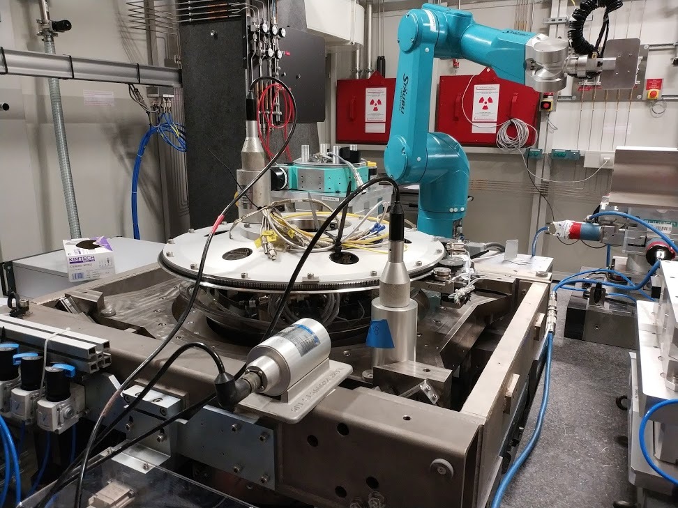
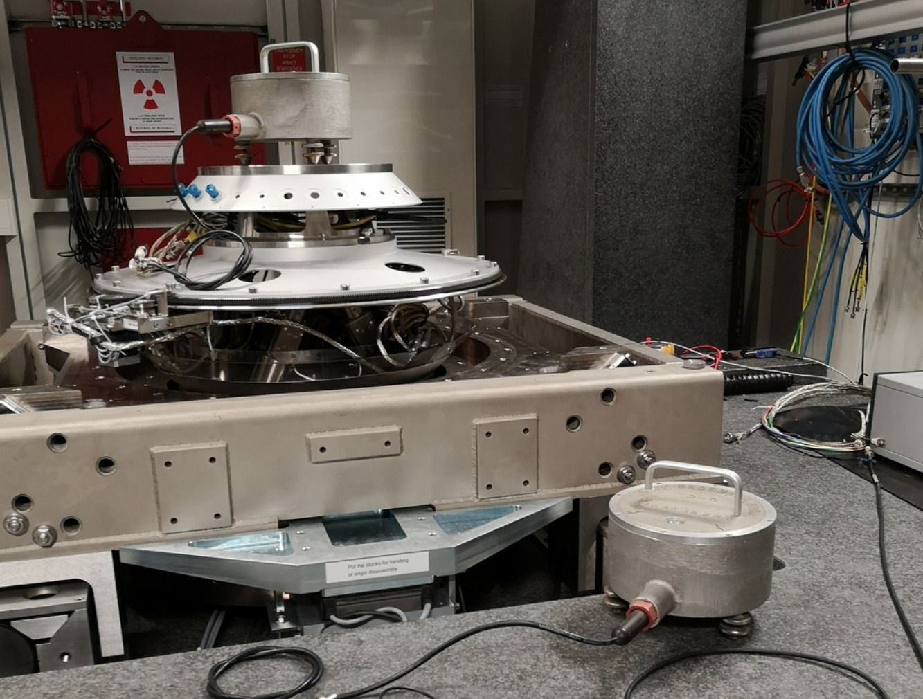
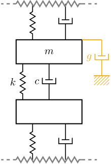
In this section, a uniaxial model of the micro-station is tuned to match measurements made on the micro-station. The measurement setup is shown in Figure ref:fig:uniaxial_ustation_first_meas_dynamics where several geophones1 are fixed to the micro-station and an instrumented hammer is used to inject forces on different stages of the micro-station.
From the measured frequency response functions (FRF), the model can be tuned to approximate the uniaxial dynamics of the micro-station.
Measured dynamics
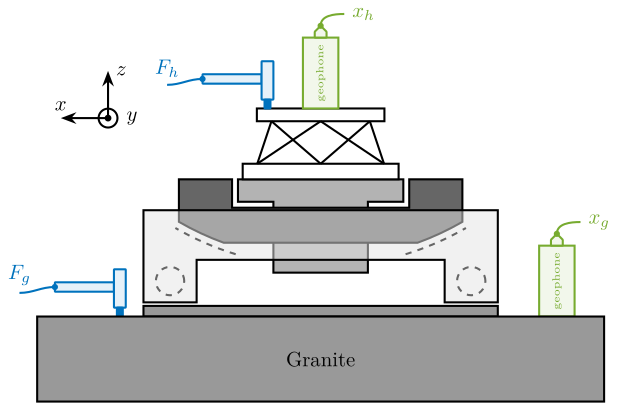
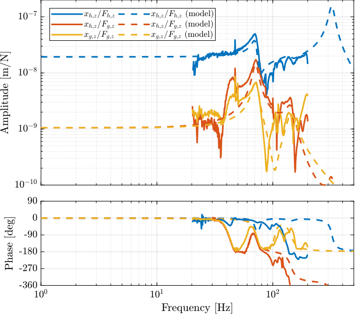
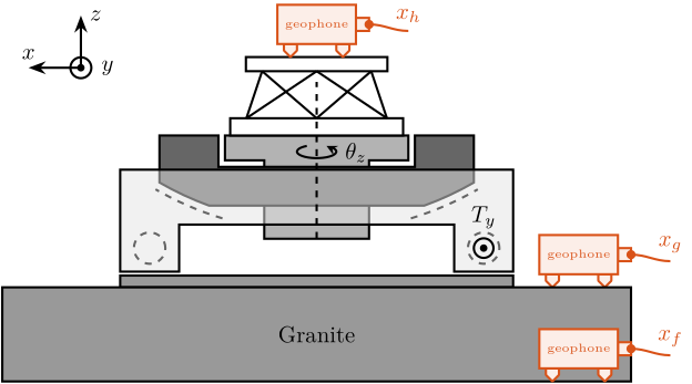
The measurement setup is schematically shown in Figure ref:fig:uniaxial_ustation_meas_dynamics_schematic where two vertical hammer hits are performed, one on the Granite (force $F_{g}$) and the other on the micro-hexapod's top platform (force $F_{h}$). The vertical inertial motion of the granite $x_{g}$ and the top platform of the micro-hexapod $x_{h}$ are measured using geophones. Three frequency response functions were computed: one from $F_{h}$ to $x_{h}$ (i.e., the compliance of the micro-station), one from $F_{g}$ to $x_{h}$ (or from $F_{h}$ to $x_{g}$) and one from $F_{g}$ to $x_{g}$.
Due to the poor coherence at low frequencies, these frequency response functions will only be shown between 20 and 200Hz (solid lines in Figure ref:fig:uniaxial_comp_frf_meas_model).
\begin{tikzpicture}
  % Parameters
  \def\blockw{6.0cm}
  \def\blockh{1.2cm}

  \def\tiltdeg{0}
  \coordinate[] (rotationpoint) at (0, 4.5*\blockh);

  \begin{scope}[rotate around={\tiltdeg:(rotationpoint)}]
    % Tilt
    \path[] ([shift=(-120:4*\blockh)]rotationpoint) coordinate(beginarc) arc (-120:-110:4*\blockh) %
    -- ([shift=(-70:4*\blockh)]rotationpoint) arc (-70:-60:4*\blockh)%
    |- ++(-0.15*\blockw, 0.6*\blockh) coordinate (spindlene)%
    |- ($(beginarc) + (0.15*\blockw, 0.2*\blockh)$) coordinate (spindlesw) -- ++(0, 0.4*\blockh) coordinate(tiltte) -| cycle;

    % Spindle
    \coordinate[] (spindlese) at (spindlesw-|spindlene);
    \draw[fill=black!30] ($(spindlese)+(-0.1,0.1)+(-0.1*\blockw, 0)$) -| ($(spindlene)+(-0.1, 0)$) -| coordinate[pos=0.25](spindletop) ($(spindlesw)+(0.1,0.1)$) -| ++(0.1*\blockw, -\blockh) -| coordinate[pos=0.25](spindlebot) cycle;

    % \draw[dashed, color=black!60] ($(spindletop)+(0, 0.2)$) -- ($(spindlebot)+(0,-0.2)$);

    % Tilt
    \draw[fill=black!60] ([shift=(-120:4*\blockh)]rotationpoint) coordinate(beginarc) arc (-120:-110:4*\blockh) %
    -- ([shift=(-70:4*\blockh)]rotationpoint) arc (-70:-60:4*\blockh)%
    |- coordinate (tiltne) ++(-0.15*\blockw, 0.6*\blockh) coordinate (spindlene)%
    |- ($(beginarc) + (0.15*\blockw, 0.2*\blockh)$) coordinate (spindlesw) -- ++(0, 0.4*\blockh) -| cycle;

    % Micro-Hexapod
    \begin{scope}[shift={(spindletop)}]
      % Parameters definitions
      \def\baseh{0.22*\blockh} % Height of the base
      \def\naceh{0.18*\blockh} % Height of the nacelle
      \def\baser{0.22*\blockw} % Radius of the base
      \def\nacer{0.18*\blockw} % Radius of the nacelle

      \def\armr{0.2*\blockh} % Radius of the arms
      \def\basearmborder{0.2}
      \def\nacearmborder{0.2}

      \def\xnace{0} \def\ynace{\blockh-\naceh} \def\anace{0}
      \def\xbase{0} \def\ybase{0} \def\abase{0}

      % Hexapod1
      \begin{scope}[shift={(\xbase, \ybase)}, rotate=\abase]
        % Base
        \draw[fill=white] (-\baser, 0) coordinate[](uhexabot) rectangle (\baser, \baseh);

        \coordinate[] (armbasel) at (-\baser+\basearmborder+\armr, \baseh);
        \coordinate[] (armbasec) at (0, \baseh);
        \coordinate[] (armbaser) at (\baser-\basearmborder-\armr, \baseh);

        \begin{scope}[shift={(\xnace, \ynace)}, rotate=\anace]
          \draw[fill=white] (-\nacer, 0) rectangle (\nacer, \naceh);
          \coordinate[] (uhexatop) at (0, \naceh);
          \coordinate[] (armnacel) at (-\nacer+\nacearmborder+\armr, 0);
          \coordinate[] (armnacec) at (0, 0);
          \coordinate[] (armnacer) at (\nacer-\nacearmborder-\armr, 0);
        \end{scope}

        \draw[] (armbasec) -- (armnacer);
        \draw[] (armbasec) -- (armnacel);
        \draw[] (armbasel) -- coordinate(mhexaw) (armnacel);
        \draw[] (armbasel) -- (armnacec);
        \draw[] (armbaser) -- (armnacec);
        \draw[] (armbaser) -- coordinate(mhexae) (armnacer);
      \end{scope}
    \end{scope}

    \begin{scope}[shift={(uhexatop)}] % Geophone - Hexapod
      \draw[draw=colorgreen, fill=colorgreen!10!white] (-0.3, 0) rectangle node[midway, color=colorgreen, rotate=90]{\tiny geophone} (0.3, 1.2);
      \draw[rounded corners=0.1, draw=colorgreen, fill=colorgreen!10!white] (-0.1, 1.2) -- ++(0, 0.1) -- ++(0.1, 0.1) -- ++(0.1, -0.1) -- ++(0, -0.1) --cycle;
      \node[fill,shape=circle,minimum size=3pt,inner sep=0pt, color=colorgreen] at (0, 1.4){};
      \draw[out=90, in=180, draw=colorgreen] (0, 1.4) to ++(0.4, 0.2) node[right, color=colorgreen]{$x_{h}$};
    \end{scope}

    \begin{scope}[shift={(uhexatop)}] % Instrumented Hammer - Hexapod
      \begin{scope}[shift={(-1.5, 0)}]
        \draw[fill=white, rounded corners=0.2, draw=colorblue, fill=colorblue!10!white] (-0.5, 0.42) rectangle (0.5, 0.58);
        \draw[fill=white, rounded corners=0.2, draw=colorblue, fill=colorblue!10!white] (0.5, 0.15) rectangle (0.7, 0.8);
        \draw[fill=white, rounded corners=0.2, color=colorblue] (0.55, 0.15) rectangle (0.65, 0);
        \draw[out=180, in=0, draw=colorblue] (-0.5, 0.5) to ++(-0.6, -0.1) node[above, color=colorblue]{$F_{h}$};
        \node[fill,shape=circle,minimum size=3pt,inner sep=0pt, color=colorblue] at (-0.5, 0.5){};
      \end{scope}
    \end{scope}
  \end{scope}

  \begin{scope}[shift={(0, -0.3*\blockh)}]
    % Translation Stage - fixed part
    \draw[fill=black!40] (-0.5*\blockw, 0) coordinate[](tyb) rectangle (0.5*\blockw, 0.15*\blockh);
    \coordinate[] (measposbot) at (0.5*\blockw, 0);

    % Translation Stage - mobile part
    \draw[fill=black!10, fill opacity=0.5] (-0.5*\blockw, 0.2*\blockh) -- (-0.5*\blockw, 1.5*\blockh) coordinate[](tyt) -- (0.5*\blockw, 1.5*\blockh) -- (0.5*\blockw, 0.2*\blockh) -- (0.35*\blockw, 0.2*\blockh) -- (0.35*\blockw, 0.8*\blockh) -- (-0.35*\blockw, 0.8*\blockh) -- (-0.35*\blockw, 0.2*\blockh) -- cycle;

    % Translation Guidance
    \draw[dashed, color=black!60] ($(-0.5*\blockw, 0)+( 0.075*\blockw,0.5*\blockh)$) circle (0.2*\blockh);
    \draw[dashed, color=black!60] ($( 0.5*\blockw, 0)+(-0.075*\blockw,0.5*\blockh)$) circle (0.2*\blockh);

    % \draw[fill, color=black] ($( 0.5*\blockw, 0)+(-0.075*\blockw,0.5*\blockh)$) circle (0.04);
    % \node[draw, circle, inner sep=0pt, minimum size=0.3cm, label=above:$T_y$] at ($( 0.5*\blockw, 0)+(-0.075*\blockw,0.5*\blockh)$){};

    % Tilt Guidance
    \draw[dashed, color=black!60] ([shift=(-107:4.1*\blockh)]rotationpoint) arc (-107:-120:4.1*\blockh);
    \draw[dashed, color=black!60] ([shift=( -73:4.1*\blockh)]rotationpoint) arc (-73:-60:4.1*\blockh);

    \begin{scope}[shift={(4.0, 0)}] % Geophone - Granite
      \draw[draw=colorgreen, fill=colorgreen!10!white] (-0.3, 0) rectangle node[midway, color=colorgreen, rotate=90]{\tiny geophone} (0.3, 1.2);
      \draw[rounded corners=0.1, draw=colorgreen, fill=colorgreen!10!white] (-0.1, 1.2) -- ++(0, 0.1) -- ++(0.1, 0.1) -- ++(0.1, -0.1) -- ++(0, -0.1) --cycle;
      \node[fill,shape=circle,minimum size=3pt,inner sep=0pt, color=colorgreen] at (0, 1.4){};
      \draw[out=90, in=180, draw=colorgreen] (0, 1.4) to ++(0.4, 0.2) node[right, color=colorgreen]{$x_{g}$};
    \end{scope}

    \begin{scope}[shift={(-4.0, 0)}] % Instrumented Hammer - Granite
      \draw[fill=white, rounded corners=0.2, draw=colorblue, fill=colorblue!10!white] (-0.5, 0.42) rectangle (0.5, 0.58);
      \draw[fill=white, rounded corners=0.2, draw=colorblue, fill=colorblue!10!white] (0.5, 0.15) rectangle (0.7, 0.8);
      \draw[fill=white, rounded corners=0.2, color=colorblue] (0.55, 0.15) rectangle (0.65, 0);
      \draw[out=180, in=0, draw=colorblue] (-0.5, 0.5) to ++(-0.6, -0.1) node[above, color=colorblue]{$F_{g}$};
      \node[fill,shape=circle,minimum size=3pt,inner sep=0pt, color=colorblue] at (-0.5, 0.5){};
    \end{scope}
  \end{scope}

  % Granite
  \draw[fill=black!40] (-0.8*\blockw, -0.3*\blockh) rectangle node[midway]{Granite} (0.8*\blockw, -1.5*\blockh);

  % Vertical line
  % \draw[dashed, color=black] (spindlebot) -- ++(0, 2*\blockh);
  % \node[] at ($(spindlebot)+(0, 1.1*\blockh)$) {\AxisRotator[rotate=-90]};
  % \node[right, shift={(0.3,0)}] at ($(spindlebot)+(0, 1.1*\blockh)$) {$\theta_z$};

  % Axis
  \begin{scope}[shift={(-0.6*\blockw, 2.5*\blockh)}]
    \def\axissize{0.8cm}
    \draw[->] (0, 0) -- ++(0, \axissize) node[right]{$z$};
    \draw[->] (0, 0) -- ++(-\axissize, 0) node[above]{$x$};
    \draw[fill, color=black] (0, 0) circle (0.05*\axissize);
    \node[draw, circle, inner sep=0pt, minimum size=0.4*\axissize, label=right:$y$] (yaxis) at (0, 0){};
  \end{scope}
\end{tikzpicture}
%% Load measured FRF
load('meas_microstation_frf.mat');Uniaxial Model
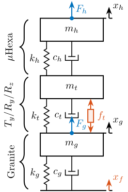
The uniaxial model of the micro-station is shown in Figure ref:fig:uniaxial_model_micro_station. It consists of a mass spring damper system with three degrees of freedom. A mass-spring-damper system represents the granite (with mass $m_g$, stiffness $k_g$ and damping $c_g$). Another mass-spring-damper system represents the different micro-station stages (the $T_y$ stage, the $R_y$ stage and the $R_z$ stage) with mass $m_t$, damping $c_t$ and stiffness $k_t$. Finally, a third mass-spring-damper system represents the micro-hexapod with mass $m_h$, damping $c_h$ and stiffness $k_h$.
The masses of the different stages are estimated from the 3D model, while the stiffnesses are from the data-sheet of the manufacturers. The damping coefficients were tuned to match the damping identified from the measurements. The parameters obtained are summarized in Table ref:tab:uniaxial_ustation_parameters.
| Stage | Mass | Stiffness | Damping |
|---|---|---|---|
| Micro-Hexapod | $m_h = 15\,\text{kg}$ | $k_h = 61\,N/\mu m$ | $c_h = 3\,\frac{kN}{m/s}$ |
| $T_y$, $R_y$, $R_z$ | $m_t = 1200\,\text{kg}$ | $k_t = 520\,N/\mu m$ | $c_t = 80\,\frac{kN}{m/s}$ |
| Granite | $m_g = 2500\,\text{kg}$ | $k_g = 950\,N/\mu m$ | $c_g = 250\,\frac{kN}{m/s}$ |
Two disturbances are considered which are shown in red: the floor motion $x_f$ and the stage vibrations represented by $f_t$. The hammer impacts $F_{h}, F_{g}$ are shown in blue, whereas the measured inertial motions $x_{h}, x_{g}$ are shown in black.
\begin{tikzpicture}
  % ====================
  % Parameters
  % ====================
  \def\massw{2.2}  % Width of the masses
  \def\massh{0.8}  % Height of the masses
  \def\spaceh{1.2} % Height of the springs/dampers
  \def\dispw{0.4}  % Width of the dashed line for the displacement
  \def\disph{0.4}  % Height of the arrow for the displacements
  \def\bracs{0.05} % Brace spacing vertically
  \def\brach{-12pt} % Brace shift horizontaly
  \def\fsensh{0.2} % Height of the force sensor
  \def\velsize{0.2} % Size of the velocity sensor
  % ====================


  % ====================
  % Floor
  % ====================
  \draw (-0.5*\massw, 0) -- (0.5*\massw, 0);
  \draw[dashed] (0.5*\massw, 0) -- ++(\dispw, 0);
  \draw[->, draw=colorred] (0.5*\massw+0.5*\dispw, 0) -- ++(0, \disph) node[right, color=colorred]{$x_{f}$};
  % ====================

  % ====================
  % Granite
  \begin{scope}[shift={(0, 0)}]
    % Mass
    \draw[fill=white] (-0.5*\massw, \spaceh) rectangle (0.5*\massw, \spaceh+\massh) node[pos=0.5]{$m_{g}$};

    % Spring, Damper, and Actuator
    \draw[spring] (-0.4*\massw, 0) -- (-0.4*\massw, \spaceh) node[midway, left=0.1]{$k_{g}$};
    \draw[damper] (0, 0)           -- ( 0, \spaceh)          node[midway, left=0.2]{$c_{g}$};

    % Legend
    \draw[decorate, decoration={brace, amplitude=8pt}, xshift=\brach] %
    (-0.5*\massw, \bracs) -- (-0.5*\massw, \spaceh+\massh-\bracs) node[midway,rotate=90,anchor=south,yshift=10pt]{Granite};

    % Displacement
    \draw[dashed] (0.5*\massw, \spaceh+\massh) -- ++(\dispw, 0);
    \draw[->] (0.5*\massw+0.5*\dispw, \spaceh+\massh) -- ++(0, \disph) node[right]{$x_{g}$};
  \end{scope}
  % ====================


  % ====================
  % Stages
  \begin{scope}[shift={(0, \spaceh+\massh)}]
    % Mass
    \draw[fill=white] (-0.5*\massw, \spaceh) rectangle (0.5*\massw, \spaceh+\massh) node[pos=0.5]{$m_{t}$};

    % Spring, Damper, and Actuator
    \draw[spring] (-0.4*\massw, 0) -- (-0.4*\massw, \spaceh) node[midway, left=0.1]{$k_{t}$};
    \draw[damper] (0, 0)           -- ( 0, \spaceh)          node[midway, left=0.2]{$c_{t}$};

    % Disturbance
    \draw[actuator={0.45}{0.2}{colorred}] ( 0.3*\massw, 0) -- (0.3*\massw, \spaceh) node[midway, right=0.1, color=colorred](ft){$f_t$};

    % Legend
    \draw[decorate, decoration={brace, amplitude=8pt}, xshift=\brach] %
    (-0.5*\massw, \bracs) -- (-0.5*\massw, \spaceh+\massh-\bracs) node[midway,rotate=90,anchor=south,yshift=10pt]{$T_y$/$R_y$/$R_z$};

    % External Force
    \draw[->, color=colorblue] (0, 0)node[branch] -- ++(0, 1.5*\dispw) node[below right]{$F_g$};

    % % Displacement
    % \draw[dashed] (0.5*\massw, \spaceh+\massh) -- ++(\dispw, 0);
    % \draw[->] (0.5*\massw+0.5*\dispw, \spaceh+\massh) -- ++(0, \disph) node[right]{$x_{t}$};
  \end{scope}
  % ====================


  % ====================
  % Hexapod
  \begin{scope}[shift={(0, 2*(\spaceh+\massh))}]
    % Mass
    \draw[fill=white] (-0.5*\massw, \spaceh) rectangle (0.5*\massw, \spaceh+\massh) node[pos=0.5]{$m_{h}$};

    % Spring, Damper, and Actuator
    \draw[spring] (-0.4*\massw, 0) -- (-0.4*\massw, \spaceh) node[midway, left=0.1]{$k_{h}$};
    \draw[damper] (0, 0)           -- ( 0, \spaceh)          node[midway, left=0.2]{$c_{h}$};

    % Legend
    \draw[decorate, decoration={brace, amplitude=8pt}, xshift=\brach] %
    (-0.5*\massw, \bracs) -- (-0.5*\massw, \spaceh+\massh-\bracs) node[midway,rotate=90,anchor=south,yshift=10pt]{$\mu\text{Hexa}$};

    % Displacement
    \draw[dashed] (0.5*\massw, \spaceh+\massh) -- ++(\dispw, 0);
    \draw[->] (0.5*\massw+0.5*\dispw, \spaceh+\massh) -- ++(0, \disph) node[right]{$x_{h}$};

    % External Force
    \draw[->, color=colorblue] (0, \spaceh+\massh)node[branch] -- ++(0, 1.5*\dispw) node[below right]{$F_h$};
  \end{scope}
  % ====================
\end{tikzpicture}
%% Parameters - Mass
mh = 15; % Micro Hexapod [kg]
mt = 1200; % Ty + Ry + Rz [kg]
mg = 2500; % Granite [kg]%% Parameters - Stiffnesses
kh = 6.11e+07; % [N/m]
kt = 5.19e+08; % [N/m]
kg = 9.50e+08; % [N/m]%% Parameters - damping
ch = 2*0.05*sqrt(kh*mh); % [N/(m/s)]
ct = 2*0.05*sqrt(kt*mt); % [N/(m/s)]
cg = 2*0.08*sqrt(kg*mg); % [N/(m/s)]Comparison of model and measurements
The transfer functions from the forces injected by the hammers to the measured inertial motion of the micro-hexapod and granite are extracted from the uniaxial model and compared to the measurements in Figure ref:fig:uniaxial_comp_frf_meas_model.
Because the uniaxial model has three degrees of freedom, only three modes with frequencies at $70\,\text{Hz}$, $140\,\text{Hz}$ and $320\,\text{Hz}$ are modeled. Many more modes can be observed in the measurements (see Figure ref:fig:uniaxial_comp_frf_meas_model). However, the goal is not to have a perfect match with the measurement (this would require a much more complex model), but to have a first approximation. More accurate models will be used later on.
Nano-Hexapod Model
<<sec:nano_station_model>>
Introduction ignore
A model of the nano-hexapod and sample is now added on top of the uniaxial model of the micro-station (Figure ref:fig:uniaxial_model_micro_station_nass). Disturbances (shown in red) are gls:fs the direct forces applied to the sample (for example cable forces), gls:ft representing the vibrations induced when scanning the different stages and gls:xf the floor motion. The control signal is the force applied by the nano-hexapod $f$ and the measurement is the relative motion between the sample and the granite $d$. The sample is here considered as a rigid body and rigidly fixed to the nano-hexapod. The effect of resonances between the sample's point of interest and the nano-hexapod actuator will be considered in Section ref:sec:uniaxial_payload_dynamics.
\begin{tikzpicture}
  % ====================
  % Parameters
  % ====================
  \def\massw{2.2}  % Width of the masses
  \def\massh{0.8}  % Height of the masses
  \def\spaceh{1.2} % Height of the springs/dampers
  \def\dispw{0.4}  % Width of the dashed line for the displacement
  \def\disph{0.3}  % Height of the arrow for the displacements
  \def\bracs{0.05} % Brace spacing vertically
  \def\brach{-12pt} % Brace shift horizontaly
  \def\fsensh{0.2} % Height of the force sensor
  \def\velsize{0.2} % Size of the velocity sensor
  % ====================

  % ====================
  % Ground
  % ====================
  \draw (-0.5*\massw, 0) -- (0.5*\massw, 0);
  \draw[dashed] (0.5*\massw, 0) -- ++(\dispw, 0);
  \draw[->, color=colorred] (0.5*\massw+0.5*\dispw, 0) -- ++(0, 2*\disph) node[right, color=colorred]{$x_{f}$};
  % ====================

  % ====================
  % Marble
  \begin{scope}[shift={(0, 0)}]
    % Mass
    \draw[fill=white] (-0.5*\massw, \spaceh) rectangle (0.5*\massw, \spaceh+\massh) node[pos=0.5]{$m_{g}$};

    % Spring, Damper, and Actuator
    \draw[spring] (-0.4*\massw, 0) -- (-0.4*\massw, \spaceh) node[midway, left=0.1]{$k_{g}$};
    \draw[damper] (0, 0)           -- ( 0, \spaceh)          node[midway, left=0.2]{$c_{g}$};

    % Legend
    \draw[decorate, decoration={brace, amplitude=8pt}, xshift=\brach] %
    (-0.5*\massw, \bracs) -- (-0.5*\massw, \spaceh+\massh-\bracs) node[midway,rotate=90,anchor=south,yshift=10pt]{Granite};

    % Displacements
    \draw[dashed] (0.5*\massw, \spaceh+\massh) -- ++(2*\dispw, 0) coordinate(xm) -- ++(\dispw, 0) coordinate(dbot);
  \end{scope}
  % ====================


  % ====================
  % Stages
  \begin{scope}[shift={(0, \spaceh+\massh)}]
    % Mass
    \draw[fill=white] (-0.5*\massw, \spaceh) rectangle (0.5*\massw, \spaceh+\massh) node[pos=0.5]{$m_{t}$};

    % % Spring, Damper, and Actuator
    \draw[spring] (-0.4*\massw, 0) -- (-0.4*\massw, \spaceh) node[midway, left=0.1]{$k_{t}$};
    \draw[damper] (0, 0)           -- ( 0, \spaceh)          node[midway, left=0.2]{$c_{t}$};
    \draw[actuator={0.45}{0.2}{colorred}] ( 0.3*\massw, 0) -- (0.3*\massw, \spaceh) node[midway, right=0.1, color=colorred](ft){$f_{t}$};

    Legend
    \draw[decorate, decoration={brace, amplitude=8pt}, xshift=\brach] %
    (-0.5*\massw, \bracs) -- (-0.5*\massw, \spaceh+\massh-\bracs) node[midway,rotate=90,anchor=south,yshift=10pt]{$T_y$/$R_y$/$R_z$};
  \end{scope}
  % ====================


  % ====================
  % Hexapod
  \begin{scope}[shift={(0, 2*(\spaceh+\massh))}]
    % Mass
    \draw[fill=white] (-0.5*\massw, \spaceh) rectangle (0.5*\massw, \spaceh+\massh) node[pos=0.5]{$m_{h}$};

    % Spring, Damper, and Actuator
    \draw[spring] (-0.4*\massw, 0) -- (-0.4*\massw, \spaceh) node[midway, left=0.1]{$k_{h}$};
    \draw[damper] (0, 0)           -- ( 0, \spaceh)          node[midway, left=0.2]{$c_{h}$};

    % Legend
    \draw[decorate, decoration={brace, amplitude=8pt}, xshift=\brach] %
    (-0.5*\massw, \bracs) -- (-0.5*\massw, \spaceh+\massh-\bracs) node[midway,rotate=90,anchor=south,yshift=10pt]{$\mu\text{-hexa}$};
  \end{scope}
  % ====================


  % ====================
  % NASS
  \begin{scope}[shift={(0, 3*(\spaceh+\massh))}]
    % Mass
    \draw[fill=colorblue!10!white, draw=colorblue] (-0.5*\massw, \spaceh) rectangle (0.5*\massw, \spaceh+\massh) node[pos=0.5,color=colorblue]{$m_{n}$};

    % Spring, Damper, and Actuator
    \draw[spring, draw=colorblue] (-0.4*\massw, 0) -- (-0.4*\massw, \spaceh) node[midway, left=0.1, color=colorblue]{$k_{n}$};
    \draw[damper={colorblue}{}{}] (0, 0)           -- ( 0, \spaceh)          node[midway, left=0.2, color=colorblue]{$c_{n}$};
    \draw[actuator={0.4}{0.2}{colorblue}] ( 0.3*\massw, 0) -- (0.3*\massw, \spaceh) node[midway, right=0.1, color=colorblue](F){$f$};

    % Displacements
    \draw[dashed] (0.5*\massw, \spaceh+\massh) -- ++(2*\dispw, 0) coordinate(xn) -- ++(\dispw, 0) coordinate(drtop);

    % Legend
    \draw[decorate, decoration={brace, amplitude=8pt}, xshift=\brach] %
    (-0.5*\massw, \bracs) -- (-0.5*\massw, \spaceh+\massh-\bracs) node[midway,rotate=90,anchor=south,yshift=10pt]{$\nu\text{-hexa}$};
  \end{scope}
  % ====================

  % ====================
  % sample
  \begin{scope}[shift={(0, 4*(\spaceh+\massh))}]
    % Mass
    \draw[fill=colorgreen!10!white, draw=colorgreen] (-0.3*\massw, 0) rectangle (0.3*\massw, \massh) node[pos=0.5,color=colorgreen]{$m_{s}$};

    % External Force
    \draw[->, color=colorred] (0, \massh) node[]{$\bullet$} -- ++(0, 0.5*\massh) node[right, color=colorred]{$f_s$};
  \end{scope}
  % ====================


  % ====================
  % Measured Displacement
  \draw[<->, dashed] (xm) -- node[midway, right]{$d$} (xn);
  % ====================
\end{tikzpicture}
Nano-Hexapod Parameters
The nano-hexapod is represented by a mass spring damper system (shown in blue in Figure ref:fig:uniaxial_model_micro_station_nass). Its mass gls:mn is set to $15\,\text{kg}$ while its stiffness $k_n$ can vary depending on the chosen architecture/technology. The sample is represented by a mass gls:ms that can vary from $1\,\text{kg}$ up to $50\,\text{kg}$.
As a first example, the nano-hexapod stiffness of is set at $k_n = 10\,N/\mu m$ and the sample mass is chosen at $m_s = 10\,\text{kg}$.
%% Nano-Hexapod Parameters
mn = 15; % [kg]
kn = 1e7; % [N/m]
cn = 2*0.01*sqrt(mn*kn); % [N/(m/s)]

%% Sample Mass
ms = 10; % [kg]
Obtained Dynamic Response
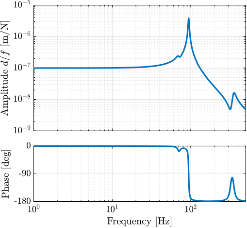
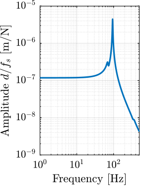
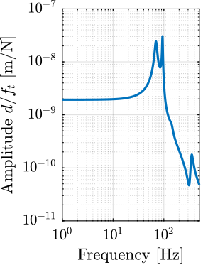
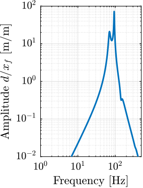
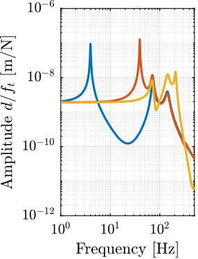
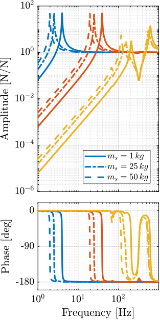
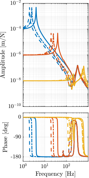
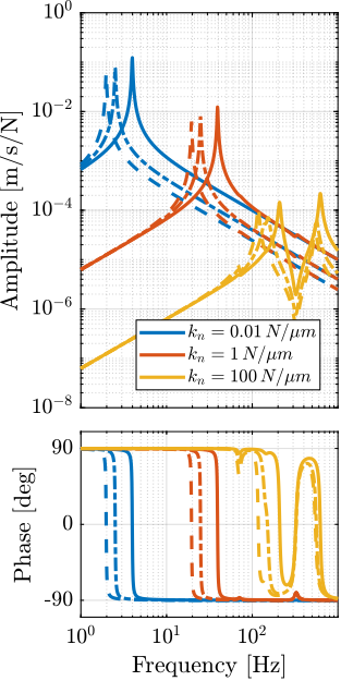
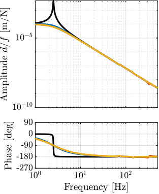
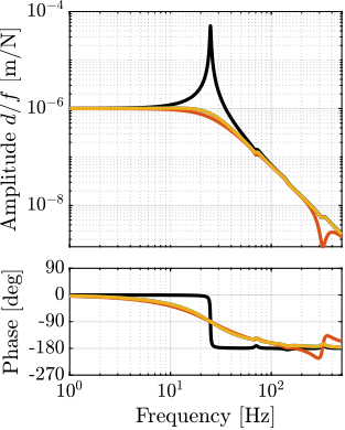
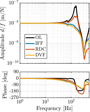
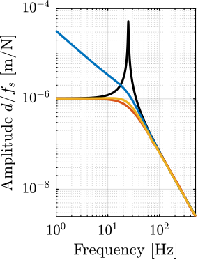
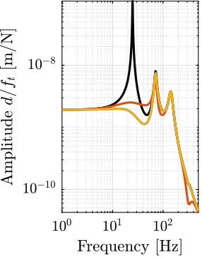
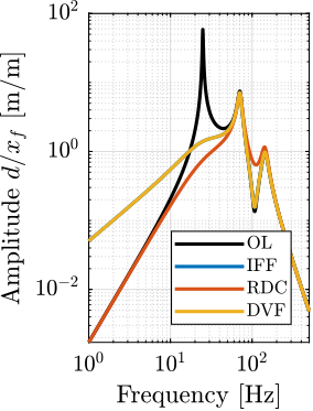
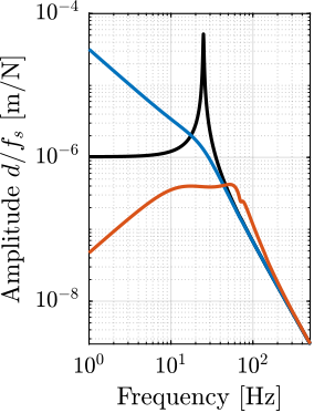
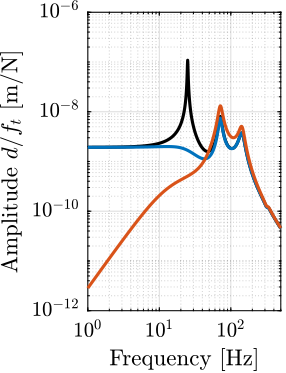
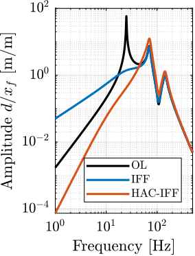
The sensitivity to disturbances (i.e., the transfer functions from $x_f,f_t,f_s$ to $d$) can be extracted from the uniaxial model of Figure ref:fig:uniaxial_model_micro_station_nass and are shown in Figure ref:fig:uniaxial_sensitivity_dist_first_params. The plant (i.e., the transfer function from actuator force $f$ to measured displacement $d$) is shown in Figure ref:fig:uniaxial_plant_first_params.
For further analysis, 9 "configurations" of the uniaxial NASS model of Figure ref:fig:uniaxial_model_micro_station_nass will be considered: three nano-hexapod stiffnesses ($k_n = 0.01\,N/\mu m$, $k_n = 1\,N/\mu m$ and $k_n = 100\,N/\mu m$) combined with three sample's masses ($m_s = 1\,kg$, $m_s = 25\,kg$ and $m_s = 50\,kg$).
Disturbance Identification
<<sec:uniaxial_disturbances>>
Introduction ignore
To quantify disturbances (red signals in Figure ref:fig:uniaxial_model_micro_station_nass), three geophones2 are used. One is located on the floor, another one on the granite, and the last one on the micro-hexapod's top platform (see Figure ref:fig:uniaxial_ustation_meas_disturbances). The geophone located on the floor was used to measure the floor motion $x_f$ while the other two geophones were used to measure vibrations introduced by scanning of the $T_y$ stage and $R_z$ stage (see Figure ref:fig:uniaxial_ustation_dynamical_id_setup).
\begin{tikzpicture}
  % Parameters
  \def\blockw{6.0cm}
  \def\blockh{1.2cm}

  \def\tiltdeg{0}
  \coordinate[] (rotationpoint) at (0, 4.5*\blockh);

  \begin{scope}[rotate around={\tiltdeg:(rotationpoint)}]
    % Tilt
    \path[] ([shift=(-120:4*\blockh)]rotationpoint) coordinate(beginarc) arc (-120:-110:4*\blockh) %
    -- ([shift=(-70:4*\blockh)]rotationpoint) arc (-70:-60:4*\blockh)%
    |- ++(-0.15*\blockw, 0.6*\blockh) coordinate (spindlene)%
    |- ($(beginarc) + (0.15*\blockw, 0.2*\blockh)$) coordinate (spindlesw) -- ++(0, 0.4*\blockh) coordinate(tiltte) -| cycle;

    % Spindle
    \coordinate[] (spindlese) at (spindlesw-|spindlene);
    \draw[fill=black!30] ($(spindlese)+(-0.1,0.1)+(-0.1*\blockw, 0)$) -| ($(spindlene)+(-0.1, 0)$) -| coordinate[pos=0.25](spindletop) ($(spindlesw)+(0.1,0.1)$) -| ++(0.1*\blockw, -\blockh) -| coordinate[pos=0.25](spindlebot) cycle;

    % \draw[dashed, color=black!60] ($(spindletop)+(0, 0.2)$) -- ($(spindlebot)+(0,-0.2)$);

    % Tilt
    \draw[fill=black!60] ([shift=(-120:4*\blockh)]rotationpoint) coordinate(beginarc) arc (-120:-110:4*\blockh) %
    -- ([shift=(-70:4*\blockh)]rotationpoint) arc (-70:-60:4*\blockh)%
    |- coordinate (tiltne) ++(-0.15*\blockw, 0.6*\blockh) coordinate (spindlene)%
    |- ($(beginarc) + (0.15*\blockw, 0.2*\blockh)$) coordinate (spindlesw) -- ++(0, 0.4*\blockh) -| cycle;

    % Micro-Hexapod
    \begin{scope}[shift={(spindletop)}]
      % Parameters definitions
      \def\baseh{0.22*\blockh} % Height of the base
      \def\naceh{0.18*\blockh} % Height of the nacelle
      \def\baser{0.22*\blockw} % Radius of the base
      \def\nacer{0.18*\blockw} % Radius of the nacelle

      \def\armr{0.2*\blockh} % Radius of the arms
      \def\basearmborder{0.2}
      \def\nacearmborder{0.2}

      \def\xnace{0} \def\ynace{\blockh-\naceh} \def\anace{0}
      \def\xbase{0} \def\ybase{0} \def\abase{0}

      % Hexapod
      \begin{scope}[shift={(\xbase, \ybase)}, rotate=\abase]
        % Base
        \draw[fill=white] (-\baser, 0) coordinate[](uhexabot) rectangle (\baser, \baseh);

        \coordinate[] (armbasel) at (-\baser+\basearmborder+\armr, \baseh);
        \coordinate[] (armbasec) at (0, \baseh);
        \coordinate[] (armbaser) at (\baser-\basearmborder-\armr, \baseh);

        \begin{scope}[shift={(\xnace, \ynace)}, rotate=\anace]
          \draw[fill=white] (-\nacer, 0) rectangle (\nacer, \naceh);
          \coordinate[] (uhexatop) at (0, \naceh);
          \coordinate[] (armnacel) at (-\nacer+\nacearmborder+\armr, 0);
          \coordinate[] (armnacec) at (0, 0);
          \coordinate[] (armnacer) at (\nacer-\nacearmborder-\armr, 0);
        \end{scope}

        \draw[] (armbasec) -- (armnacer);
        \draw[] (armbasec) -- (armnacel);
        \draw[] (armbasel) -- coordinate(mhexaw) (armnacel);
        \draw[] (armbasel) -- (armnacec);
        \draw[] (armbaser) -- (armnacec);
        \draw[] (armbaser) -- coordinate(mhexae) (armnacer);
      \end{scope}
    \end{scope}

    \begin{scope}[shift={(uhexatop)}] % Geophone - Hexapod
      \draw[rounded corners=0.1, draw=colorred, fill=colorred!10!white] (-0.5, 0.2) -- ++(0, -0.1) -- ++(0.1, -0.1) -- ++(0.1, 0.1) -- ++(0, 0.1) --cycle;
      \draw[rounded corners=0.1, draw=colorred, fill=colorred!10!white] ( 0.3, 0.2) -- ++(0, -0.1) -- ++(0.1, -0.1) -- ++(0.1, 0.1) -- ++(0, 0.1) --cycle;
      \draw[draw=colorred, fill=colorred!10!white] (0.6, 0.4) rectangle ++(0.2, 0.2);
      \node[shape=circle,minimum size=3pt,inner sep=0pt, draw=colorred, fill=colorred] at (0.8, 0.5){};
      \draw[out=0, in=180, draw=colorred] (0.8, 0.5) to ++(0.6, -0.1) node[above, color=colorred]{$x_h$};
      \draw[draw=colorred, fill=colorred!10!white] (-0.6, 0.2) rectangle node[midway, color=colorred]{\tiny geophone} (0.6, 0.8);
    \end{scope}
  \end{scope}

  \begin{scope}[shift={(0, -0.3*\blockh)}]
    % Translation Stage - fixed part
    \draw[fill=black!40] (-0.5*\blockw, 0) coordinate[](tyb) rectangle (0.5*\blockw, 0.15*\blockh);
    \coordinate[] (measposbot) at (0.5*\blockw, 0);

    % Translation Stage - mobile part
    \draw[fill=black!10, fill opacity=0.5] (-0.5*\blockw, 0.2*\blockh) -- (-0.5*\blockw, 1.5*\blockh) coordinate[](tyt) -- (0.5*\blockw, 1.5*\blockh) -- (0.5*\blockw, 0.2*\blockh) -- (0.35*\blockw, 0.2*\blockh) -- (0.35*\blockw, 0.8*\blockh) -- (-0.35*\blockw, 0.8*\blockh) -- (-0.35*\blockw, 0.2*\blockh) -- cycle;

    % Translation Guidance
    \draw[dashed, color=black!60] ($(-0.5*\blockw, 0)+( 0.075*\blockw,0.5*\blockh)$) circle (0.2*\blockh);
    \draw[dashed, color=black!60] ($( 0.5*\blockw, 0)+(-0.075*\blockw,0.5*\blockh)$) circle (0.2*\blockh);

    \draw[fill, color=black] ($( 0.5*\blockw, 0)+(-0.075*\blockw,0.5*\blockh)$) circle (0.04);
    \node[draw, circle, inner sep=0pt, minimum size=0.3cm, label=above:$T_y$] at ($( 0.5*\blockw, 0)+(-0.075*\blockw,0.5*\blockh)$){};

    % Tilt Guidance
    \draw[dashed, color=black!60] ([shift=(-107:4.1*\blockh)]rotationpoint) arc (-107:-120:4.1*\blockh);
    \draw[dashed, color=black!60] ([shift=( -73:4.1*\blockh)]rotationpoint) arc (-73:-60:4.1*\blockh);

    \begin{scope}[shift={(4.0, 0)}] % Geophone - Granite
      \draw[rounded corners=0.1, draw=colorred, fill=colorred!10!white] (-0.5, 0.2) -- ++(0, -0.1) -- ++(0.1, -0.1) -- ++(0.1, 0.1) -- ++(0, 0.1) --cycle;
      \draw[rounded corners=0.1, draw=colorred, fill=colorred!10!white] ( 0.3, 0.2) -- ++(0, -0.1) -- ++(0.1, -0.1) -- ++(0.1, 0.1) -- ++(0, 0.1) --cycle;
      \draw[draw=colorred, fill=colorred!10!white] (0.6, 0.4) rectangle ++(0.2, 0.2);
      \node[shape=circle,minimum size=3pt,inner sep=0pt, draw=colorred, fill=colorred] at (0.8, 0.5){};
      \draw[out=0, in=180, draw=colorred] (0.8, 0.5) to ++(0.6, -0.1) node[above, color=colorred]{$x_g$};
      \draw[draw=colorred, fill=colorred!10!white] (-0.6, 0.2) rectangle node[midway, color=colorred]{\tiny geophone} (0.6, 0.8);
    \end{scope}
  \end{scope}

  % Granite
  \draw[fill=black!40] (-0.8*\blockw, -0.3*\blockh) rectangle node[midway]{Granite} (0.8*\blockw, -1.5*\blockh);

  \begin{scope}[shift={(4.0, -1.5*\blockh)}] % Geophone - Floor
    \draw[rounded corners=0.1, draw=colorred, fill=colorred!10!white] (-0.5, 0.2) -- ++(0, -0.1) -- ++(0.1, -0.1) -- ++(0.1, 0.1) -- ++(0, 0.1) --cycle;
    \draw[rounded corners=0.1, draw=colorred, fill=colorred!10!white] ( 0.3, 0.2) -- ++(0, -0.1) -- ++(0.1, -0.1) -- ++(0.1, 0.1) -- ++(0, 0.1) --cycle;
    \draw[draw=colorred, fill=colorred!10!white] (0.6, 0.4) rectangle ++(0.2, 0.2);
    \node[shape=circle,minimum size=3pt,inner sep=0pt, draw=colorred, fill=colorred] at (0.8, 0.5){};
    \draw[out=0, in=180, draw=colorred] (0.8, 0.5) to ++(0.6, -0.1) node[above, color=colorred]{$x_f$};
    \draw[draw=colorred, fill=colorred!10!white] (-0.6, 0.2) rectangle node[midway, color=colorred]{\tiny geophone} (0.6, 0.8);
  \end{scope}

  % Vertical line
  \draw[dashed, color=black] (spindlebot) -- ++(0, 2*\blockh);
  \node[] at ($(spindlebot)+(0, 1.1*\blockh)$) {\AxisRotator[rotate=-90]};
  \node[right, shift={(0.3,0)}] at ($(spindlebot)+(0, 1.1*\blockh)$) {$\theta_z$};

  % Axis
  \begin{scope}[shift={(-0.6*\blockw, 2.5*\blockh)}]
    \def\axissize{0.8cm}
    \draw[->] (0, 0) -- ++(0, \axissize) node[right]{$z$};
    \draw[->] (0, 0) -- ++(-\axissize, 0) node[above]{$x$};
    \draw[fill, color=black] (0, 0) circle (0.05*\axissize);
    \node[draw, circle, inner sep=0pt, minimum size=0.4*\axissize, label=right:$y$] (yaxis) at (0, 0){};
  \end{scope}
\end{tikzpicture}
Ground Motion
To acquire the geophone signals, the measurement setup shown in Figure ref:fig:uniaxial_geophone_meas_chain is used. The voltage generated by the geophone is amplified using a low noise voltage amplifier3 with a gain of 60dB before going to the ADC. This is done to improve the signal-to-noise ratio.
To reconstruct the displacement $x_f$ from the measured voltage $\hat{V}_{x_f}$, the transfer function of the measurement chain from $x_f$ to $\hat{V}_{x_f}$ needs to be estimated. First, the transfer function $G_{geo}$ from the floor motion $x_{f}$ to the generated geophone voltage $V_{x_f}$ is shown in eqref:eq:uniaxial_geophone_tf, with $T_g = 88\,\frac{V}{m/s}$ the sensitivity of the geophone, $f_0 = \frac{\omega_0}{2\pi} = 2\,\text{Hz}$ its resonance frequency and $\xi = 0.7$ its damping ratio. This model of the geophone was taken from cite:&collette12_review. The gain of the voltage amplifier is $V^{\prime}_{x_f}/V_{x_f} = g_0 = 1000$.
\begin{equation}\label{eq:uniaxial_geophone_tf} Ggeo(s) = \frac{Vx_f}{x_f}(s) = Tg ⋅ s ⋅ \frac{s^2}{s^2 + 2 ξ ω_0 s + ω_0^2} \quad ≤ft[ V/m \right]
\end{equation}
\begin{tikzpicture}
  \draw[rounded corners=0.1, draw=colorblack, fill=colorblack!10!white] (-0.5, 0.2) -- ++(0, -0.1) -- ++(0.1, -0.1) -- ++(0.1, 0.1) -- ++(0, 0.1) --cycle;
  \draw[rounded corners=0.1, draw=colorblack, fill=colorblack!10!white] ( 0.3, 0.2) -- ++(0, -0.1) -- ++(0.1, -0.1) -- ++(0.1, 0.1) -- ++(0, 0.1) --cycle;
  \draw[draw=colorblack, fill=colorblack!10!white] (0.6, 0.4) rectangle ++(0.2, 0.2);
  \node[shape=circle,minimum size=3pt,inner sep=0pt, draw=colorblack, fill=colorblack] at (0.8, 0.5){};
  \draw[out=0, in=180, draw=colorblack] (0.8, 0.5) to ++(0.6, -0.1) coordinate[](geophone_output);
  \draw[draw=colorblack, fill=colorblack!10!white] (-0.6, 0.2) rectangle node[midway, color=colorblack]{\tiny geophone} (0.6, 0.8);

  \draw[dashed] (-1, 0) -- (1, 0);
  \draw[->] (-0.8, 0) -- ++(0, 0.5)node[left]{$x_f$};
  \node[gain right, minimum width=0.8cm, right=0.5 of geophone_output] (gain) {$g_0$};
  \node[ADC, right=1 of gain] (adc) {ADC};
  \draw[->] (geophone_output) -- (gain.west) node[above left]{$V_{x_f}$};
  \draw[->] (gain.east) -- (adc.west) node[above left]{$V^{\prime}_{x_f}$};
  \draw[->] (adc.east) -- ++(1, 0) node[above left]{$\hat{V}_{x_f}$};
\end{tikzpicture}%% Compute Floor Motion Spectral Density
% Load floor motion data
% t: time in [s]
% V: measured voltage genrated by the geophone and amplified by a 60dB gain voltage amplifier [V]
load('ground_motion_measurement.mat', 't', 'V');
% Geophone Transfer Function
Tg = 88; % Sensitivity [V/(m/s)]
w0 = 2*2*pi; % Cut-off frequency [rad/s]
xi = 0.7; % Damping ratio
G_geo = Tg*s*s^2/(s^2 + 2*xi*w0*s + w0^2); % Geophone's transfer function [V/m]
% Voltage amplifier transfer function
g0 = 10^(60/20); % [abs]
% Compute measured voltage PSD
Ts = (t(2)-t(1)); % Sampling Time [s]
Nfft = floor(2/Ts);
win = hanning(Nfft);
Noverlap = floor(Nfft/2);
[psd_V, f] = pwelch(V, win, Noverlap, Nfft, 1/Ts); % [V^2/Hz]
% Ground Motion ASD
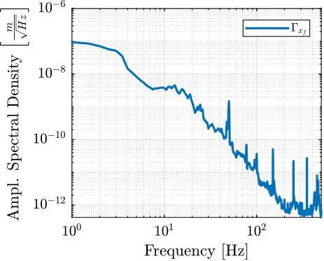
psd_xf = psd_V./abs(squeeze(freqresp(G_geo*g0, f, 'Hz'))).^2; % [m^2/Hz]The amplitude spectral density of the floor motion $\Gamma_{x_f}$ can be computed from the amplitude spectral density of measured voltage $\Gamma_{\hat{V}_{x_f}}$ using eqref:eq:uniaxial_asd_floor_motion. The estimated amplitude spectral density $\Gamma_{x_f}$ of the floor motion $x_f$ is shown in Figure ref:fig:uniaxial_asd_floor_motion_id31.
\begin{equation}\label{eq:uniaxial_asd_floor_motion} Γx_f(ω) = \frac{Γ_{\hat{V}x_f}(ω)}{|Ggeo(jω)| ⋅ g_0} \quad ≤ft[ m/\sqrt{\text{Hz}} \right]
\end{equation}
Stage Vibration
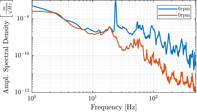
To estimate the vibrations induced by scanning the micro-station stages, two geophones are used, as shown in Figure ref:fig:uniaxial_ustation_dynamical_id_setup. The vertical relative velocity between the top platform of the micro hexapod and the granite is estimated in two cases: without moving the micro-station stages, and then during a Spindle rotation at 6rpm. The vibrations induced by the $T_y$ stage are not considered here because they have less amplitude than the vibrations induced by the $R_z$ stage and because the $T_y$ stage can be scanned at lower velocities if the induced vibrations are found to be an issue.
%% Estimation of the Spectral density of the stage vibrations

% Measured velocity of granite and hexapod during spindle rotation
% t: time in [s]
% vg: measured granite velocity [m/s]
% vg: measured micro-hexapod's top platform velocity [m/s]
load('meas_spindle_on.mat', 't', 'vg', 'vh');
spindle_off = load('meas_spindle_off.mat', 't', 'vg', 'vh'); % No Rotation

% Compute Power Spectral Density of the relative velocity between granite and hexapod during spindle rotation
Fs = 1/(t(2)-t(1)); % Sampling Frequency [Hz]
win = hanning(ceil(2*Fs)); % Hanning window

[psd_vft, f] = pwelch(vh-vg, win, [], [], Fs); % [(m/s)^2/Hz]
[psd_off, ~] = pwelch(spindle_off.vh-spindle_off.vg, win, [], [], Fs); % [(m/s)^2/Hz]

% Disable the Nano-Hexpod for now
model_config = struct();
model_config.nhexa = "none";
model_config.controller = "open_loop";

% Identify the transfer function from u to taum
clear io; io_i = 1;
io(io_i) = linio([mdl, '/micro_station/ft'], 1, 'openinput');  io_i = io_i + 1; % Stage Disturbance Force
io(io_i) = linio([mdl, '/micro_station/xg'], 1, 'openoutput'); io_i = io_i + 1; % Absolute motion of Granite
io(io_i) = linio([mdl, '/micro_station/xh'], 1, 'openoutput'); io_i = io_i + 1; % Absolute motion of Hexapod

% Perform the model extraction
G = linearize(mdl, io, 0.0);
G.InputName = {'ft'};
G.OutputName = {'Dg', 'Dh'};

% Power Spectral Density of the equivalent force ft [N/Hz^2]
psd_ft = (psd_vft./(2*pi*f).^2)./abs(squeeze(freqresp(G('Dh', 'ft') - G('Dg', 'ft'), f, 'Hz'))).^2;
The amplitude spectral density of the relative motion with and without the Spindle rotation are compared in Figure ref:fig:uniaxial_asd_vibration_spindle_rotation. It is shown that the spindle rotation increases the vibrations above $20\,\text{Hz}$. The sharp peak observed at $24\,\text{Hz}$ is believed to be induced by electromagnetic interference between the currents in the spindle motor phases and the geophone cable because this peak is not observed when rotating the spindle "by hand".
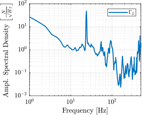
To compute the equivalent disturbance force $f_t$ (Figure ref:fig:uniaxial_model_micro_station) that induces such motion, the transfer function $G_{f_t}(s)$ from $f_t$ to the relative motion between the micro-hexapod's top platform and the granite $(x_{h} - x_{g})$ is extracted from the model. The amplitude spectral density $\Gamma_{f_{t}}$ of the disturbance force is them computed from eqref:eq:uniaxial_ft_asd and is shown in Figure ref:fig:uniaxial_asd_disturbance_force.
\begin{equation}\label{eq:uniaxial_ft_asd} Γ_{ft}(ω) = \frac{Γ_{Rz}(ω)}{|Gf_t(jω)|}
\end{equation}
Open-Loop Dynamic Noise Budgeting
<<sec:uniaxial_noise_budgeting>>
Introduction ignore
Now that a model of the acrshort:nass has been obtained (see section ref:sec:nano_station_model) and that the disturbances have been estimated (see section ref:sec:uniaxial_disturbances), it is possible to perform an open-loop dynamic noise budgeting.
To perform such noise budgeting, the disturbances need to be modeled by their spectral densities (done in section ref:sec:uniaxial_disturbances). Then, the transfer functions from disturbances to the performance metric (here the distance $d$) are computed (Section ref:ssec:uniaxial_noise_budget_sensitivity). Finally, these two types of information are combined to estimate the corresponding spectral density of the performance metric. This is very useful to identify what is limiting the performance of the system, or the compare the achievable performance with different system parameters (Section ref:ssec:uniaxial_noise_budget_result).
Sensitivity to disturbances
<<ssec:uniaxial_noise_budget_sensitivity>> From the uniaxial model of the acrshort:nass (Figure ref:fig:uniaxial_model_micro_station_nass), the transfer function from the disturbances ($f_s$, $x_f$ and $f_t$) to the displacement $d$ are computed.
This is done for two extreme sample masses $m_s = 1\,\text{kg}$ and $m_s = 50\,\text{kg}$ and three nano-hexapod stiffnesses:
- $k_n = 0.01\,N/\mu m$ that represents a voice coil actuator with soft flexible guiding
- $k_n = 1\,N/\mu m$ that represents a voice coil actuator with a stiff flexible guiding or a mechanically amplified piezoelectric actuator
- $k_n = 100\,N/\mu m$ that represents a stiff piezoelectric stack actuator
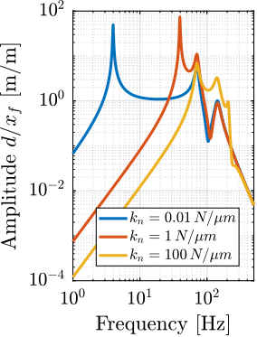
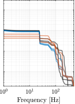
The obtained sensitivity to disturbances for the three nano-hexapod stiffnesses are shown in Figure ref:fig:uniaxial_sensitivity_disturbances_nano_hexapod_stiffnesses for the sample mass $m_s = 1\,\text{kg}$ (the same conclusions can be drawn with $m_s = 50\,\text{kg}$):
- The soft nano-hexapod is more sensitive to forces applied on the sample (cable forces for instance), which is expected due to its lower stiffness (Figure ref:fig:uniaxial_sensitivity_disturbances_nano_hexapod_stiffnesses_fs)
- Between the suspension mode of the nano-hexapod (here at 5Hz for the soft nano-hexapod) and the first mode of the micro-station (here at 70Hz), the disturbances induced by the stage vibrations are filtered out (Figure ref:fig:uniaxial_sensitivity_disturbances_nano_hexapod_stiffnesses_ft)
- Above the suspension mode of the nano-hexapod, the sample's inertial motion is unaffected by the floor motion; therefore, the sensitivity to floor motion is close to $1$ (Figure ref:fig:uniaxial_sensitivity_disturbances_nano_hexapod_stiffnesses_xf)
Open-Loop Dynamic Noise Budgeting
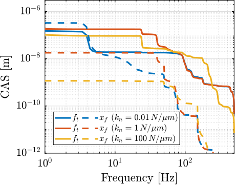
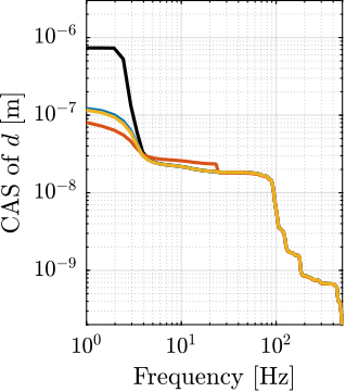
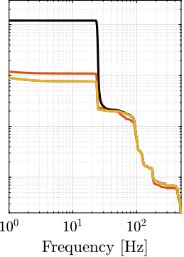
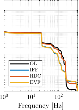
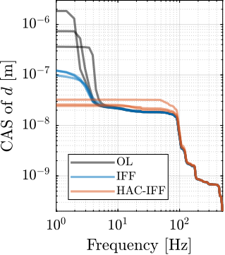
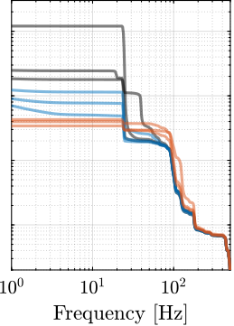
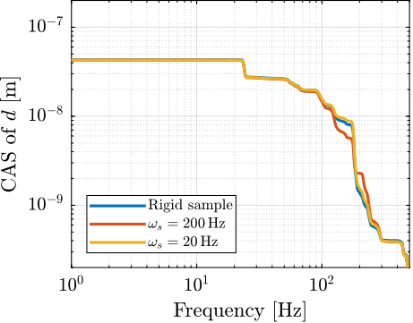
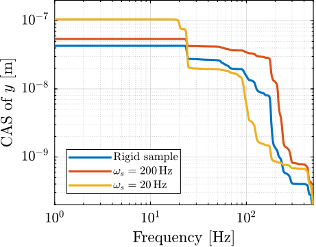
<<ssec:uniaxial_noise_budget_result>> Now, the amplitude spectral densities of the disturbances are considered to estimate the residual motion $d$ for each nano-hexapod and sample configuration. The Cumulative Amplitude Spectrum of the relative motion $d$ due to both floor motion $x_f$ and stage vibrations $f_t$ are shown in Figure ref:fig:uniaxial_cas_d_disturbances_stiffnesses for the three nano-hexapod stiffnesses. It is shown that the effect of floor motion is much less than that of stage vibrations, except for the soft nano-hexapod below $5\,\text{Hz}$.
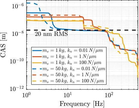
The total cumulative amplitude spectrum of $d$ for the three nano-hexapod stiffnesses and for the two samples masses are shown in Figure ref:fig:uniaxial_cas_d_disturbances_payload_masses. The conclusion is that the sample mass has little effect on the cumulative amplitude spectrum of the relative motion $d$.
Conclusion
The open-loop residual vibrations of $d$ can be estimated from the low-frequency value of the cumulative amplitude spectrum in Figure ref:fig:uniaxial_cas_d_disturbances_payload_masses. This residual vibration of $d$ is found to be in the order of $100\,nm\,\text{RMS}$ for the stiff nano-hexapod ($k_n = 100\,N/\mu m$), $200\,nm\,\text{RMS}$ for the relatively stiff nano-hexapod ($k_n = 1\,N/\mu m$) and $1\,\mu m\,\text{RMS}$ for the soft nano-hexapod ($k_n = 0.01\,N/\mu m$). From this analysis, it may be concluded that the stiffer the nano-hexapod the better.
However, what is more important is the closed-loop residual vibration of $d$ (i.e., while the feedback controller is used). The goal is to obtain a closed-loop residual vibration $\epsilon_d \approx 20\,nm\,\text{RMS}$ (represented by an horizontal dashed black line in Figure ref:fig:uniaxial_cas_d_disturbances_payload_masses). The bandwidth of the feedback controller leading to a closed-loop residual vibration of $20\,nm\,\text{RMS}$ can be estimated as the frequency at which the cumulative amplitude spectrum crosses the black dashed line in Figure ref:fig:uniaxial_cas_d_disturbances_payload_masses.
A closed loop bandwidth of $\approx 10\,\text{Hz}$ is found for the soft nano-hexapod ($k_n = 0.01\,N/\mu m$), $\approx 50\,\text{Hz}$ for the relatively stiff nano-hexapod ($k_n = 1\,N/\mu m$), and $\approx 100\,\text{Hz}$ for the stiff nano-hexapod ($k_n = 100\,N/\mu m$). Therefore, while the open-loop vibration is the lowest for the stiff nano-hexapod, it requires the largest feedback bandwidth to meet the specifications.
The advantage of the soft nano-hexapod can be explained by its natural isolation from the micro-station vibration above its suspension mode, as shown in Figure ref:fig:uniaxial_sensitivity_disturbances_nano_hexapod_stiffnesses_ft.
Active Damping
<<sec:uniaxial_active_damping>>
Introduction ignore
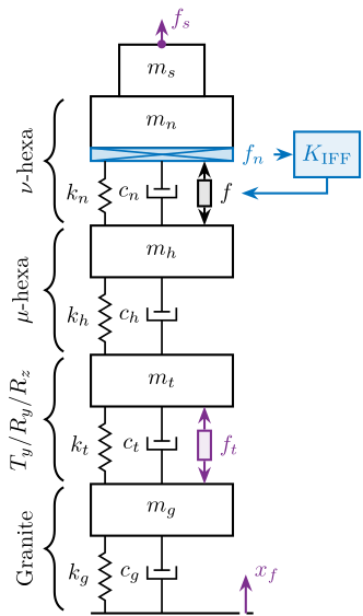
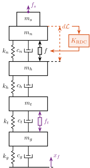
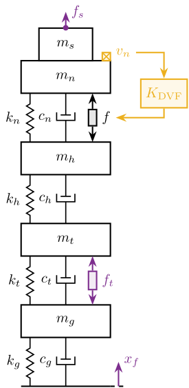
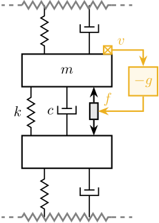
In this section, three active damping techniques are applied to the nano-hexapod (see Figure ref:fig:uniaxial_active_damping_strategies): Integral Force Feedback (IFF) cite:preumont91_activ, Relative Damping Control (RDC) cite:&preumont18_vibrat_contr_activ_struc_fourt_edition Chapter 7.2 and Direct Velocity Feedback (DVF) cite:karnopp74_vibrat_contr_using_semi_activ_force_gener,serrand00_multic_feedb_contr_isolat_base_excit_vibrat,preumont02_force_feedb_versus_accel_feedb.
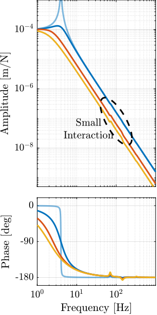
These damping strategies are first described (Section ref:ssec:uniaxial_active_damping_strategies) and are then compared in terms of achievable damping of the nano-hexapod mode (Section ref:ssec:uniaxial_active_damping_achievable_damping), reduction of the effect of disturbances (i.e., $x_f$, $f_t$ and $f_s$) on the displacement $d$ (Sections ref:ssec:uniaxial_active_damping_sensitivity_disturbances).
\begin{tikzpicture}
  % ====================
  % Parameters
  % ====================
  \def\massw{2.2}  % Width of the masses
  \def\massh{0.8}  % Height of the masses
  \def\spaceh{1.2} % Height of the springs/dampers
  \def\dispw{0.4}  % Width of the dashed line for the displacement
  \def\disph{0.3}  % Height of the arrow for the displacements
  \def\bracs{0.05} % Brace spacing vertically
  \def\brach{-12pt} % Brace shift horizontaly
  \def\fsensh{0.2} % Height of the force sensor
  \def\velsize{0.2} % Size of the velocity sensor
  % ====================

  % IFF
  \begin{scope}
    % ====================
    % Ground
    % ====================
    \draw (-0.5*\massw, 0) -- (0.5*\massw, 0);
    \draw[dashed] (0.5*\massw, 0) -- ++(\dispw, 0);
    \draw[->, color=colorpurple] (0.5*\massw+0.5*\dispw, 0) -- ++(0, 2*\disph) node[right, color=colorpurple]{$x_{f}$};
    % ====================

    % ====================
    % Granite
    \begin{scope}[shift={(0, 0)}]
      % Mass
      \draw[fill=white] (-0.5*\massw, \spaceh) rectangle (0.5*\massw, \spaceh+\massh) node[pos=0.5]{$m_{g}$};

      % Spring, Damper, and Actuator
      \draw[spring] (-0.4*\massw, 0) -- (-0.4*\massw, \spaceh) node[midway, left=0.1]{$k_{g}$};
      \draw[damper] (0, 0)           -- ( 0, \spaceh)          node[midway, left=0.2]{$c_{g}$};

      % Legend
      \draw[decorate, decoration={brace, amplitude=8pt}, xshift=\brach] %
      (-0.5*\massw, \bracs) -- (-0.5*\massw, \spaceh+\massh-\bracs) node[midway,rotate=90,anchor=south,yshift=10pt]{Granite};
    \end{scope}
    % ====================


    % ====================
    % Stages
    \begin{scope}[shift={(0, \spaceh+\massh)}]
      % Mass
      \draw[fill=white] (-0.5*\massw, \spaceh) rectangle (0.5*\massw, \spaceh+\massh) node[pos=0.5]{$m_{t}$};

      % Spring, Damper, and Actuator
      \draw[spring] (-0.4*\massw, 0) -- (-0.4*\massw, \spaceh) node[midway, left=0.1]{$k_{t}$};
      \draw[damper] (0, 0)           -- ( 0, \spaceh)          node[midway, left=0.2]{$c_{t}$};
      \draw[actuator={0.45}{0.2}{colorpurple}] ( 0.3*\massw, 0) -- (0.3*\massw, \spaceh) node[midway, right=0.1, color=colorpurple](ft){$f_{t}$};

      % Legend
      \draw[decorate, decoration={brace, amplitude=8pt}, xshift=\brach] %
      (-0.5*\massw, \bracs) -- (-0.5*\massw, \spaceh+\massh-\bracs) node[midway,rotate=90,anchor=south,yshift=10pt]{$T_y$/$R_y$/$R_z$};
    \end{scope}
    % ====================


    % ====================
    % Hexapod
    \begin{scope}[shift={(0, 2*(\spaceh+\massh))}]
      % Mass
      \draw[fill=white] (-0.5*\massw, \spaceh) rectangle (0.5*\massw, \spaceh+\massh) node[pos=0.5]{$m_h$};

      % Spring, Damper, and Actuator
      \draw[spring] (-0.4*\massw, 0) -- (-0.4*\massw, \spaceh) node[midway, left=0.1]{$k_h$};
      \draw[damper] (0, 0)           -- ( 0, \spaceh)          node[midway, left=0.2]{$c_h$};

      % Legend
      \draw[decorate, decoration={brace, amplitude=8pt}, xshift=\brach] %
      (-0.5*\massw, \bracs) -- (-0.5*\massw, \spaceh+\massh-\bracs) node[midway,rotate=90,anchor=south,yshift=10pt]{$\mu\text{-hexa}$};
    \end{scope}
    % ====================


    % ====================
    % NASS
    \begin{scope}[shift={(0, 3*(\spaceh+\massh))}]
      % Mass
      \draw[fill=white] (-0.5*\massw, \spaceh) rectangle (0.5*\massw, \spaceh+\massh) node[pos=0.5]{$m_{n}$};

      % Force Sensor
      \node[forcesensor={\massw}{\fsensh}{colorblue}] (fsensn) at (0, \spaceh-\fsensh){};
      \node[right, color=colorblue] (fn) at (fsensn.east) {$f_n$};

      % Spring, Damper, and Actuator
      \draw[spring] (-0.4*\massw, 0) -- (-0.4*\massw, \spaceh-\fsensh) node[midway, left=0.1]{$k_{n}$};
      \draw[damper] (0, 0)           -- ( 0, \spaceh-\fsensh)          node[midway, left=0.2]{$c_{n}$};
      \draw[actuator={0.4}{0.2}{black}] ( 0.3*\massw, 0) -- (	0.3*\massw, \spaceh-\fsensh) node[midway, right=0.1](f){$f$};

      % Legend
      \draw[decorate, decoration={brace, amplitude=8pt}, xshift=\brach] %
      (-0.5*\massw, \bracs) -- (-0.5*\massw, \spaceh+\massh-\bracs) node[midway,rotate=90,anchor=south,yshift=10pt]{$\nu\text{-hexa}$};
    \end{scope}
    % ====================

    % ====================
    % sample
    \begin{scope}[shift={(0, 4*(\spaceh+\massh))}]
      % Mass
      \draw[fill=white] (-0.3*\massw, 0) rectangle (0.3*\massw, \massh) node[pos=0.5]{$m_{s}$};

      % External Force
      \draw[->, color=colorpurple] (0, \massh) node[]{$\bullet$} -- ++(0, 0.5*\massh) node[right, color=colorpurple]{$f_s$};
    \end{scope}
    % ====================

    % ====================
    % IFF Control
    \node[block={2em}{2em}, right=0.3 of fn, color=colorblue, fill=colorblue!10!white] (iff) {$K_{\text{IFF}}$};
    \draw[->, draw=colorblue] (fn.east) -- (iff.west);
    \draw[->, draw=colorblue] (iff.south) |- (f.east);
    % ====================
  \end{scope}
\end{tikzpicture}\begin{tikzpicture}
% ====================
% Parameters
% ====================
\def\massw{2.2} % Width of the masses
\def\massh{0.8} % Height of the masses
\def\spaceh{1.2} % Height of the springs/dampers
\def\dispw{0.4} % Width of the dashed line for the displacement
\def\disph{0.3} % Height of the arrow for the displacements
\def\bracs{0.05} % Brace spacing vertically
\def\brach{-12pt} % Brace shift horizontaly
\def\fsensh{0.2} % Height of the force sensor
\def\velsize{0.2} % Size of the velocity sensor
% ====================
% RDC
\begin{scope}
% ====================
% Ground
% ====================
\draw (-0.5*\massw, 0) -- (0.5*\massw, 0);
\draw[dashed] (0.5*\massw, 0) -- ++(\dispw, 0);
\draw[->, color=colorpurple] (0.5*\massw+0.5*\dispw, 0) -- ++(0, 2*\disph) node[right, color=colorpurple]{$x_{f}$};
% ====================
% ====================
% Granite
\begin{scope}[shift={(0, 0)}]
% Mass
\draw[fill=white] (-0.5*\massw, \spaceh) rectangle (0.5*\massw, \spaceh+\massh) node[pos=0.5]{$m_{g}$};
% Spring, Damper, and Actuator
\draw[spring] (-0.4*\massw, 0) -- (-0.4*\massw, \spaceh) node[midway, left=0.1]{$k_{g}$};
\draw[damper] (0, 0) -- ( 0, \spaceh) node[midway, left=0.2]{$c_{g}$};
\end{scope}
% ====================
% ====================
% Stages
\begin{scope}[shift={(0, \spaceh+\massh)}]
% Mass
\draw[fill=white] (-0.5*\massw, \spaceh) rectangle (0.5*\massw, \spaceh+\massh) node[pos=0.5]{$m_{t}$};
% Spring, Damper, and Actuator
\draw[spring] (-0.4*\massw, 0) -- (-0.4*\massw, \spaceh) node[midway, left=0.1]{$k_{t}$};
\draw[damper] (0, 0) -- ( 0, \spaceh) node[midway, left=0.2]{$c_{t}$};
\draw[actuator={0.45}{0.2}{colorpurple}] ( 0.3*\massw, 0) -- (0.3*\massw, \spaceh) node[midway, right=0.1, color=colorpurple](ft){$f_{t}$};
\end{scope}
% ====================
% ====================
% Hexapod
\begin{scope}[shift={(0, 2*(\spaceh+\massh))}]
% Mass
\draw[fill=white] (-0.5*\massw, \spaceh) rectangle (0.5*\massw, \spaceh+\massh) node[pos=0.5]{$m_h$};
% Spring, Damper, and Actuator
\draw[spring] (-0.4*\massw, 0) -- (-0.4*\massw, \spaceh) node[midway, left=0.1]{$k_h$};
\draw[damper] (0, 0) -- ( 0, \spaceh) node[midway, left=0.2]{$c_h$};
\draw[dashed] (0.5*\massw, \spaceh+\massh) -- ++(2*\dispw, 0) coordinate(drbot);
\end{scope}
% ====================
% ====================
% NASS
\begin{scope}[shift={(0, 3*(\spaceh+\massh))}]
% Mass
\draw[fill=white] (-0.5*\massw, \spaceh) rectangle (0.5*\massw, \spaceh+\massh) node[pos=0.5]{$m_{n}$};
% Spring, Damper, and Actuator
\draw[spring] (-0.4*\massw, 0) -- (-0.4*\massw, \spaceh) node[midway, left=0.1]{$k_{n}$};
\draw[damper] (0, 0) -- ( 0, \spaceh) node[midway, left=0.2]{$c_{n}$};
\draw[actuator={0.4}{0.2}{black}] ( 0.3*\massw, 0) -- (0.3*\massw, \spaceh) node[midway, right=0.1](f){$f$};
\draw[dashed, draw=colorred] (0.5*\massw, \spaceh+\massh) -- ++(2*\dispw, 0) coordinate(drtop);
\end{scope}
% ====================
% ====================
% sample
\begin{scope}[shift={(0, 4*(\spaceh+\massh))}]
% Mass
\draw[fill=white] (-0.3*\massw, 0) rectangle (0.3*\massw, \massh) node[pos=0.5]{$m_{s}$};
% External Force
\draw[->, color=colorpurple] (0, \massh) node[]{$\bullet$} -- ++(0, 0.5*\massh) node[right, color=colorpurple]{$f_s$};
\end{scope}
% ====================
\draw[<->, dashed, draw=colorred] ($(drbot)+(-0.1, 0)$) -- ($(drtop)+(-0.1, 0)$) node[right, color=colorred](dr){$d\mathcal{L}$};
% ====================
% RDC Control
\node[block={2em}{2em}, below right=0.2 and -0.2 of dr, color=colorred, fill=colorred!10!white] (rdc) {$K_{\text{RDC}}$};
\draw[->, draw=colorred] (dr.east) -| (rdc.north);
\draw[->, draw=colorred] (rdc.south) |- (f.east);
% ====================
\end{scope}
\end{tikzpicture}\begin{tikzpicture}
% ====================
% Parameters
% ====================
\def\massw{2.2} % Width of the masses
\def\massh{0.8} % Height of the masses
\def\spaceh{1.2} % Height of the springs/dampers
\def\dispw{0.4} % Width of the dashed line for the displacement
\def\disph{0.3} % Height of the arrow for the displacements
\def\bracs{0.05} % Brace spacing vertically
\def\brach{-12pt} % Brace shift horizontaly
\def\fsensh{0.2} % Height of the force sensor
\def\velsize{0.2} % Size of the velocity sensor
% ====================
% DVF
\begin{scope}
% ====================
% Ground
% ====================
\draw (-0.5*\massw, 0) -- (0.5*\massw, 0);
\draw[dashed] (0.5*\massw, 0) -- ++(\dispw, 0);
\draw[->, color=colorpurple] (0.5*\massw+0.5*\dispw, 0) -- ++(0, 2*\disph) node[right, color=colorpurple]{$x_{f}$};
% ====================
% ====================
% Marble
\begin{scope}[shift={(0, 0)}]
% Mass
\draw[fill=white] (-0.5*\massw, \spaceh) rectangle (0.5*\massw, \spaceh+\massh) node[pos=0.5]{$m_{g}$};
% Spring, Damper, and Actuator
\draw[spring] (-0.4*\massw, 0) -- (-0.4*\massw, \spaceh) node[midway, left=0.1]{$k_{g}$};
\draw[damper] (0, 0) -- ( 0, \spaceh) node[midway, left=0.2]{$c_{g}$};
\end{scope}
% ====================
% ====================
% Stages
\begin{scope}[shift={(0, \spaceh+\massh)}]
% Mass
\draw[fill=white] (-0.5*\massw, \spaceh) rectangle (0.5*\massw, \spaceh+\massh) node[pos=0.5]{$m_{t}$};
% Spring, Damper, and Actuator
\draw[spring] (-0.4*\massw, 0) -- (-0.4*\massw, \spaceh) node[midway, left=0.1]{$k_{t}$};
\draw[damper] (0, 0) -- ( 0, \spaceh) node[midway, left=0.2]{$c_{t}$};
\draw[actuator={0.45}{0.2}{colorpurple}] ( 0.3*\massw, 0) -- (0.3*\massw, \spaceh) node[midway, right=0.1, color=colorpurple](ft){$f_{t}$};
\end{scope}
% ====================
% ====================
% Hexapod
\begin{scope}[shift={(0, 2*(\spaceh+\massh))}]
% Mass
\draw[fill=white] (-0.5*\massw, \spaceh) rectangle (0.5*\massw, \spaceh+\massh) node[pos=0.5]{$m_{h}$};
% Spring, Damper, and Actuator
\draw[spring] (-0.4*\massw, 0) -- (-0.4*\massw, \spaceh) node[midway, left=0.1]{$k_{h}$};
\draw[damper] (0, 0) -- ( 0, \spaceh) node[midway, left=0.2]{$c_{h}$};
\end{scope}
% ====================
% ====================
% NASS
\begin{scope}[shift={(0, 3*(\spaceh+\massh))}]
% Mass
\draw[fill=white] (-0.5*\massw, \spaceh) rectangle (0.5*\massw, \spaceh+\massh) node[pos=0.5]{$m_{n}$};
% Spring, Damper, and Actuator
\draw[spring] (-0.4*\massw, 0) -- (-0.4*\massw, \spaceh) node[midway, left=0.1]{$k_{n}$};
\draw[damper] (0, 0) -- ( 0, \spaceh) node[midway, left=0.2]{$c_{n}$};
\draw[actuator={0.4}{0.2}{black}] ( 0.3*\massw, 0) -- (0.3*\massw, \spaceh) node[midway, right=0.1](f){$f$};
% Velocity Sensor
\node[inertialsensor={\velsize}{coloryellow}] (veln) at (0.5*\massw, \spaceh+\massh) {};
\node[right, color=coloryellow] (xn) at (veln.north east) {$v_n$};
\end{scope}
% ====================
% ====================
% sample
\begin{scope}[shift={(0, 4*(\spaceh+\massh))}]
% Mass
\draw[fill=white] (-0.3*\massw, 0) rectangle (0.3*\massw, \massh) node[pos=0.5]{$m_{s}$};
% External Force
\draw[->, color=colorpurple] (0, \massh) node[]{$\bullet$} -- ++(0, 0.5*\massh) node[right, color=colorpurple]{$f_s$};
\end{scope}
% ====================
% ====================
% DVF Control
\node[block={2em}{2em}, below right=0.4 and 0.1 of xn, color=coloryellow, fill=coloryellow!10!white] (ppf) {$K_{\text{DVF}}$};
\draw[->, draw=coloryellow] (xn.east) -| (ppf.north);
\draw[->, draw=coloryellow] (ppf.south) |- (f.east);
% ====================
\end{scope}
\end{tikzpicture}Active Damping Strategies
<<ssec:uniaxial_active_damping_strategies>>
Integral Force Feedback (IFF)
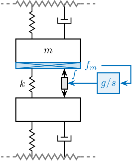
The Integral Force Feedback strategy consists of using a force sensor in series with the actuator (see Figure ref:fig:uniaxial_active_damping_iff_schematic) and applying an "integral" feedback controller eqref:eq:uniaxial_iff_controller.
\begin{equation}\label{eq:uniaxial_iff_controller} \boxed{K_{\text{IFF}}(s) = \frac{g}{s}}
\end{equation}
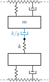
The mechanical equivalent of this IFF strategy is a dashpot in series with the actuator stiffness with a damping coefficient equal to the stiffness of the actuator divided by the controller gain $k/g$ (see Figure ref:fig:uniaxial_active_damping_iff_equiv).
\begin{tikzpicture}
  % ====================
  % Parameters
  % ====================
  \def\massw{2.2}  % Width of the masses
  \def\massh{0.8}  % Height of the masses
  \def\spaceh{1.2} % Height of the springs/dampers
  \def\dispw{0.4}  % Width of the dashed line for the displacement
  \def\disph{0.3}  % Height of the arrow for the displacements
  \def\bracs{0.05} % Brace spacing vertically
  \def\brach{-12pt} % Brace shift horizontaly
  \def\fsensh{0.2} % Height of the force sensor
  \def\velsize{0.2} % Size of the velocity sensor
  % ====================

  \begin{scope}
    % ====================
    % Stage Below
    \begin{scope}
      \draw[fill=white] (-0.5*\massw, \spaceh) rectangle (0.5*\massw, \spaceh+\massh);
      \draw[spring] (-0.25*\massw, 0) -- (-0.25*\massw, \spaceh);
      \draw[damper] ( 0.25*\massw, 0) -- ( 0.25*\massw, \spaceh);
      \draw[decorate,decoration={zigzag,segment length=6pt},draw=black!50!white,very thick] (-0.5*\massw, 0) -- (0.5*\massw, 0);
      \draw[draw=black!50!white,very thick, dashed] (-0.5*\massw, 0) -- ++(-0.5, 0);
      \draw[draw=black!50!white,very thick, dashed] ( 0.5*\massw, 0) -- ++( 0.5, 0);
    \end{scope}
    % ====================

    % ====================
    % NASS
    \begin{scope}[shift={(0, \spaceh+\massh)}]
      \draw[fill=white] (-0.5*\massw, \spaceh) rectangle (0.5*\massw, \spaceh+\massh) node[pos=0.5]{$m$};
      \node[forcesensor={\massw}{\fsensh}{colorblue}] (fsensn) at (0, \spaceh-\fsensh){};
      \node[right, color=colorblue] (fn) at (fsensn.east) {$f_m$};
      \draw[spring] (-0.25*\massw, 0) -- (-0.25*\massw, \spaceh-\fsensh) node[midway, left=0.1]{$k$};
      \draw[actuator={0.4}{0.2}{black}] ( 0.25*\massw, 0) -- (0.25*\massw, \spaceh-\fsensh) coordinate[midway, shift={(0.1,0)}](f);
    \end{scope}
    % ====================

    % ====================
    % Stage Above
    \begin{scope}[shift={(0, 2*(\spaceh+\massh))}]
      \draw[spring] (-0.25*\massw, 0) -- (-0.25*\massw, \spaceh);
      \draw[damper] ( 0.25*\massw, 0) -- ( 0.25*\massw, \spaceh);
      \draw[decorate,decoration={zigzag,segment length=6pt},draw=black!50!white,very thick] (-0.5*\massw, \spaceh) -- (0.5*\massw, \spaceh);
      \draw[draw=black!50!white,very thick, dashed] (-0.5*\massw, \spaceh) -- ++(-0.5, 0);
      \draw[draw=black!50!white,very thick, dashed] ( 0.5*\massw, \spaceh) -- ++( 0.5, 0);
    \end{scope}
    % ====================

    % ====================
    % IFF Control
    \node[block={2em}{2em}, right=1.0 of f, color=colorblue, fill=colorblue!10!white] (iff) {$g/s$};
    \draw[->, draw=colorblue] (fn.east) -- ++(1.0, 0) |- (iff.east);
    \draw[->, draw=colorblue] (iff.west) -- (f.east) node[above right, color=colorblue]{$f$};
    % ====================
  \end{scope}
\end{tikzpicture}\begin{tikzpicture}
% ====================
% Parameters
% ====================
\def\massw{2.2} % Width of the masses
\def\massh{0.8} % Height of the masses
\def\spaceh{1.2} % Height of the springs/dampers
\def\dispw{0.4} % Width of the dashed line for the displacement
\def\disph{0.3} % Height of the arrow for the displacements
\def\bracs{0.05} % Brace spacing vertically
\def\brach{-12pt} % Brace shift horizontaly
\def\fsensh{0.2} % Height of the force sensor
\def\velsize{0.2} % Size of the velocity sensor
% ====================
\begin{scope}[shift={(6, 0)}]
% ====================
% Stage Below
\begin{scope}
\draw[fill=white] (-0.5*\massw, 0.8*\spaceh) rectangle (0.5*\massw, 0.8*\spaceh+\massh);
\draw[spring] (-0.25*\massw, 0) -- (-0.25*\massw, 0.8*\spaceh);
\draw[damper] ( 0.25*\massw, 0) -- ( 0.25*\massw, 0.8*\spaceh);
\draw[decorate,decoration={zigzag,segment length=6pt},draw=black!50!white,very thick] (-0.5*\massw, 0) -- (0.5*\massw, 0);
\draw[draw=black!50!white,very thick, dashed] (-0.5*\massw, 0) -- ++(-0.5, 0);
\draw[draw=black!50!white,very thick, dashed] ( 0.5*\massw, 0) -- ++( 0.5, 0);
\end{scope}
% ====================
% ====================
% NASS
\begin{scope}[shift={(0, 0.8*\spaceh+\massh)}]
\draw[fill=white] (-0.5*\massw, 1.4*\spaceh) rectangle (0.5*\massw, 1.4*\spaceh+\massh) node[pos=0.5]{$m$};
\draw[spring] (0, 0) -- node[midway, left=0.1]{$k$} (0, 0.8*\spaceh);
\draw[damper={colorblue}{}{}] (0, 0.8*\spaceh) node[branch]{} -- (0, 1.4*\spaceh) node[midway, left=0.2, color=colorblue]{$k/g$};
\end{scope}
% ====================
% ====================
% Stage Above
\begin{scope}[shift={(0, 0.8*\spaceh+\massh+1.4*\spaceh+\massh)}]
\draw[spring] (-0.25*\massw, 0) -- (-0.25*\massw, 0.8*\spaceh);
\draw[damper] ( 0.25*\massw, 0) -- ( 0.25*\massw, 0.8*\spaceh);
\draw[decorate,decoration={zigzag,segment length=6pt},draw=black!50!white,very thick] (-0.5*\massw, 0.8*\spaceh) -- (0.5*\massw, 0.8*\spaceh);
\draw[draw=black!50!white,very thick, dashed] (-0.5*\massw, 0.8*\spaceh) -- ++(-0.5, 0);
\draw[draw=black!50!white,very thick, dashed] ( 0.5*\massw, 0.8*\spaceh) -- ++( 0.5, 0);
\end{scope}
% ====================
\end{scope}
% % Equiv
% \draw[double, <->, draw=colorblue, double distance=1.5] (3.0, 1.5*\spaceh+\massh) -- ++(1.5,0);
\end{tikzpicture}Relative Damping Control (RDC)
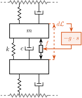
For the Relative Damping Control strategy, a relative motion sensor that measures the motion of the actuator is used (see Figure ref:fig:uniaxial_active_damping_rdc_schematic) and a "derivative" feedback controller is used eqref:eq:uniaxial_rdc_controller.
\begin{equation}\label{eq:uniaxial_rdc_controller} \boxed{K_{\text{RDC}}(s) = - g ⋅ s}
\end{equation}
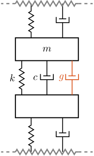
The mechanical equivalent of acrshort:rdc is a dashpot in parallel with the actuator with a damping coefficient equal to the controller gain $g$ (see Figure ref:fig:uniaxial_active_damping_rdc_equiv).
\begin{tikzpicture}
  % ====================
  % Parameters
  % ====================
  \def\massw{2.2}  % Width of the masses
  \def\massh{0.8}  % Height of the masses
  \def\spaceh{1.2} % Height of the springs/dampers
  \def\dispw{0.4}  % Width of the dashed line for the displacement
  \def\disph{0.3}  % Height of the arrow for the displacements
  \def\bracs{0.05} % Brace spacing vertically
  \def\brach{-12pt} % Brace shift horizontaly
  \def\fsensh{0.2} % Height of the force sensor
  \def\velsize{0.2} % Size of the velocity sensor
  % ====================

  \begin{scope}
    % ====================
    % Stage Below
    \begin{scope}
      \draw[fill=white] (-0.5*\massw, \spaceh) rectangle (0.5*\massw, \spaceh+\massh);
      \draw[spring] (-0.25*\massw, 0) -- (-0.25*\massw, \spaceh);
      \draw[damper] ( 0.25*\massw, 0) -- ( 0.25*\massw, \spaceh);

      \draw[dashed, draw=colorred] (0.5*\massw, \spaceh+\massh) -- ++(1*\dispw, 0) coordinate(drbot);
      \draw[decorate,decoration={zigzag,segment length=6pt},draw=black!50!white,very thick] (-0.5*\massw, 0) -- (0.5*\massw, 0);
      \draw[draw=black!50!white,very thick, dashed] (-0.5*\massw, 0) -- ++(-0.5, 0);
      \draw[draw=black!50!white,very thick, dashed] ( 0.5*\massw, 0) -- ++( 0.5, 0);
    \end{scope}
    % ====================

    % ====================
    % NASS
    \begin{scope}[shift={(0, \spaceh+\massh)}]
      \draw[fill=white] (-0.5*\massw, \spaceh) rectangle (0.5*\massw, \spaceh+\massh) node[pos=0.5]{$m$};
      \draw[spring] (-0.4*\massw, 0) -- (-0.4*\massw, \spaceh) node[midway, left=0.1]{$k$};
      \draw[damper] (0, 0)           -- ( 0, \spaceh)          node[midway, left=0.2]{$c$};
      \draw[actuator={0.4}{0.2}{black}] ( 0.3*\massw, 0) -- (0.3*\massw, \spaceh) coordinate[midway, shift={(0.1,0)}](f);

      \draw[dashed, draw=colorred] (0.5*\massw, \spaceh+\massh) -- ++(1*\dispw, 0) coordinate(drtop);
    \end{scope}
    % ====================

    % ====================
    % Stage Above
    \begin{scope}[shift={(0, 2*(\spaceh+\massh))}]
      \draw[spring] (-0.25*\massw, 0) -- (-0.25*\massw, \spaceh);
      \draw[damper] ( 0.25*\massw, 0) -- ( 0.25*\massw, \spaceh);

      \draw[decorate,decoration={zigzag,segment length=6pt},draw=black!50!white,very thick] (-0.5*\massw, \spaceh) -- (0.5*\massw, \spaceh);
      \draw[draw=black!50!white,very thick, dashed] (-0.5*\massw, \spaceh) -- ++(-0.5, 0);
      \draw[draw=black!50!white,very thick, dashed] ( 0.5*\massw, \spaceh) -- ++( 0.5, 0);
    \end{scope}
    % ====================

    \draw[<->, dashed, draw=colorred] ($(drbot)+(-0.1, 0)$) -- ($(drtop)+(-0.1, 0)$) node[right, color=colorred](dr){$d\mathcal{L}$};
    % ====================
    % RDC Control
    \node[block={2em}{2em}, below right=0.2 and -0.3 of dr, color=colorred, fill=colorred!10!white] (rdc) {$-g \cdot s$};
    \draw[->, draw=colorred] (dr.east) -| (rdc.north);
    \draw[->, draw=colorred] (rdc.south) |- (f.east) node[above right, color=colorred]{$f$};
    % ====================
  \end{scope}
\end{tikzpicture}\begin{tikzpicture}
% ====================
% Parameters
% ====================
\def\massw{2.2} % Width of the masses
\def\massh{0.8} % Height of the masses
\def\spaceh{1.2} % Height of the springs/dampers
\def\dispw{0.4} % Width of the dashed line for the displacement
\def\disph{0.3} % Height of the arrow for the displacements
\def\bracs{0.05} % Brace spacing vertically
\def\brach{-12pt} % Brace shift horizontaly
\def\fsensh{0.2} % Height of the force sensor
\def\velsize{0.2} % Size of the velocity sensor
% ====================
\begin{scope}
% ====================
% Stage Below
\begin{scope}
\draw[fill=white] (-0.5*\massw, \spaceh) rectangle (0.5*\massw, \spaceh+\massh);
\draw[spring] (-0.25*\massw, 0) -- (-0.25*\massw, \spaceh);
\draw[damper] ( 0.25*\massw, 0) -- ( 0.25*\massw, \spaceh);
\draw[decorate,decoration={zigzag,segment length=6pt},draw=black!50!white,very thick] (-0.5*\massw, 0) -- (0.5*\massw, 0);
\draw[draw=black!50!white,very thick, dashed] (-0.5*\massw, 0) -- ++(-0.5, 0);
\draw[draw=black!50!white,very thick, dashed] ( 0.5*\massw, 0) -- ++( 0.5, 0);
\end{scope}
% ====================
% ====================
% NASS
\begin{scope}[shift={(0, \spaceh+\massh)}]
\draw[fill=white] (-0.5*\massw, \spaceh) rectangle (0.5*\massw, \spaceh+\massh) node[pos=0.5]{$m$};
\draw[spring] (-0.4*\massw, 0) -- (-0.4*\massw, \spaceh) node[midway, left=0.1]{$k$};
\draw[damper] (0, 0) -- ( 0, \spaceh) node[midway, left=0.2]{$c$};
\draw[damper={colorred}{}{}] ( 0.4*\massw, 0) -- ( 0.4*\massw, \spaceh) node[midway, left=0.15, color=colorred]{$g$};
\end{scope}
% ====================
% ====================
% Stage Above
\begin{scope}[shift={(0, 2*(\spaceh+\massh))}]
\draw[spring] (-0.25*\massw, 0) -- (-0.25*\massw, \spaceh);
\draw[damper] ( 0.25*\massw, 0) -- ( 0.25*\massw, \spaceh);
\draw[decorate,decoration={zigzag,segment length=6pt},draw=black!50!white,very thick] (-0.5*\massw, \spaceh) -- (0.5*\massw, \spaceh);
\draw[draw=black!50!white,very thick, dashed] (-0.5*\massw, \spaceh) -- ++(-0.5, 0);
\draw[draw=black!50!white,very thick, dashed] ( 0.5*\massw, \spaceh) -- ++( 0.5, 0);
\end{scope}
% ====================
\end{scope}
% % Equiv
% \draw[double, <->, draw=colorred, double distance=1.5] (3.0, 1.5*\spaceh+\massh) -- ++(1.5,0);
\end{tikzpicture}Direct Velocity Feedback (DVF)
Finally, the direct velocity feedback strategy consists of using an inertial sensor (usually a geophone) that measures the "absolute" velocity of the body fixed on top of the actuator (see Figure ref:fig:uniaxial_active_damping_dvf_schematic). This velocity is fed back to the actuator with a "proportional" controller eqref:eq:uniaxial_dvf_controller.
\begin{equation}\label{eq:uniaxial_dvf_controller} \boxed{K_{\text{DVF}}(s) = - g}
\end{equation}
This is equivalent to a dashpot (with a damping coefficient equal to the controller gain $g$) between the body (on which the inertial sensor is fixed) and an inertial reference frame (see Figure ref:fig:uniaxial_active_damping_dvf_equiv). This is usually referred to as "sky hook damper".
\begin{tikzpicture}
  % ====================
  % Parameters
  % ====================
  \def\massw{2.2}  % Width of the masses
  \def\massh{0.8}  % Height of the masses
  \def\spaceh{1.2} % Height of the springs/dampers
  \def\dispw{0.4}  % Width of the dashed line for the displacement
  \def\disph{0.3}  % Height of the arrow for the displacements
  \def\bracs{0.05} % Brace spacing vertically
  \def\brach{-12pt} % Brace shift horizontaly
  \def\fsensh{0.2} % Height of the force sensor
  \def\velsize{0.2} % Size of the velocity sensor
  % ====================

  \begin{scope}
    % ====================
    % Stage Below
    \begin{scope}
      \draw[fill=white] (-0.5*\massw, \spaceh) rectangle (0.5*\massw, \spaceh+\massh);
      \draw[spring] (-0.25*\massw, 0) -- (-0.25*\massw, \spaceh);
      \draw[damper] ( 0.25*\massw, 0) -- ( 0.25*\massw, \spaceh);

      \draw[decorate,decoration={zigzag,segment length=6pt},draw=black!50!white,very thick] (-0.5*\massw, 0) -- (0.5*\massw, 0);
      \draw[draw=black!50!white,very thick, dashed] (-0.5*\massw, 0) -- ++(-0.5, 0);
      \draw[draw=black!50!white,very thick, dashed] ( 0.5*\massw, 0) -- ++( 0.5, 0);
    \end{scope}
    % ====================

    % ====================
    % NASS
    \begin{scope}[shift={(0, \spaceh+\massh)}]
      \draw[fill=white] (-0.5*\massw, \spaceh) rectangle (0.5*\massw, \spaceh+\massh) node[pos=0.5]{$m$};
      \draw[spring] (-0.4*\massw, 0) -- (-0.4*\massw, \spaceh) node[midway, left=0.1]{$k$};
      \draw[damper] (0, 0)           -- ( 0, \spaceh)          node[midway, left=0.2]{$c$};
      \draw[actuator={0.4}{0.2}{black}] ( 0.3*\massw, 0) -- (0.3*\massw, \spaceh) coordinate[midway, shift={(0.1,0)}](f);

      % Velocity Sensor
      \node[inertialsensor={\velsize}{coloryellow}] (veln) at (0.5*\massw, \spaceh+\massh) {};
    \end{scope}
    % ====================

    % ====================
    % Stage Above
    \begin{scope}[shift={(0, 2*(\spaceh+\massh))}]
      \draw[spring] (-0.25*\massw, 0) -- (-0.25*\massw, \spaceh);
      \draw[damper] ( 0.25*\massw, 0) -- ( 0.25*\massw, \spaceh);

      \draw[decorate,decoration={zigzag,segment length=6pt},draw=black!50!white,very thick] (-0.5*\massw, \spaceh) -- (0.5*\massw, \spaceh);
      \draw[draw=black!50!white,very thick, dashed] (-0.5*\massw, \spaceh) -- ++(-0.5, 0);
      \draw[draw=black!50!white,very thick, dashed] ( 0.5*\massw, \spaceh) -- ++( 0.5, 0);
    \end{scope}
    % ====================

    % ====================
    % DVF Control
    \node[block={2em}{2em}, below right=0.3 and 0.4 of veln, color=coloryellow, fill=coloryellow!10!white] (ppf) {$-g$};
    \draw[->, draw=coloryellow] (veln.east) node[above right, color=coloryellow]{$v$} -| (ppf.north);
    \draw[->, draw=coloryellow] (ppf.south) |- (f.east) node[above right, color=coloryellow]{$f$};
    % ====================
  \end{scope}
\end{tikzpicture}\begin{tikzpicture}
% ====================
% Parameters
% ====================
\def\massw{2.2} % Width of the masses
\def\massh{0.8} % Height of the masses
\def\spaceh{1.2} % Height of the springs/dampers
\def\dispw{0.4} % Width of the dashed line for the displacement
\def\disph{0.3} % Height of the arrow for the displacements
\def\bracs{0.05} % Brace spacing vertically
\def\brach{-12pt} % Brace shift horizontaly
\def\fsensh{0.2} % Height of the force sensor
\def\velsize{0.2} % Size of the velocity sensor
% ====================
\begin{scope}
% ====================
% Stage Below
\begin{scope}
\draw[fill=white] (-0.5*\massw, \spaceh) rectangle (0.5*\massw, \spaceh+\massh);
\draw[spring] (-0.25*\massw, 0) -- (-0.25*\massw, \spaceh);
\draw[damper] ( 0.25*\massw, 0) -- ( 0.25*\massw, \spaceh);
\draw[decorate,decoration={zigzag,segment length=6pt},draw=black!50!white,very thick] (-0.5*\massw, 0) -- (0.5*\massw, 0);
\draw[draw=black!50!white,very thick, dashed] (-0.5*\massw, 0) -- ++(-0.5, 0);
\draw[draw=black!50!white,very thick, dashed] ( 0.5*\massw, 0) -- ++( 0.5, 0);
\end{scope}
% ====================
% ====================
% NASS
\begin{scope}[shift={(0, \spaceh+\massh)}]
\draw[fill=white] (-0.5*\massw, \spaceh) rectangle (0.5*\massw, \spaceh+\massh) node[pos=0.5]{$m$};
\draw[spring] (-0.4*\massw, 0) -- (-0.4*\massw, \spaceh) node[midway, left=0.1]{$k$};
\draw[damper] (0, 0) -- ( 0, \spaceh) node[midway, left=0.2]{$c$};
\draw[damper={coloryellow}{}{}] ( 0.8*\massw, \massh) -- ( 0.8*\massw, \massh+\spaceh)node[midway, left=0.2, color=coloryellow]{$g$};
\draw[draw=coloryellow] (0.5*\massw, \massh+\spaceh) -- ( 0.8*\massw, \massh+\spaceh);
\node[mground={0.5}{0.3}{coloryellow}] at (0.8*\massw, \massh);
\end{scope}
% ====================
% ====================
% Stage Above
\begin{scope}[shift={(0, 2*(\spaceh+\massh))}]
\draw[spring] (-0.25*\massw, 0) -- (-0.25*\massw, \spaceh);
\draw[damper] ( 0.25*\massw, 0) -- ( 0.25*\massw, \spaceh);
\draw[decorate,decoration={zigzag,segment length=6pt},draw=black!50!white,very thick] (-0.5*\massw, \spaceh) -- (0.5*\massw, \spaceh);
\draw[draw=black!50!white,very thick, dashed] (-0.5*\massw, \spaceh) -- ++(-0.5, 0);
\draw[draw=black!50!white,very thick, dashed] ( 0.5*\massw, \spaceh) -- ++( 0.5, 0);
\end{scope}
% ====================
\end{scope}
% % Equiv
% \draw[double, <->, draw=coloryellow, double distance=1.5] (2.5, 1.5*\spaceh+\massh) -- ++(1.5,0);
\end{tikzpicture}Plant Dynamics for Active Damping
<<ssec:uniaxial_active_damping_plants>> The plant dynamics for all three active damping techniques are shown in Figure ref:fig:uniaxial_plant_active_damping_techniques. All have alternating poles and zeros meaning that the phase does not vary by more than $180\,\text{deg}$ which makes the design of a robust damping controller very easy.
This alternating poles and zeros property is guaranteed for the IFF and RDC cases because the sensors are collocated with the actuator cite:&preumont18_vibrat_contr_activ_struc_fourt_edition Chapter 7. For the DVF controller, this property is not guaranteed, and may be lost if some flexibility between the nano-hexapod and the sample is considered cite:&preumont18_vibrat_contr_activ_struc_fourt_edition Chapter 8.4.
When the nano-hexapod's suspension modes are at frequencies lower than the resonances of the micro-station (blue and red curves in Figure ref:fig:uniaxial_plant_active_damping_techniques), the resonances of the micro-stations have little impact on the IFF and DVF transfer functions. For the stiff nano-hexapod (yellow curves), the micro-station dynamics can be seen on the transfer functions in Figure ref:fig:uniaxial_plant_active_damping_techniques. Therefore, it is expected that the micro-station dynamics might impact the achievable damping if a stiff nano-hexapod is used.
Achievable Damping and Damped Plants
<<ssec:uniaxial_active_damping_achievable_damping>>
To compare the added damping using the three considered active damping strategies, the root locus plot is used. Indeed, the damping ratio $\xi$ of a pole in the complex plane can be estimated from the angle $\phi$ it makes with the imaginary axis eqref:eq:uniaxial_damping_ratio_angle. Increasing the angle with the imaginary axis therefore means that more damping is added to the considered resonance. This is illustrated in Figure ref:fig:uniaxial_root_locus_damping_techniques_micro_station_mode by the dashed black line indicating the maximum achievable damping.
\begin{equation}\label{eq:uniaxial_damping_ratio_angle} ξ = sin(ɸ)
\end{equation}
The Root Locus for the three nano-hexapod stiffnesses and the three active damping techniques are shown in Figure ref:fig:uniaxial_root_locus_damping_techniques. All three active damping approaches can lead to critical damping of the nano-hexapod suspension mode (angle $\phi$ can be increased up to 90 degrees). There is even some damping authority on micro-station modes in the following cases:
- IFF with a stiff nano-hexapod (Figure ref:fig:uniaxial_root_locus_damping_techniques_stiff)
- This can be understood from the mechanical equivalent of IFF shown in Figure ref:fig:uniaxial_active_damping_iff_equiv considering an high stiffness $k$. The micro-station top platform is connected to an inertial mass (the nano-hexapod) through a damper, which dampens the micro-station suspension suspension mode.
- DVF with a stiff nano-hexapod (Figure ref:fig:uniaxial_root_locus_damping_techniques_stiff)
- In that case, the "sky hook damper" (see mechanical equivalent of DVF in Figure ref:fig:uniaxial_active_damping_dvf_equiv) is connected to the micro-station top platform through the stiff nano-hexapod.
- RDC with a soft nano-hexapod (Figure ref:fig:uniaxial_root_locus_damping_techniques_micro_station_mode)
- At the frequency of the micro-station mode, the nano-hexapod top mass behaves as an inertial reference because the suspension mode of the soft nano-hexapod is at much lower frequency. The micro-station and the nano-hexapod masses are connected through a large damper induced by RDC (see mechanical equivalent in Figure ref:fig:uniaxial_active_damping_rdc_equiv) which allows some damping of the micro-station.
The transfer functions from the plant input $f$ to the relative displacement $d$ while active damping is implemented are shown in Figure ref:fig:uniaxial_damped_plant_three_active_damping_techniques. All three active damping techniques yielded similar damped plants.
Sensitivity to disturbances and Noise Budgeting
<<ssec:uniaxial_active_damping_sensitivity_disturbances>>
Reasonable gains are chosen for the three active damping strategies such that the nano-hexapod suspension mode is well damped. The sensitivity to disturbances (direct forces $f_s$, stage vibrations $f_t$ and floor motion $x_f$) for all three active damping techniques are compared in Figure ref:fig:uniaxial_sensitivity_dist_active_damping. The comparison is done with the nano-hexapod having a stiffness $k_n = 1\,N/\mu m$.
Several conclusions can be drawn by comparing the obtained sensitivity transfer functions:
- IFF degrades the sensitivity to direct forces on the sample (i.e., the compliance) below the resonance of the nano-hexapod (Figure ref:fig:uniaxial_sensitivity_dist_active_damping_fs). This is a well-known effect of using IFF for vibration isolation cite:&collette15_sensor_fusion_method_high_perfor.
- RDC degrades the sensitivity to stage vibrations around the nano-hexapod's resonance as compared to the other two methods (Figure ref:fig:uniaxial_sensitivity_dist_active_damping_ft). This is because the equivalent damper in parallel with the actuator (see Figure ref:fig:uniaxial_active_damping_rdc_equiv) increases the transmission of the micro-station vibration to the sample which is not the same for the other two active damping strategies.
- both IFF and DVF degrade the sensitivity to floor motion below the resonance of the nano-hexapod (Figure ref:fig:uniaxial_sensitivity_dist_active_damping_xf).
From the amplitude spectral density of the disturbances (computed in Section ref:sec:uniaxial_disturbances) and the sensitivity to disturbances estimated using the three active damping strategies, a noise budget can be calculated. The cumulative amplitude spectrum of the distance $d$ with all three active damping techniques is shown in Figure ref:fig:uniaxial_cas_active_damping and compared with the open-loop case. All three active damping methods give similar results.
Conclusion
Three active damping strategies have been studied for the acrfull:nass. Equivalent mechanical representations were derived in Section ref:ssec:uniaxial_active_damping_strategies which are helpful for understanding the specific effects of each strategy. The plant dynamics were then compared in Section ref:ssec:uniaxial_active_damping_plants and were found to all have alternating poles and zeros, which helps in the design of the active damping controller. However, this property is not guaranteed for DVF. The achievable damping of the nano-hexapod suspension mode can be made as large as possible for all three active damping techniques (Section ref:ssec:uniaxial_active_damping_achievable_damping). Even some damping can be applied to some micro-station modes in specific cases. The obtained damped plants were found to be similar. The damping strategies were then compared in terms of disturbance reduction in Section ref:ssec:uniaxial_active_damping_sensitivity_disturbances.
The comparison between the three active damping strategies is summarized in Table ref:tab:comp_active_damping. It is difficult to conclude on the best active damping strategy for the acrfull:nass yet. Which one will be used will be determined by the use of more accurate models and will depend on which is the easiest to implement in practice
| IFF | RDC | DVF | |
|---|---|---|---|
| Sensor | Force sensor | Relative motion sensor | Inertial sensor |
| Damping | Up to critical | Up to critical | Up to Critical |
| Robustness | Requires collocation | Requires collocation | Impacted by geophone resonances |
| $f_s$ Disturbance | $\nearrow$ at low frequency | $\searrow$ near resonance | $\searrow$ near resonance |
| $f_t$ Disturbance | $\searrow$ near resonance | $\nearrow$ near resonance | $\searrow$ near resonance |
| $x_f$ Disturbance | $\nearrow$ at low frequency | $\searrow$ near resonance | $\nearrow$ at low frequency |
Position Feedback Controller
<<sec:uniaxial_position_control>>
Introduction ignore
The gls:haclac architecture is shown in Figure ref:fig:uniaxial_hac_lac_architecture. This corresponds to a two step control strategy:
- First, an active damping controller $\bm{K}_{\textsc{LAC}}$ is implemented (see Section ref:sec:uniaxial_active_damping). It allows the vibration level to be reduced, and it also makes the damped plant (transfer function from $u^{\prime}$ to $y$) easier to control than the undamped plant (transfer function from $u$ to $y$). This is called low authority control as it only slightly affects the system poles cite:&preumont18_vibrat_contr_activ_struc_fourt_edition Chapter 14.6.
- Then, a position controller $\bm{K}_{\textsc{HAC}}$ is implemented and is used to control the position $d$. This is called high authority control as it usually relocates the system's poles.
In this section, Integral Force Feedback is used as the Low Authority Controller (the other two damping strategies would lead to the same conclusions here). This control architecture applied to the uniaxial model is shown in Figure ref:fig:uniaxial_hac_lac_model.
\begin{tikzpicture}
  % Blocs
  \node[block={3.0cm}{3.0cm}] (P) {Plant};
  \coordinate[] (input)   at ($(P.south west)!0.5!(P.north west)$);
  \coordinate[] (outputH) at ($(P.south east)!0.2!(P.north east)$);
  \coordinate[] (outputL) at ($(P.south east)!0.8!(P.north east)$);

  \node[block, above=0.4 of P] (Klac) {$\bm{K}_{\textsc{LAC}}$};
  \node[addb, left=0.6 of input] (addF) {};
  \node[block, left=1.0 of addF] (Khac) {$\bm{K}_{\textsc{HAC}}$};
  \node[addb={+}{}{}{}{-}, left=0.6 of Khac] (subr) {};

  % Connections and labels
  \draw[->] (outputL) -- ++(0.6, 0) coordinate(eastlac) |- (Klac.east);
  \node[above right] at (outputL){$y^{\prime}$};
  \draw[->] (Klac.west) -| (addF.north);
  \draw[->] (addF.east) -- (input) node[above left]{$u$};

  \draw[<-] (subr.west) --node[midway, above]{$r$} ++(-0.8, 0);
  \draw[->] (outputH) -- ++(1.6, 0);
  \draw[->] ($(outputH) + (1.2, 0)$)node[branch]{} node[above]{$y$} -- ++(0, -1.2) -| (subr.south);
  \draw[->] (subr.east) -- (Khac.west) node[above left]{$\epsilon$};
  \draw[->] (Khac.east) -- (addF.west) node[above left=0 and 0.2]{$u^{\prime}$};

  \begin{scope}[on background layer]
    \node[fit={(Klac.north-|eastlac) (addF.west|-P.south)}, fill=black!20!white, draw, dashed, inner sep=6pt] (Pi) {};
    \node[anchor={north west}] at (Pi.north west){\small Damped Plant};
  \end{scope}
\end{tikzpicture}\begin{tikzpicture}
% ====================
% Parameters
% ====================
\def\massw{2.2} % Width of the masses
\def\massh{0.8} % Height of the masses
\def\spaceh{1.2} % Height of the springs/dampers
\def\dispw{0.4} % Width of the dashed line for the displacement
\def\disph{0.3} % Height of the arrow for the displacements
\def\bracs{0.05} % Brace spacing vertically
\def\brach{-12pt} % Brace shift horizontaly
\def\fsensh{0.2} % Height of the force sensor
\def\velsize{0.2} % Size of the velocity sensor
% ====================
% IFF
% ====================
% Ground
% ====================
\draw (-0.5*\massw, 0) -- (0.5*\massw, 0);
\draw[dashed] (0.5*\massw, 0) -- ++(\dispw, 0);
\draw[->, color=colorpurple] (0.5*\massw+0.5*\dispw, 0) -- ++(0, 2*\disph) node[right, color=colorpurple]{$x_{f}$};
% ====================
% ====================
% Granite
\begin{scope}[shift={(0, 0)}]
% Mass
\draw[fill=white] (-0.5*\massw, \spaceh) rectangle (0.5*\massw, \spaceh+\massh) node[pos=0.5]{$m_{g}$};
% Spring, Damper, and Actuator
\draw[spring] (-0.4*\massw, 0) -- (-0.4*\massw, \spaceh) node[midway, left=0.1]{$k_{g}$};
\draw[damper] (0, 0) -- ( 0, \spaceh) node[midway, left=0.2]{$c_{g}$};
% Legend
\draw[decorate, decoration={brace, amplitude=8pt}, xshift=\brach] %
(-0.5*\massw, \bracs) -- (-0.5*\massw, \spaceh+\massh-\bracs) node[midway,rotate=90,anchor=south,yshift=10pt]{Granite};
% Displacements
\draw[dashed] (0.5*\massw, \spaceh+\massh) -- ++(7.5*\dispw, 0) coordinate(xg);
\end{scope}
% ====================
% ====================
% Stages
\begin{scope}[shift={(0, \spaceh+\massh)}]
% Mass
\draw[fill=white] (-0.5*\massw, \spaceh) rectangle (0.5*\massw, \spaceh+\massh) node[pos=0.5]{$m_{t}$};
% Spring, Damper, and Actuator
\draw[spring] (-0.4*\massw, 0) -- (-0.4*\massw, \spaceh) node[midway, left=0.1]{$k_{t}$};
\draw[damper] (0, 0) -- ( 0, \spaceh) node[midway, left=0.2]{$c_{t}$};
\draw[actuator={0.45}{0.2}{colorpurple}] ( 0.3*\massw, 0) -- (0.3*\massw, \spaceh) node[midway, right=0.1, color=colorpurple](ft){$f_{t}$};
% Legend
\draw[decorate, decoration={brace, amplitude=8pt}, xshift=\brach] %
(-0.5*\massw, \bracs) -- (-0.5*\massw, \spaceh+\massh-\bracs) node[midway,rotate=90,anchor=south,yshift=10pt]{$T_y$/$R_y$/$R_z$};
\end{scope}
% ====================
% ====================
% Hexapod
\begin{scope}[shift={(0, 2*(\spaceh+\massh))}]
% Mass
\draw[fill=white] (-0.5*\massw, \spaceh) rectangle (0.5*\massw, \spaceh+\massh) node[pos=0.5]{$m_h$};
% Spring, Damper, and Actuator
\draw[spring] (-0.4*\massw, 0) -- (-0.4*\massw, \spaceh) node[midway, left=0.1]{$k_h$};
\draw[damper] (0, 0) -- ( 0, \spaceh) node[midway, left=0.2]{$c_h$};
% Legend
\draw[decorate, decoration={brace, amplitude=8pt}, xshift=\brach] %
(-0.5*\massw, \bracs) -- (-0.5*\massw, \spaceh+\massh-\bracs) node[midway,rotate=90,anchor=south,yshift=10pt]{$\mu\text{-hexa}$};
\end{scope}
% ====================
% ====================
% NASS
\begin{scope}[shift={(0, 3*(\spaceh+\massh))}]
% Mass
\draw[fill=white] (-0.5*\massw, \spaceh) rectangle (0.5*\massw, \spaceh+\massh) node[pos=0.5]{$m_{n}$};
% Force Sensor
\node[forcesensor={\massw}{\fsensh}{colorblue}] (fsensn) at (0, \spaceh-\fsensh){};
\node[right, color=colorblue] (fn) at (fsensn.east) {$f_n$};
% Spring, Damper, and Actuator
\draw[spring] (-0.4*\massw, 0) -- (-0.4*\massw, \spaceh-\fsensh) node[midway, left=0.1]{$k_{n}$};
\draw[damper] (0, 0) -- ( 0, \spaceh-\fsensh) node[midway, left=0.2]{$c_{n}$};
\draw[actuator={0.4}{0.2}{black}] ( 0.3*\massw, 0) -- ( 0.3*\massw, \spaceh-\fsensh) node[midway, right=0.1](f){$f$};
% Legend
\draw[decorate, decoration={brace, amplitude=8pt}, xshift=\brach] %
(-0.5*\massw, \bracs) -- (-0.5*\massw, \spaceh+\massh-\bracs) node[midway,rotate=90,anchor=south,yshift=10pt]{$\nu\text{-hexa}$};
% Displacements
\draw[dashed] (0.5*\massw, \spaceh+\massh) -- ++(7.5*\dispw, 0) coordinate(xnpos);
\end{scope}
% ====================
% ====================
% sample
\begin{scope}[shift={(0, 4*(\spaceh+\massh))}]
% Mass
\draw[fill=white] (-0.3*\massw, 0) rectangle (0.3*\massw, \massh) node[pos=0.5]{$m_{s}$};
% External Force
\draw[->, color=colorpurple] (0, \massh) node[]{$\bullet$} -- ++(0, 0.5*\massh) node[right, color=colorpurple]{$f_s$};
\end{scope}
% ====================
% Measured displacement
\draw[<->, dashed, draw=colorred] ($(xg)+(-0.1, 0)$) -- node[left, color=colorred](d){$d$} ($(xnpos)+(-0.1, 0)$);
% ====================
% IFF Control
\node[block={2em}{2em}, right=1.0 of fn, color=colorblue, fill=colorblue!10!white] (iff) {$K_{\textsc{IFF}}$};
\node[addb, right=0.5 of f.east] (ctrladd) {};
\node[block={2em}{2em}, color=colorred, fill=colorred!10!white] (Khac) at (ctrladd|-d) {$K_{\textsc{HAC}}$};
\draw[->, draw=colorblue] (fn.east) -- (iff.west);
\draw[->, draw=colorblue] (iff.south) |- (ctrladd.east);
\draw[->] (ctrladd.west) -- (f.east);
\draw[->, draw=colorred] (d.west) -- (Khac.east);
\draw[->, draw=colorred] (Khac.north) -- (ctrladd.south) node[below right, color=colorred]{$f^{\prime}$};
% ====================
\end{tikzpicture}Damped Plant Dynamics
<<ssec:uniaxial_position_control_damped_dynamics>> The damped plants obtained for the three nano-hexapod stiffnesses are shown in Figure ref:fig:uniaxial_hac_iff_damped_plants_masses. For $k_n = 0.01\,N/\mu m$ and $k_n = 1\,N/\mu m$, the dynamics are quite simple and can be well approximated by a second-order plant (Figures ref:fig:uniaxial_hac_iff_damped_plants_masses_soft and ref:fig:uniaxial_hac_iff_damped_plants_masses_mid). However, this is not the case for the stiff nano-hexapod ($k_n = 100\,N/\mu m$) where two modes can be seen (Figure ref:fig:uniaxial_hac_iff_damped_plants_masses_stiff). This is due to the interaction between the micro-station (modeled modes at 70Hz, 140Hz and 320Hz) and the nano-hexapod. This effect will be further explained in Section ref:sec:uniaxial_support_compliance.
Position Feedback Controller
<<ssec:uniaxial_position_control_design>>
The objective is to design high-authority feedback controllers for the three nano-hexapods. This controller must be robust to the change of sample's mass (from $1\,\text{kg}$ up to $50\,\text{kg}$).
The required feedback bandwidths were estimated in Section ref:sec:uniaxial_noise_budgeting:
- $f_b \approx 10\,\text{Hz}$ for the soft nano-hexapod ($k_n = 0.01\,N/\mu m$). Near this frequency, the plants (shown in Figure ref:fig:uniaxial_hac_iff_damped_plants_masses_soft) are equivalent to a mass line (i.e., slope of $-40\,dB/\text{dec}$ and a phase of -180 degrees). The gain of this mass line can vary up to a fact $\approx 5$ (suspended mass from $16\,kg$ up to $65\,kg$). This means that the designed controller will need to have large gain margins to be robust to the change of sample's mass.
- $\approx 50\,\text{Hz}$ for the relatively stiff nano-hexapod ($k_n = 1\,N/\mu m$). Similar to the soft nano-hexapod, the plants near the crossover frequency are equivalent to a mass line (Figure ref:fig:uniaxial_hac_iff_damped_plants_masses_mid). It will probably be easier to have a little bit more bandwidth in this configuration to be further away from the nano-hexapod suspension mode.
- $\approx 100\,\text{Hz}$ for the stiff nano-hexapod ($k_n = 100\,N/\mu m$). Contrary to the two first nano-hexapod stiffnesses, here the plants have more complex dynamics near the desired crossover frequency (see Figure ref:fig:uniaxial_hac_iff_damped_plants_masses_stiff). The micro-station is not stiff enough to have a clear stiffness line at this frequency. Therefore, there is both a change of phase and gain depending on the sample mass. This makes the robust design of the controller more complicated.
Position feedback controllers are designed for each nano-hexapod such that it is stable for all considered sample masses with similar stability margins (see Nyquist plots in Figure ref:fig:uniaxial_nyquist_hac). An arbitrary minimum modulus margin of $0.25$ was chosen when designing the controllers. These high authority controllers are generally composed of a lag at low frequency for disturbance rejection, a lead to increase the phase margin near the crossover frequency, and a low pass filter to increase the robustness to high frequency dynamics. The controllers used for the three nano-hexapod are shown in Equation eqref:eq:uniaxial_hac_formulas, and the parameters used are summarized in Table ref:tab:uniaxial_feedback_controller_parameters.
\begin{subequations} \label{eq:uniaxial_hac_formulas}
\begin{align} K_{\text{soft}}(s) &= g \cdot \underbrace{\frac{s + \omega_0}{s + \omega_i}}_{\text{lag}} \cdot \underbrace{\frac{1 + \frac{s}{\omega_c/\sqrt{a}}}{1 + \frac{s}{\omega_c \sqrt{a}}}}_{\text{lead}} \cdot \underbrace{\frac{1}{1 + \frac{s}{\omega_l}}}_{\text{LPF}} \\ K_{\text{mid}}(s) &= g \cdot \underbrace{\left(\frac{s + \omega_0}{s + \omega_i}\right)^2}_{\text{2 lags}} \cdot \underbrace{\frac{1 + \frac{s}{\omega_c/\sqrt{a}}}{1 + \frac{s}{\omega_c \sqrt{a}}}}_{\text{lead}} \cdot \underbrace{\frac{1}{1 + \frac{s}{\omega_l}}}_{\text{LPF}} \\ K_{\text{stiff}}(s) &= g \cdot \underbrace{\left(\frac{1}{s + \omega_i}\right)^2}_{\text{2 lags}} \cdot \underbrace{\left(\frac{1 + \frac{s}{\omega_c/\sqrt{a}}}{1 + \frac{s}{\omega_c \sqrt{a}}}\right)^2}_{\text{2 leads}} \cdot \underbrace{\frac{1}{1 + \frac{s}{\omega_l}}}_{\text{LPF}} \end{align}\end{subequations}
| Soft | Moderately stiff | Stiff | |
|---|---|---|---|
| Gain | $g = 4 \cdot 10^5$ | $g = 3 \cdot 10^6$ | $g = 6 \cdot 10^{12}$ |
| Lead | $a = 5$, $\omega_c = 20\,Hz$ | $a = 4$, $\omega_c = 70\,Hz$ | $a = 5$, $\omega_c = 100\,Hz$ |
| Lag | $\omega_0 = 5\,Hz$, $\omega_i = 0.01\,Hz$ | $\omega_0 = 20\,Hz$, $\omega_i = 0.01\,Hz$ | $\omega_i = 0.01\,Hz$ |
| LPF | $\omega_l = 200\,Hz$ | $\omega_l = 300\,Hz$ | $\omega_l = 500\,Hz$ |
The loop gains corresponding to the designed high authority controllers for the three nano-hexapod are shown in Figure ref:fig:uniaxial_loop_gain_hac. We can see that for the soft and moderately stiff nano-hexapod (Figures ref:fig:uniaxial_nyquist_hac_vc and ref:fig:uniaxial_nyquist_hac_md), the crossover frequency varies significantly with the sample mass. This is because the crossover frequency corresponds to the mass line of the plant (whose gain is inversely proportional to the mass). For the stiff nano-hexapod (Figure ref:fig:uniaxial_nyquist_hac_pz), it was difficult to achieve the desired closed-loop bandwidth of $\approx 100\,\text{Hz}$. A crossover frequency of $\approx 65\,\text{Hz}$ was achieved instead.
Note that these controllers were not designed using any optimization methods. The goal is to have a first estimation of the attainable performance.
Closed-Loop Noise Budgeting
<<ssec:uniaxial_position_control_cl_noise_budget>>
The high authority position feedback controllers are then implemented and the closed-loop sensitivities to disturbances are computed. These are compared with the open-loop and damped plants cases in Figure ref:fig:uniaxial_sensitivity_dist_hac_lac for just one configuration (moderately stiff nano-hexapod with 25kg sample's mass). As expected, the sensitivity to disturbances decreased in the controller bandwidth and slightly increased outside this bandwidth.
The cumulative amplitude spectrum of the motion $d$ is computed for all nano-hexapod configurations, all sample masses and in the open-loop (OL), damped (IFF) and position controlled (HAC-IFF) cases. The results are shown in Figure ref:fig:uniaxial_cas_hac_lac. Obtained root mean square values of the distance $d$ are better for the soft nano-hexapod ($\approx 25\,nm$ to $\approx 35\,nm$ depending on the sample's mass) than for the stiffer nano-hexapod (from $\approx 30\,nm$ to $\approx 70\,nm$).
Conclusion
On the basis of the open-loop noise budgeting made in Section ref:sec:uniaxial_noise_budgeting, the closed-loop bandwidth required to obtain a vibration level of $\approx 20\,nm\,\text{RMS}$ was estimated. To achieve such bandwidth, the acrshort:haclac strategy was followed, which consists of first using an active damping controller (studied in Section ref:sec:uniaxial_active_damping) and then adding a high authority position feedback controller.
In this section, feedback controllers were designed in such a way that the required closed-loop bandwidth was reached while being robust to changes in the payload mass. The attainable vibration control performances were estimated for the three nano-hexapod stiffnesses and were found to be close to the required values. However, the stiff nano-hexapod ($k_n = 100\,N/\mu m$) is requiring the largest feedback bandwidth, which is difficult to achieve while being robust to the change of payload mass. A slight advantage can be given to the soft nano-hexapod as it requires less feedback bandwidth while providing better stability results.
Effect of limited micro-station compliance
<<sec:uniaxial_support_compliance>>
Introduction ignore
In this section, the impact of the compliance of the support (i.e., the micro-station) on the dynamics of the plant to control is studied. This is a critical point because the dynamics of the micro-station is complex, depends on the considered direction (see measurements in Figure ref:fig:uniaxial_comp_frf_meas_model) and may vary with position and time. It would be much better to have a plant dynamics that is not impacted by the micro-station.
Therefore, the objective of this section is to obtain some guidance for the design of a nano-hexapod that will not be impacted by the complex micro-station dynamics. To study this, two models are used (Figure ref:fig:uniaxial_support_compliance_models). The first one consists of the nano-hexapod directly fixed on top of the granite, thus neglecting any support compliance (Figure ref:fig:uniaxial_support_compliance_nano_hexapod_only). The second one consists of the nano-hexapod fixed on top of the micro-station having some limited compliance (Figure ref:fig:uniaxial_support_compliance_test_system)
\begin{tikzpicture}
  % Parameters
  \def\massw{2.2}  % Width of the masses
  \def\massh{0.8}  % Height of the masses
  \def\spaceh{1.2} % Height of the springs/dampers
  \def\dispw{0.3}  % Width of the dashed line for the displacement
  \def\disph{0.5}  % Height of the arrow for the displacements
  \def\bracs{0.05} % Brace spacing vertically
  \def\brach{-10pt} % Brace shift horizontaly

  % Granite
  \draw[fill=white!70!black] (-1*\massw, -\massh) rectangle (\massw, 0) node[pos=0.5]{Granite};
  \coordinate(origin) at (0,0);

  % Nano Hexapod
  \begin{scope}[shift={(0, 0)}]
    % Mass
    \draw[draw=colorred,fill=colorred!10!white] (-0.5*\massw, \spaceh) rectangle (0.5*\massw, \spaceh+\massh) node[pos=0.5, color=colorred]{$m_{n}$};

    % Spring, Damper, and Actuator
    \draw[spring,draw=colorred] (-0.4*\massw, 0) -- (-0.4*\massw, \spaceh) node[midway, left=0.1, color=colorred]{$k_{n}$};
    \draw[damper={colorred}{}{}] (0, 0)           -- ( 0, \spaceh)          node[midway, left=0.2, color=colorred]{$c_{n}$};
    \draw[actuator={0.4}{0.2}{colorred}] ( 0.4*\massw, 0) -- (0.4*\massw, \spaceh) node[midway, left=0.1, color=colorred](F){$f$};

    % Displacements
    \draw[dashed] (0.5*\massw, \spaceh) -- coordinate[near end](dhigh) ++(1.2, 0);

    % Legend
    \draw[decorate, decoration={brace, amplitude=8pt}, xshift=\brach] %
    (-0.5*\massw, \bracs) -- (-0.5*\massw, \spaceh+\massh-\bracs) %
    node[midway,rotate=90,anchor=south,yshift=10pt,align=center]{$\nu$-hexapod};
  \end{scope}

  \draw[<->, dashed, colorred] (dhigh) --node[midway, right]{$L^\prime$} (origin-|dhigh);
\end{tikzpicture}\begin{tikzpicture}
% Parameters
\def\massw{2.2} % Width of the masses
\def\massh{0.8} % Height of the masses
\def\spaceh{1.2} % Height of the springs/dampers
\def\dispw{0.3} % Width of the dashed line for the displacement
\def\disph{0.5} % Height of the arrow for the displacements
\def\bracs{0.05} % Brace spacing vertically
\def\brach{-10pt} % Brace shift horizontaly
% Granite
\draw[fill=white!70!black] (-1*\massw, -\massh) rectangle (\massw, 0) node[pos=0.5]{Granite};
\coordinate(origin) at (0,0);
% Micro Station
\begin{scope}[shift={(0, 0)}]
% Mass
\draw[draw=colorblue,fill=colorblue!10!white] (-0.5*\massw, \spaceh) rectangle (0.5*\massw, \spaceh+\massh) node[pos=0.5, color=colorblue]{$m_{\mu}$};
% Spring, Damper, and Actuator
\draw[spring,draw=colorblue] (-0.3*\massw, 0) -- (-0.3*\massw, \spaceh) node[midway, left=0.1, color=colorblue]{$k_{\mu}$};
\draw[damper={colorblue}{}{}] ( 0.3*\massw, 0) -- ( 0.3*\massw, \spaceh) node[midway, left=0.2, color=colorblue]{$c_{\mu}$};
% Displacements
\draw[dashed] (0.5*\massw, \spaceh+\massh) -- coordinate[near end](dmid) ++(0.3, 0);
% Legend
\draw[decorate, decoration={brace, amplitude=8pt}, xshift=\brach] %
(-0.5*\massw, \bracs) -- (-0.5*\massw, \spaceh+\massh-\bracs) %
node[midway,rotate=90,anchor=south,yshift=10pt]{$\mu$-station};
\end{scope}
% Nano Station
\begin{scope}[shift={(0, \spaceh+\massh)}]
% Mass
\draw[draw=colorred,fill=colorred!10!white] (-0.5*\massw, \spaceh) rectangle (0.5*\massw, \spaceh+\massh) node[pos=0.5, color=colorred]{$m_{n}$};
% Spring, Damper, and Actuator
\draw[spring,draw=colorred] (-0.4*\massw, 0) -- (-0.4*\massw, \spaceh) node[midway, left=0.1, color=colorred]{$k_{n}$};
\draw[damper={colorred}{}{}] (0, 0) -- ( 0, \spaceh) node[midway, left=0.2, color=colorred]{$c_{n}$};
\draw[actuator={0.4}{0.2}{colorred}] ( 0.4*\massw, 0) -- (0.4*\massw, \spaceh) node[midway, left=0.1, color=colorred](F){$f$};
% Displacements
\draw[dashed] (0.5*\massw, \spaceh) -- coordinate[near end](dhigh) ++(1.2, 0);
% Legend
\draw[decorate, decoration={brace, amplitude=8pt}, xshift=\brach] %
(-0.5*\massw, \bracs) -- (-0.5*\massw, \spaceh+\massh-\bracs) %
node[midway,rotate=90,anchor=south,yshift=10pt,align=center]{$\nu$-hexapod};
\end{scope}
\draw[<->, dashed, coloryellow] (dhigh) --node[midway, right]{$d$} (origin-|dhigh);
\draw[<->, dashed, colorred] (dmid) --node[midway, right]{$L$} (dhigh-|dmid);
\end{tikzpicture}Neglected support compliance
The limited compliance of the micro-station is first neglected and the uniaxial model shown in Figure ref:fig:uniaxial_support_compliance_nano_hexapod_only is used. The nano-hexapod mass (including the payload) is set at $20\,\text{kg}$ and three hexapod stiffnesses are considered, such that their resonance frequencies are at $\omega_{n} = 10\,\text{Hz}$, $\omega_{n} = 70\,\text{Hz}$ and $\omega_{n} = 400\,\text{Hz}$. Obtained transfer functions from $F$ to $L^\prime$ (shown in Figure ref:fig:uniaxial_effect_support_compliance_neglected) are simple second-order low-pass filters. When neglecting the support compliance, a large feedback bandwidth can be achieved for all three nano-hexapods.
Effect of support compliance on $L/F$
Some support compliance is now added and the model shown in Figure ref:fig:uniaxial_support_compliance_test_system is used. The parameters of the support (i.e., $m_{\mu}$, $c_{\mu}$ and $k_{\mu}$) are chosen to match the vertical mode at $70\,\text{Hz}$ seen on the micro-station (Figure ref:fig:uniaxial_comp_frf_meas_model). The transfer functions from $F$ to $L$ (i.e., control of the relative motion of the nano-hexapod) and from $L$ to $d$ (i.e., control of the position between the nano-hexapod and the fixed granite) can then be computed.
When the relative displacement of the nano-hexapod $L$ is controlled (dynamics shown in Figure ref:fig:uniaxial_effect_support_compliance_dynamics), having a stiff nano-hexapod (i.e., with a suspension mode at higher frequency than the mode of the support) makes the dynamics less affected by the limited support compliance (Figure ref:fig:uniaxial_effect_support_compliance_dynamics_stiff). This is why it is very common to have stiff piezoelectric stages fixed at the very top of positioning stages. In such a case, the control of the piezoelectric stage using its integrated metrology (typically capacitive sensors) is quite simple as the plant is not much affected by the dynamics of the support on which it is fixed.
If a soft nano-hexapod is used, the support dynamics appears in the dynamics between $F$ and $L$ (see Figure ref:fig:uniaxial_effect_support_compliance_dynamics_soft) which will impact the control robustness and performance.
%% Parameters of the support compliance
w0h = 2*pi*70; % [rad/s]
xih = 0.1; % [-]

mh = 20; % [kg]
kh = mh*w0h^2;
ch = xih*2*sqrt(kh*mh);
Effect of support compliance on $d/F$
When the motion to be controlled is the relative displacement $d$ between the granite and the nano-hexapod's top platform (which is the case for the acrshort:nass), the effect of the support compliance on the plant dynamics is opposite to that previously observed. Indeed, using a "soft" nano-hexapod (i.e., with a suspension mode at lower frequency than the mode of the support) makes the dynamics less affected by the support dynamics (Figure ref:fig:uniaxial_effect_support_compliance_dynamics_d_soft). Conversely, if a "stiff" nano-hexapod is used, the support dynamics appears in the plant dynamics (Figure ref:fig:uniaxial_effect_support_compliance_dynamics_d_stiff).
Conclusion
To study the impact of support compliance on plant dynamics, simple models shown in Figure ref:fig:uniaxial_support_compliance_models were used. Depending on the quantity to be controlled ($L$ or $d$ in Figure ref:fig:uniaxial_support_compliance_test_system) and on the relative location of $\omega_\nu$ (suspension mode of the nano-hexapod) with respect to $\omega_\mu$ (modes of the support), the interaction between the support and the nano-hexapod dynamics can drastically change (observations made are summarized in Table ref:tab:uniaxial_effect_compliance).
For the acrfull:nass, having the suspension mode of the nano-hexapod at lower frequencies than the suspension modes of the micro-station would make the plant less dependent on the micro-station dynamics, and therefore easier to control. Note that the observations made in this section are also affected by the ratio between the support mass $m_{\mu}$ and the nano-hexapod mass $m_n$ (the effect is more pronounced when the ratio $m_n/m_{\mu}$ increases).
| $\omega_{\nu} \ll \omega_{\mu}$ | $\omega_{\nu} \approx \omega_{\mu}$ | $\omega_{\nu} \gg \omega_{\mu}$ | |
|---|---|---|---|
| $d/F$ | small | large | large |
| $L/F$ | large | large | small |
Effect of Payload Dynamics
<<sec:uniaxial_payload_dynamics>>
Introduction ignore
Up to this section, the sample was modeled as a mass rigidly fixed to the nano-hexapod (as shown in Figure ref:fig:uniaxial_paylaod_dynamics_rigid_schematic). However, such a sample may present internal dynamics, and its fixation to the nano-hexapod may have limited stiffness. To study the effect of the sample dynamics, the models shown in Figure ref:fig:uniaxial_paylaod_dynamics_schematic are used.
\begin{tikzpicture}
  % Parameters
  \def\massw{2.2}  % Width of the masses
  \def\massh{0.8}  % Height of the masses
  \def\spaceh{1.2} % Height of the springs/dampers
  \def\dispw{0.3}  % Width of the dashed line for the displacement
  \def\disph{0.5}  % Height of the arrow for the displacements
  \def\bracs{0.05} % Brace spacing vertically
  \def\brach{-10pt} % Brace shift horizontaly

  % Granite
  \draw[fill=white!70!black] (-1*\massw, -\massh) rectangle (\massw, 0) node[pos=0.5]{Granite};
  \coordinate(origin) at (0,0);

  % Nano Station
  \begin{scope}[shift={(0, 0)}]
    % Mass
    \draw[draw=colorred,fill=colorred!10!white] (-0.5*\massw, \spaceh) rectangle (0.5*\massw, \spaceh+\massh) node[pos=0.5, color=colorred]{$m_{n}$};

    % Spring, Damper, and Actuator
    \draw[spring,draw=colorred] (-0.4*\massw, 0) -- (-0.4*\massw, \spaceh) node[midway, left=0.1, color=colorred]{$k_{n}$};
    \draw[damper={colorred}{}{}] (0, 0)           -- ( 0, \spaceh)          node[midway, left=0.2, color=colorred]{$c_{n}$};
    \draw[actuator={0.4}{0.2}{colorred}] ( 0.4*\massw, 0) -- (0.4*\massw, \spaceh) node[midway, left=0.1, color=colorred](F){$f$};

    % Displacements
    \draw[dashed] (0.5*\massw, \spaceh) -- coordinate[near end](dhigh) ++(1.2, 0);

    % Legend
    \draw[decorate, decoration={brace, amplitude=8pt}, xshift=\brach] %
    (-0.5*\massw, \bracs) -- (-0.5*\massw, \spaceh+\massh-\bracs) %
    node[midway,rotate=90,anchor=south,yshift=10pt,align=center]{$\nu$-hexapod};
  \end{scope}

  % Sample
  \begin{scope}[shift={(0, \spaceh+\massh)}]
    % Mass
    \draw[draw=colorblue,fill=colorblue!10!white] (-0.3*\massw, 0) rectangle (0.3*\massw, \massh) node[pos=0.5, color=colorblue]{$m_{s}$};
  \end{scope}


  \draw[<->, dashed] (dhigh) --node[midway, right]{$L$} (origin-|dhigh);
\end{tikzpicture}\begin{tikzpicture}
% Parameters
\def\massw{2.2} % Width of the masses
\def\massh{0.8} % Height of the masses
\def\spaceh{1.2} % Height of the springs/dampers
\def\dispw{0.3} % Width of the dashed line for the displacement
\def\disph{0.5} % Height of the arrow for the displacements
\def\bracs{0.05} % Brace spacing vertically
\def\brach{-10pt} % Brace shift horizontaly
% Granite
\draw[fill=white!70!black] (-1*\massw, -\massh) rectangle (\massw, 0) node[pos=0.5]{Granite};
\coordinate(origin) at (0,0);
% Nano Station
\begin{scope}[shift={(0, 0)}]
% Mass
\draw[draw=colorred,fill=colorred!10!white] (-0.5*\massw, \spaceh) rectangle (0.5*\massw, \spaceh+\massh) node[pos=0.5, color=colorred]{$m_{n}$};
% Spring, Damper, and Actuator
\draw[spring,draw=colorred] (-0.4*\massw, 0) -- (-0.4*\massw, \spaceh) node[midway, left=0.1, color=colorred]{$k_{n}$};
\draw[damper={colorred}{}{}] (0, 0) -- ( 0, \spaceh) node[midway, left=0.2, color=colorred]{$c_{n}$};
\draw[actuator={0.4}{0.2}{colorred}] ( 0.4*\massw, 0) -- (0.4*\massw, \spaceh) node[midway, left=0.1, color=colorred](F){$f$};
% Displacements
\draw[dashed] (0.5*\massw, \spaceh) -- coordinate[near end](dhigh) ++(1.2, 0);
% Legend
\draw[decorate, decoration={brace, amplitude=8pt}, xshift=\brach] %
(-0.5*\massw, \bracs) -- (-0.5*\massw, \spaceh+\massh-\bracs) %
node[midway,rotate=90,anchor=south,yshift=10pt,align=center]{$\nu$-hexapod};
\end{scope}
% Sample
\begin{scope}[shift={(0, \spaceh+\massh)}]
% Mass
\draw[draw=colorblue,fill=colorblue!10!white] (-0.3*\massw, \spaceh) rectangle (0.3*\massw, \spaceh+\massh) node[pos=0.5, color=colorblue]{$m_{s}$};
% Spring, Damper, and Actuator
\draw[spring,draw=colorblue] (-0.2*\massw, 0) -- (-0.2*\massw, \spaceh) node[midway, left=0.1, color=colorblue]{$k_{s}$};
\draw[damper={colorblue}{}{}] ( 0.2*\massw, 0) -- ( 0.2*\massw, \spaceh) node[midway, left=0.2, color=colorblue]{$c_{s}$};
% Legend
\draw[decorate, decoration={brace, amplitude=8pt}, xshift=\brach] %
(-0.5*\massw, \bracs) -- (-0.5*\massw, \spaceh+\massh-\bracs) %
node[midway,rotate=90,anchor=south,yshift=10pt,align=center]{Payload};
\end{scope}
\draw[<->, dashed] (dhigh) --node[midway, right]{$L^\prime$} (origin-|dhigh);
\end{tikzpicture}Impact on plant dynamics
<<ssec:uniaxial_payload_dynamics_effect_dynamics>>
To study the impact of the flexibility between the nano-hexapod and the payload, a first (reference) model with a rigid payload, as shown in Figure ref:fig:uniaxial_paylaod_dynamics_rigid_schematic is used. Then "flexible" payload whose model is shown in Figure ref:fig:uniaxial_paylaod_dynamics_schematic are considered. The resonances of the payload are set at $\omega_s = 20\,\text{Hz}$ and at $\omega_s = 200\,\text{Hz}$ while its mass is either $m_s = 1\,\text{kg}$ or $m_s = 50\,\text{kg}$.
The transfer functions from the nano-hexapod force $f$ to the motion of the nano-hexapod top platform are computed for all the above configurations and are compared for a soft Nano-Hexapod ($k_n = 0.01\,N/\mu m$) in Figure ref:fig:uniaxial_payload_dynamics_soft_nano_hexapod. It can be seen that the mode of the sample adds an anti-resonance followed by a resonance (zero/pole pattern). The frequency of the anti-resonance corresponds to the "free" resonance of the sample $\omega_s = \sqrt{k_s/m_s}$. The flexibility of the sample also changes the high frequency gain (the mass line is shifted from $\frac{1}{(m_n + m_s)s^2}$ to $\frac{1}{m_ns^2}$).
The same transfer functions are now compared when using a stiff nano-hexapod ($k_n = 100\,N/\mu m$) in Figure ref:fig:uniaxial_payload_dynamics_stiff_nano_hexapod. In this case, the sample's resonance $\omega_s$ is smaller than the nano-hexapod resonance $\omega_n$. This changes the zero/pole pattern to a pole/zero pattern (the frequency of the zero still being equal to $\omega_s$). Even though the added sample's flexibility still shifts the high frequency mass line as for the soft nano-hexapod, the dynamics below the nano-hexapod resonance is much less impacted, even when the sample mass is high and when the sample resonance is at low frequency (see yellow curve in Figure ref:fig:uniaxial_payload_dynamics_stiff_nano_hexapod_heavy).
Impact on close loop performances
<<ssec:uniaxial_payload_dynamics_effect_stability>>
Having a flexibility between the measured position (i.e., the top platform of the nano-hexapod) and the point-of-interest to be positioned relative to the x-ray may also impact the closed-loop performance (i.e., the remaining sample's vibration).
To estimate whether the sample flexibility is critical for the closed-loop position stability of the sample, the model shown in Figure ref:fig:uniaxial_sample_flexibility_control is used. This is the same model that was used in Section ref:sec:uniaxial_position_control but with an added flexibility between the nano-hexapod and the sample (considered sample modes are at $\omega_s = 20\,\text{Hz}$ and $\omega_n = 200\,\text{Hz}$). In this case, the measured (i.e., controlled) distance $d$ is no longer equal to the real performance index (the distance $y$).
\begin{tikzpicture}
  % Parameters
  \def\massw{2.2}  % Width of the masses
  \def\massh{0.8}  % Height of the masses
  \def\spaceh{1.2} % Height of the springs/dampers
  \def\dispw{0.4}  % Width of the dashed line for the displacement
  \def\disph{0.3}  % Height of the arrow for the displacements
  \def\bracs{0.05} % Brace spacing vertically
  \def\brach{-12pt} % Brace shift horizontaly
  \def\fsensh{0.2} % Height of the force sensor
  \def\velsize{0.2} % Size of the velocity sensor

  % Ground
  \draw (-0.5*\massw, 0) -- (0.5*\massw, 0);
  \draw[dashed] (0.5*\massw, 0) -- ++(\dispw, 0);
  \draw[->, color=colorpurple] (0.5*\massw+0.5*\dispw, 0) -- ++(0, 2*\disph) node[right, color=colorpurple]{$x_{f}$};

  % ====================
  % Granite
  \begin{scope}[shift={(0, 0)}]
    % Mass
    \draw[fill=white] (-0.5*\massw, \spaceh) rectangle (0.5*\massw, \spaceh+\massh) node[pos=0.5]{$m_{g}$};

    % Spring, Damper, and Actuator
    \draw[spring] (-0.4*\massw, 0) -- (-0.4*\massw, \spaceh) node[midway, left=0.1]{$k_{g}$};
    \draw[damper] (0, 0)           -- ( 0, \spaceh)          node[midway, left=0.2]{$c_{g}$};

    % Legend
    \draw[decorate, decoration={brace, amplitude=8pt}, xshift=\brach] %
    (-0.5*\massw, \bracs) -- (-0.5*\massw, \spaceh+\massh-\bracs) node[midway,rotate=90,anchor=south,yshift=10pt]{Granite};

    % Displacements
    \draw[dashed] (0.5*\massw, \spaceh+\massh) -- ++(9.0*\dispw, 0) coordinate(xg);
  \end{scope}
  % ====================


  % ====================
  % Stages
  \begin{scope}[shift={(0, \spaceh+\massh)}]
    % Mass
    \draw[fill=white] (-0.5*\massw, \spaceh) rectangle (0.5*\massw, \spaceh+\massh) node[pos=0.5]{$m_{t}$};

    % Spring, Damper, and Actuator
    \draw[spring] (-0.4*\massw, 0) -- (-0.4*\massw, \spaceh) node[midway, left=0.1]{$k_{t}$};
    \draw[damper] (0, 0)           -- ( 0, \spaceh)          node[midway, left=0.2]{$c_{t}$};
    \draw[actuator={0.45}{0.2}{colorpurple}] ( 0.3*\massw, 0) -- (0.3*\massw, \spaceh) node[midway, right=0.1, color=colorpurple](ft){$f_{t}$};

    % Legend
    \draw[decorate, decoration={brace, amplitude=8pt}, xshift=\brach] %
    (-0.5*\massw, \bracs) -- (-0.5*\massw, \spaceh+\massh-\bracs) node[midway,rotate=90,anchor=south,yshift=10pt]{$T_y$/$R_y$/$R_z$};
  \end{scope}
  % ====================


  % ====================
  % Hexapod
  \begin{scope}[shift={(0, 2*(\spaceh+\massh))}]
    % Mass
    \draw[fill=white] (-0.5*\massw, \spaceh) rectangle (0.5*\massw, \spaceh+\massh) node[pos=0.5]{$m_h$};

    % Spring, Damper, and Actuator
    \draw[spring] (-0.4*\massw, 0) -- (-0.4*\massw, \spaceh) node[midway, left=0.1]{$k_h$};
    \draw[damper] (0, 0)           -- ( 0, \spaceh)          node[midway, left=0.2]{$c_h$};

    % Legend
    \draw[decorate, decoration={brace, amplitude=8pt}, xshift=\brach] %
    (-0.5*\massw, \bracs) -- (-0.5*\massw, \spaceh+\massh-\bracs) node[midway,rotate=90,anchor=south,yshift=10pt]{$\mu\text{-hexa}$};
  \end{scope}
  % ====================


  % ====================
  % NASS
  \begin{scope}[shift={(0, 3*(\spaceh+\massh))}]
    % Mass
    \draw[fill=white] (-0.5*\massw, \spaceh) rectangle (0.5*\massw, \spaceh+\massh) node[pos=0.5]{$m_{n}$};

    % Force Sensor
    \node[forcesensor={\massw}{\fsensh}{colorblue}] (fsensn) at (0, \spaceh-\fsensh){};
    \node[right, color=colorblue] (fn) at (fsensn.east) {$f_n$};

    % Spring, Damper, and Actuator
    \draw[spring] (-0.4*\massw, 0) -- (-0.4*\massw, \spaceh-\fsensh) node[midway, left=0.1]{$k_{n}$};
    \draw[damper] (0, 0)           -- ( 0, \spaceh-\fsensh)          node[midway, left=0.2]{$c_{n}$};
    \draw[actuator={0.4}{0.2}{black}] ( 0.3*\massw, 0) -- (0.3*\massw, \spaceh-\fsensh) node[midway, right=0.1](f){$f$};

    % Legend
    \draw[decorate, decoration={brace, amplitude=8pt}, xshift=\brach] %
    (-0.5*\massw, \bracs) -- (-0.5*\massw, \spaceh+\massh-\bracs) node[midway,rotate=90,anchor=south,yshift=10pt]{$\nu\text{-hexa}$};

    % Displacements
    \draw[dashed] (0.5*\massw, \spaceh+\massh) -- ++(7.5*\dispw, 0) coordinate(xnpos);
  \end{scope}
  % ====================

  % ====================
  % sample
  \begin{scope}[shift={(0, 4*(\spaceh+\massh))}]
    % Mass
    \draw[fill=white] (-0.3*\massw, \spaceh) rectangle (0.3*\massw, \spaceh+\massh) coordinate[pos=0.5](poi);

    % Spring, Damper, and Actuator
    \draw[spring] (-0.2*\massw, 0) -- (-0.2*\massw, \spaceh) node[midway, left=0.1]{$k_{s}$};
    \draw[damper] ( 0.2*\massw, 0) -- ( 0.2*\massw, \spaceh) node[midway, left=0.2]{$c_{s}$};

    % Legend
    \draw[decorate, decoration={brace, amplitude=8pt}, xshift=\brach] %
    (-0.5*\massw, \bracs) -- (-0.5*\massw, \spaceh+\massh-\bracs) %
    node[midway,rotate=90,anchor=south,yshift=10pt,align=center]{Sample};

    % X-ray
    \draw[dashed, draw=red, -<-=.5] (poi)node[branch, color=red]{} -- node[near end, above]{x-ray} ++(2.5, 0);

    % Displacements
    \draw[dashed] (0.2*\massw, \spaceh)coordinate(a) -- (xg|-a) coordinate(xspos);
  \end{scope}
  % ====================

  % Measured displacement
  \draw[<->, dashed, draw=colorred] ($(xnpos)+(-0.1, 0)$)coordinate(a) -- node[left, color=colorred](d){$d$} (xg-|a);
  \draw[<->, dashed] ($(xg)+(-0.1, 0)$) -- node[left]{$y$} ($(xspos)+(-0.1, 0)$);

  % ====================
  % IFF Control
  \node[block={2em}{2em}, right=1.0 of fn, color=colorblue, fill=colorblue!10!white] (iff) {$K_{\textsc{IFF}}$};
  \node[addb, right=0.5 of f.east] (ctrladd) {};
  \node[block={2em}{2em}, color=colorred, fill=colorred!10!white] (Khac) at (ctrladd|-d) {$K_{\textsc{HAC}}$};

  \draw[->, draw=colorblue] (fn.east) -- (iff.west);
  \draw[->, draw=colorblue] (iff.south) |- (ctrladd.east);
  \draw[->] (ctrladd.west) -- (f.east);

  \draw[->, draw=colorred] (d.west) -- (Khac.east);
  \draw[->, draw=colorred] (Khac.north) -- (ctrladd.south) node[below right, color=colorred]{$f^{\prime}$};
  % ====================
\end{tikzpicture}The system dynamics is computed and IFF is applied using the same gains as those used in Section ref:sec:uniaxial_active_damping. Due to the collocation between the nano-hexapod and the force sensor used for IFF, the damped plants are still stable and similar damping values are obtained than when considering a rigid sample. The High Authority Controllers used in Section ref:sec:uniaxial_position_control are then implemented on the damped plants. The obtained closed-loop systems are stable, indicating good robustness.
Finally, closed-loop noise budgeting is computed for the obtained closed-loop system, and the cumulative amplitude spectrum of $d$ and $y$ are shown in Figure ref:fig:uniaxial_sample_flexibility_noise_budget_y. The cumulative amplitude spectrum of the measured distance $d$ (Figure ref:fig:uniaxial_sample_flexibility_noise_budget_d) shows that the added flexibility at the sample location has very little effect on the control performance. However, the cumulative amplitude spectrum of the distance $y$ (Figure ref:fig:uniaxial_sample_flexibility_noise_budget_y) shows that the stability of $y$ is degraded when the sample flexibility is considered and is degraded as $\omega_s$ is lowered.
What happens is that above $\omega_s$, even though the motion $d$ can be controlled perfectly, the sample's mass is "isolated" from the motion of the nano-hexapod and the control on $y$ is not effective.
%% Apply IFF and verify stability
% Soft Nano-Hexapod
G_iff_vc_light_rigid = feedback(G_vc_light_rigid, K_iff_vc, 'name', +1);
G_iff_vc_light_soft  = feedback(G_vc_light_soft , K_iff_vc, 'name', +1);
G_iff_vc_light_stiff = feedback(G_vc_light_stiff, K_iff_vc, 'name', +1);

isstable(G_iff_vc_light_rigid)
isstable(G_iff_vc_light_soft)
isstable(G_iff_vc_light_stiff)

% Stiff Nano-Hexapod
G_iff_pz_light_rigid = feedback(G_pz_light_rigid, K_iff_pz, 'name', +1);
G_iff_pz_light_soft  = feedback(G_pz_light_soft , K_iff_pz, 'name', +1);
G_iff_pz_light_stiff = feedback(G_pz_light_stiff, K_iff_pz, 'name', +1);

isstable(G_iff_pz_light_rigid)
isstable(G_iff_pz_light_soft)
isstable(G_iff_pz_light_stiff)
%% Compute closed-loop plants and verify stability
% Soft Nano-Hexapod
G_hac_iff_vc_light_rigid = feedback(G_iff_vc_light_rigid, K_hac_vc, 'name', -1);
G_hac_iff_vc_light_soft = feedback(G_iff_vc_light_soft , K_hac_vc, 'name', -1);
G_hac_iff_vc_light_stiff = feedback(G_iff_vc_light_stiff, K_hac_vc, 'name', -1);
isstable(G_hac_iff_vc_light_rigid)
isstable(G_hac_iff_vc_light_soft)
isstable(G_hac_iff_vc_light_stiff)
% Stiff Nano-Hexapod
G_hac_iff_pz_light_rigid = feedback(G_iff_pz_light_rigid, K_hac_pz, 'name', -1);
G_hac_iff_pz_light_soft = feedback(G_iff_pz_light_soft , K_hac_pz, 'name', -1);
G_hac_iff_pz_light_stiff = feedback(G_iff_pz_light_stiff, K_hac_pz, 'name', -1);
isstable(G_hac_iff_pz_light_rigid)
isstable(G_hac_iff_pz_light_soft)
isstable(G_hac_iff_pz_light_stiff)Conclusion
Payload dynamics is usually a major concern when designing a positioning system. In this section, the impact of the sample dynamics on the plant was found to vary with the sample mass and the relative resonance frequency of the sample $\omega_s$ and of the nano-hexapod $\omega_n$. The larger the sample mass, the larger the effect (i.e., change of high frequency gain, appearance of additional resonances and anti-resonances). A zero/pole pattern is observed if $\omega_s > \omega_n$ and a pole/zero pattern if $\omega_s > \omega_n$. Such additional dynamics can induce stability issues depending on their position relative to the desired feedback bandwidth, as explained in cite:&rankers98_machin Section 4.2. The general conclusion is that the stiffer the nano-hexapod, the less it is impacted by the payload's dynamics, which would make the feedback controller more robust to a change of payload. This is why high-bandwidth soft positioning stages are usually restricted to constant and calibrated payloads (CD-player, lithography machines, isolation system for gravitational wave detectors, …), whereas stiff positioning systems are usually used when the control must be robust to a change of payload's mass (stiff piezo nano-positioning stages for instance).
Having some flexibility between the measurement point and the point of interest (i.e., the sample point to be position on the x-ray) also degrades the position stability as shown in Section ref:ssec:uniaxial_payload_dynamics_effect_stability. Therefore, it is important to take special care when designing sampling environments, especially if a soft nano-hexapod is used.
Conclusion
<<sec:uniaxial_conclusion>>
In this study, a uniaxial model of the nano-active-stabilization-system was tuned from both dynamical measurements (Section ref:sec:micro_station_model) and from disturbances measurements (Section ref:sec:uniaxial_disturbances).
Three active damping techniques can be used to critically damp the nano-hexapod resonances (Section ref:sec:uniaxial_active_damping). However, this model does not allow the determination of which one is most suited to this application (a comparison of the three active damping techniques is done in Table ref:tab:comp_active_damping).
Position feedback controllers have been developed for three considered nano-hexapod stiffnesses (Section ref:sec:uniaxial_position_control). These controllers were shown to be robust to the change of sample's masses, and to provide good rejection of disturbances. Having a soft nano-hexapod makes the plant dynamics easier to control (because its dynamics is decoupled from the micro-station dynamics, see Section ref:sec:uniaxial_support_compliance) and requires less position feedback bandwidth to fulfill the requirements. The moderately stiff nano-hexapod ($k_n = 1\,N/\mu m$) is requiring a higher feedback bandwidth, but still gives acceptable results. However, the stiff nano-hexapod is the most complex to control and gives the worst positioning performance.
Bibliography ignore
Glossary ignore
Footnotes
3DLPVA-100-B from Femto with a voltage input noise is $2.4\,nV/\sqrt{\text{Hz}}$ 2Mark Product L-22D geophones are used with a sensitivity of $88\,\frac{V}{m/s} and a natural frequency of $≈ 2\,\text{Hz}$ [fn:1]Mark Product L4-C geophones are used with a sensitivity of $171\,\frac{V}{m/s}$ and a natural frequency of $≈ 1\,\text{Hz}$
