47 KiB
Control in a rotating frame
- Introduction
- System Description and Analysis
- Control Strategies
- Multi Body Model - Simscape
- Control Implementation
- Bibliography
Introduction
The objective of this note it to highlight some control problems that arises when controlling the position of an object using actuators that are rotating with respect to a fixed reference frame.
In section sec:system, a simple system composed of a spindle and a translation stage is defined and the equations of motion are written. The rotation induces some coupling between the actuators and their displacement, and modifies the dynamics of the system. This is studied using the equations, and some numerical computations are used to compare the use of voice coil and piezoelectric actuators.
Then, in section sec:control_strategies, two different control approach are compared where:
- the measurement is made in the fixed frame
- the measurement is made in the rotating frame
In section sec:simscape, the analytical study will be validated using a multi body model of the studied system.
Finally, in section sec:control, the control strategies are implemented using Simulink and Simscape and compared.
System Description and Analysis
<<sec:system>>
System description
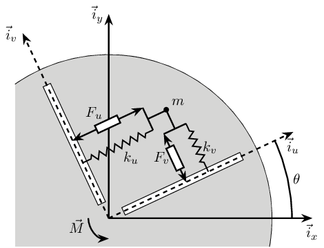
The system consists of one 2 degree of freedom translation stage on top of a spindle (figure fig:rotating_frame_2dof).
The control inputs are the forces applied by the actuators of the translation stage ($F_u$ and $F_v$). As the translation stage is rotating around the Z axis due to the spindle, the forces are applied along $u$ and $v$.
The measurement is either the $x-y$ displacement of the object located on top of the translation stage or the $u-v$ displacement of the sample with respect to a fixed reference frame.
In the following block diagram:
- $G$ is the transfer function from the forces applied in the actuators to the measurement
- $K$ is the controller to design
- $J$ is a Jacobian matrix usually used to change the reference frame
Indices $x$ and $y$ corresponds to signals in the fixed reference frame (along $\vec{i}_x$ and $\vec{i}_y$):
- $D_x$ is the measured position of the sample
- $r_x$ is the reference signal which corresponds to the wanted $D_x$
- $\epsilon_x$ is the position error
Indices $u$ and $v$ corresponds to signals in the rotating reference frame ($\vec{i}_u$ and $\vec{i}_v$):
- $F_u$ and $F_v$ are forces applied by the actuators
- $\epsilon_u$ and $\epsilon_v$ are position error of the sample along $\vec{i}_u$ and $\vec{i}_v$
Equations
<<sec:equations>> Based on the figure fig:rotating_frame_2dof, we can write the equations of motion of the system.
Let's express the kinetic energy $T$ and the potential energy $V$ of the mass $m$:
\begin{align} T & = \frac{1}{2} m \left( \dot{x}^2 + \dot{y}^2 \right) \\ V & = \frac{1}{2} k \left( x^2 + y^2 \right) \end{align}The Lagrangian is the kinetic energy minus the potential energy.
\begin{equation} L = T-V = \frac{1}{2} m \left( \dot{x}^2 + \dot{y}^2 \right) - \frac{1}{2} k \left( x^2 + y^2 \right) \end{equation}The partial derivatives of the Lagrangian with respect to the variables $(x, y)$ are:
\begin{align*} \frac{\partial L}{\partial x} & = -kx \\ \frac{\partial L}{\partial y} & = -ky \\ \frac{d}{dt}\frac{\partial L}{\partial \dot{x}} & = m\ddot{x} \\ \frac{d}{dt}\frac{\partial L}{\partial \dot{y}} & = m\ddot{y} \end{align*}The external forces applied to the mass are:
\begin{align*} F_{\text{ext}, x} &= F_u \cos{\theta} - F_v \sin{\theta}\\ F_{\text{ext}, y} &= F_u \sin{\theta} + F_v \cos{\theta} \end{align*}By appling the Lagrangian equations, we obtain:
\begin{align} m\ddot{x} + kx = F_u \cos{\theta} - F_v \sin{\theta}\\ m\ddot{y} + ky = F_u \sin{\theta} + F_v \cos{\theta} \end{align}We then change coordinates from $(x, y)$ to $(d_x, d_y, \theta)$.
\begin{align*} x & = d_u \cos{\theta} - d_v \sin{\theta}\\ y & = d_u \sin{\theta} + d_v \cos{\theta} \end{align*}We obtain:
\begin{align*} \ddot{x} & = \ddot{d_u} \cos{\theta} - 2\dot{d_u}\dot{\theta}\sin{\theta} - d_u\ddot{\theta}\sin{\theta} - d_u\dot{\theta}^2 \cos{\theta} - \ddot{d_v} \sin{\theta} - 2\dot{d_v}\dot{\theta}\cos{\theta} - d_v\ddot{\theta}\cos{\theta} + d_v\dot{\theta}^2 \sin{\theta} \\ \ddot{y} & = \ddot{d_u} \sin{\theta} + 2\dot{d_u}\dot{\theta}\cos{\theta} + d_u\ddot{\theta}\cos{\theta} - d_u\dot{\theta}^2 \sin{\theta} + \ddot{d_v} \cos{\theta} - 2\dot{d_v}\dot{\theta}\sin{\theta} - d_v\ddot{\theta}\sin{\theta} - d_v\dot{\theta}^2 \cos{\theta} \\ \end{align*}By injecting the previous result into the Lagrangian equation, we obtain:
\begin{align*} m \ddot{d_u} \cos{\theta} - 2m\dot{d_u}\dot{\theta}\sin{\theta} - m d_u\ddot{\theta}\sin{\theta} - m d_u\dot{\theta}^2 \cos{\theta} -m \ddot{d_v} \sin{\theta} - 2m\dot{d_v}\dot{\theta}\cos{\theta} - m d_v\ddot{\theta}\cos{\theta} + m d_v\dot{\theta}^2 \sin{\theta} + k d_u \cos{\theta} - k d_v \sin{\theta} = F_u \cos{\theta} - F_v \sin{\theta} \\ m \ddot{d_u} \sin{\theta} + 2m\dot{d_u}\dot{\theta}\cos{\theta} + m d_u\ddot{\theta}\cos{\theta} - m d_u\dot{\theta}^2 \sin{\theta} + m \ddot{d_v} \cos{\theta} - 2m\dot{d_v}\dot{\theta}\sin{\theta} - m d_v\ddot{\theta}\sin{\theta} - m d_v\dot{\theta}^2 \cos{\theta} + k d_u \sin{\theta} + k d_v \cos{\theta} = F_u \sin{\theta} + F_v \cos{\theta} \end{align*}Which is equivalent to:
\begin{align*} m \ddot{d_u} - 2m\dot{d_u}\dot{\theta}\frac{\sin{\theta}}{\cos{\theta}} - m d_u\ddot{\theta}\frac{\sin{\theta}}{\cos{\theta}} - m d_u\dot{\theta}^2 -m \ddot{d_v} \frac{\sin{\theta}}{\cos{\theta}} - 2m\dot{d_v}\dot{\theta} - m d_v\ddot{\theta} + m d_v\dot{\theta}^2 \frac{\sin{\theta}}{\cos{\theta}} + k d_u - k d_v \frac{\sin{\theta}}{\cos{\theta}} = F_u - F_v \frac{\sin{\theta}}{\cos{\theta}} \\ m \ddot{d_u} + 2m\dot{d_u}\dot{\theta}\frac{\cos{\theta}}{\sin{\theta}} + m d_u\ddot{\theta}\frac{\cos{\theta}}{\sin{\theta}} - m d_u\dot{\theta}^2 + m \ddot{d_v} \frac{\cos{\theta}}{\sin{\theta}} - 2m\dot{d_v}\dot{\theta} - m d_v\ddot{\theta} - m d_v\dot{\theta}^2 \frac{\cos{\theta}}{\sin{\theta}} + k d_u + k d_v \frac{\cos{\theta}}{\sin{\theta}} = F_u + F_v \frac{\cos{\theta}}{\sin{\theta}} \end{align*}We can then subtract and add the previous equations to obtain the following equations:
We obtain two differential equations that are coupled through:
- Euler forces: $m d_v \ddot{\theta}$
- Coriolis forces: $2 m \dot{d_v} \dot{\theta}$
Without the coupling terms, each equation is the equation of a one degree of freedom mass-spring system with mass $m$ and stiffness $k- m\dot{\theta}^2$. Thus, the term $- m\dot{\theta}^2$ acts like a negative stiffness (due to centrifugal forces).
The forces induced by the rotating reference frame are independent of the stiffness of the actuator. The resulting effect of those forces should then be higher when using softer actuators.
Numerical Values for the NASS
Let's define the parameters for the NASS.
| Light sample mass [kg] | 3.5e+01 |
| Heavy sample mass [kg] | 8.5e+01 |
| Max rot. speed - light [rpm] | 6.0e+01 |
| Max rot. speed - heavy [rpm] | 1.0e+00 |
| Voice Coil Stiffness [N/m] | 1.0e+03 |
| Piezo Stiffness [N/m] | 1.0e+08 |
| Max rot. acceleration [rad/s2] | 1.0e+00 |
| Max mass excentricity [m] | 1.0e-02 |
| Max Horizontal speed [m/s] | 2.0e-01 |
Euler and Coriolis forces - Numerical Result
First we will determine the value for Euler and Coriolis forces during regular experiment.
- Euler forces: $m d_v \ddot{\theta}$
- Coriolis forces: $2 m \dot{d_v} \dot{\theta}$
The obtained values are displayed in table tab:euler_coriolis.
| Light | Heavy | |
|---|---|---|
| Coriolis | 88.0N | 3.6N |
| Euler | 0.4N | 0.8N |
Negative Spring Effect - Numerical Result
The negative stiffness due to the rotation is equal to $-m{\omega_0}^2$.
The values for the negative spring effect are displayed in table tab:negative_spring.
This is definitely negligible when using piezoelectric actuators. It may not be the case when using voice coil actuators.
| Light | Heavy | |
|---|---|---|
| Neg. Spring | 1381.7[N/m] | 0.9[N/m] |
Limitations due to coupling
To simplify, we consider a constant rotating speed $\dot{\theta} = {\omega_0}$ and thus $\ddot{\theta} = 0$.
From equations eq:du_coupled and eq:dv_coupled, we obtain:
\begin{align*} (m s^2 + (k - m{\omega_0}^2)) d_u &= F_u + 2 m {\omega_0} s d_v \\ (m s^2 + (k - m{\omega_0}^2)) d_v &= F_v - 2 m {\omega_0} s d_u \\ \end{align*}From second equation: \[ d_v = \frac{1}{m s^2 + (k - m{\omega_0}^2)} F_v - \frac{2 m {\omega_0} s}{m s^2 + (k - m{\omega_0}^2)} d_u \]
And we re-inject $d_v$ into the first equation:
\begin{equation*} (m s^2 + (k - m{\omega_0}^2)) d_u = F_u + \frac{2 m {\omega_0} s}{m s^2 + (k - m{\omega_0}^2)} F_v - \frac{(2 m {\omega_0} s)^2}{m s^2 + (k - m{\omega_0}^2)} d_u \end{equation*} \begin{equation*} \frac{(m s^2 + (k - m{\omega_0}^2))^2 + (2 m {\omega_0} s)^2}{m s^2 + (k - m{\omega_0}^2)} d_u = F_u + \frac{2 m {\omega_0} s}{m s^2 + (k - m{\omega_0}^2)} F_v \end{equation*}Finally we obtain $d_u$ function of $F_u$ and $F_v$. \[ d_u = \frac{m s^2 + (k - m{\omega_0}^2)}{(m s^2 + (k - m{\omega_0}^2))^2 + (2 m {\omega_0} s)^2} F_u + \frac{2 m {\omega_0} s}{(m s^2 + (k - m{\omega_0}^2))^2 + (2 m {\omega_0} s)^2} F_v \]
Similarly we can obtain $d_v$ function of $F_u$ and $F_v$: \[ d_v = \frac{m s^2 + (k - m{\omega_0}^2)}{(m s^2 + (k - m{\omega_0}^2))^2 + (2 m {\omega_0} s)^2} F_v - \frac{2 m {\omega_0} s}{(m s^2 + (k - m{\omega_0}^2))^2 + (2 m {\omega_0} s)^2} F_u \]
The two previous equations can be written in a matrix form:
Then, coupling is negligible if $|-m \omega^2 + (k - m{\omega_0}^2)| \gg |2 m {\omega_0} \omega|$.
Numerical Analysis
We plot on the same graph $\frac{|-m \omega^2 + (k - m {\omega_0}^2)|}{|2 m \omega_0 \omega|}$ for the voice coil and the piezo:
- with the light sample (figure fig:coupling_light).
- with the heavy sample (figure fig:coupling_heavy).
<<plt-matlab>>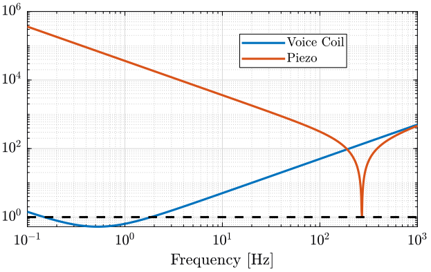
<<plt-matlab>>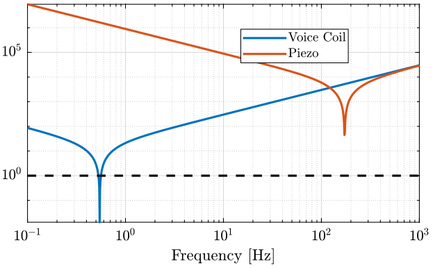
Coupling is higher for actuators with small stiffness.
Limitations due to negative stiffness effect
If $\max{\dot{\theta}} \ll \sqrt{\frac{k}{m}}$, then the negative spring effect is negligible and $k - m\dot{\theta}^2 \approx k$.
Let's estimate what is the maximum rotation speed for which the negative stiffness effect is still negligible ($\omega_\text{max} = 0.1 \sqrt{\frac{k}{m}}$). Results are shown table tab:negative_stiffness.
| Voice Coil | Piezo | |
|---|---|---|
| Light | 5[rpm] | 1614[rpm] |
| Heavy | 3[rpm] | 1036[rpm] |
The negative spring effect is proportional to the rotational speed $\omega$. The system dynamics will be much more affected when using soft actuator.
Negative stiffness effect has very important effect when using soft actuators.
The system can even goes unstable when $m \omega^2 > k$, that is when the centrifugal forces are higher than the forces due to stiffness.
From this analysis, we can determine the lowest practical stiffness that is possible to use: $k_\text{min} = 10 m \omega^2$ (table tab:min_k)
| Light | Heavy | |
|---|---|---|
| k min [N/m] | 2199 | 89 |
Effect of rotation speed on the plant
As shown in equation eq:coupledplant, the plant changes with the rotation speed $\omega_0$.
Then, we compute the bode plot of the direct term and coupling term for multiple rotating speed.
Then we compare the result between voice coil and piezoelectric actuators.
Voice coil actuator
<<plt-matlab>>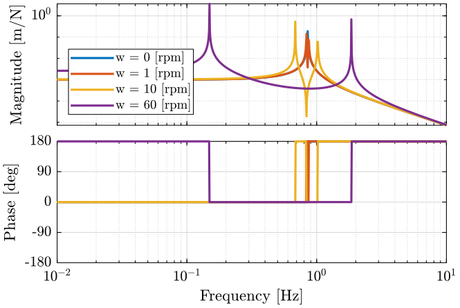
<<plt-matlab>>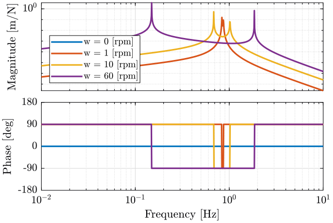
Piezoelectric actuator
<<plt-matlab>>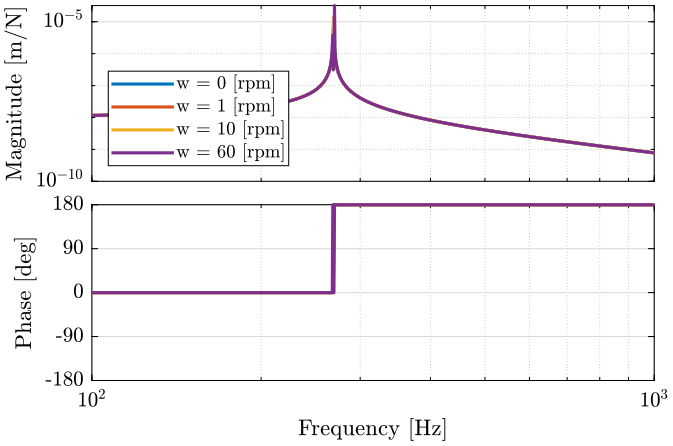
<<plt-matlab>>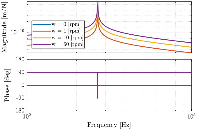
Analysis
When the rotation speed is null, the coupling terms are equal to zero and the diagonal terms corresponds to one degree of freedom mass spring system.
When the rotation speed in not null, the resonance frequency is duplicated into two pairs of complex conjugate poles.
As the rotation speed increases, one of the two resonant frequency goes to lower frequencies as the other one goes to higher frequencies.
The poles of the coupling terms are the same as the poles of the diagonal terms. The magnitude of the coupling terms are increasing with the rotation speed.
As shown in the previous figures, the system with voice coil is much more sensitive to rotation speed.
Campbell diagram
The poles of the system are computed for multiple values of the rotation frequency. To simplify the computation of the poles, we add some damping to the system.
  m = mlight;
  k = kvc;
  c = 0.1*sqrt(k*m);

  ws = linspace(0, 10, 100); % [rad/s]

  polesvc = zeros(2, length(ws));

  for i = 1:length(ws)
    polei = pole(1/((m*s^2 + c*s + (k - m*ws(i)^2))^2 + (2*m*ws(i)*s)^2));
    polesvc(:, i) = sort(polei(imag(polei) > 0));
  end
m = mlight;
k = kpz;
c = 0.1*sqrt(k*m);
ws = linspace(0, 1000, 100); % [rad/s]
polespz = zeros(2, length(ws));
for i = 1:length(ws)
polei = pole(1/((m*s^2 + c*s + (k - m*ws(i)^2))^2 + (2*m*ws(i)*s)^2));
polespz(:, i) = sort(polei(imag(polei) > 0));
endWe then plot the real and imaginary part of the poles as a function of the rotation frequency (figures fig:poles_w_vc and fig:poles_w_pz).
When the real part of one pole becomes positive, the system goes unstable.
For the voice coil (figure fig:poles_w_vc), the system is unstable when the rotation speed is above 5 rad/s. The real and imaginary part of the poles of the system with piezoelectric actuators are changing much less (figure fig:poles_w_pz).
<<plt-matlab>>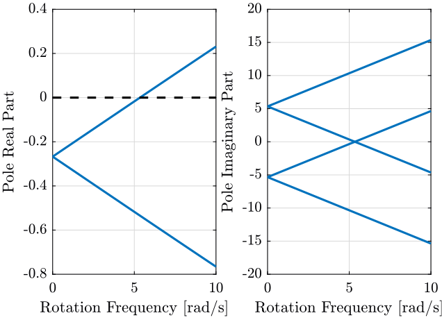
<<plt-matlab>>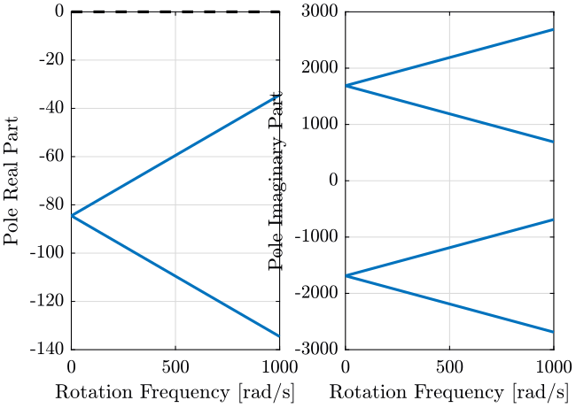
Control Strategies
<<sec:control_strategies>>
Measurement in the fixed reference frame
First, let's consider a measurement in the fixed referenced frame.
The transfer function from actuator $[F_u, F_v]$ to sensor $[D_x, D_y]$ is then $G(\theta)$.
Then the measurement is subtracted to the reference signal $[r_x, r_y]$ to obtain the position error in the fixed reference frame $[\epsilon_x, \epsilon_y]$.
The position error $[\epsilon_x, \epsilon_y]$ is then express in the rotating frame corresponding to the actuators $[\epsilon_u, \epsilon_v]$.
Finally, the control low $K$ links the position errors $[\epsilon_u, \epsilon_v]$ to the actuator forces $[F_u, F_v]$.
The block diagram is shown on figure fig:control_measure_fixed_2dof.
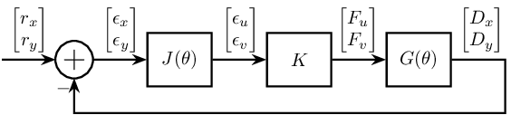
The loop gain is then $L = G(\theta) K J(\theta)$.
One question we wish to answer is: is $G(\theta) J(\theta) = G(\theta_0) J(\theta_0)$?
Measurement in the rotating frame
Let's consider that the measurement is made in the rotating reference frame.
The corresponding block diagram is shown figure fig:control_measure_rotating_2dof
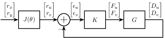
The loop gain is $L = G K$.
Multi Body Model - Simscape
<<sec:simscape>>
Initialization
First we define the parameters that must be defined in order to run the Simscape simulation.
  w = 2*pi; % Rotation speed [rad/s]

  theta_e = 0; % Static measurement error on the angle theta [rad]

  m = 5; % mass of the sample [kg]

  mTuv = 30;% Mass of the moving part of the Tuv stage [kg]
  kTuv = 1e8; % Stiffness of the Tuv stage [N/m]
  cTuv = 0; % Damping of the Tuv stage [N/(m/s)]
Then, we defined parameters that will be used in the following analysis.
  mlight = 5; % Mass for light sample [kg]
  mheavy = 55; % Mass for heavy sample [kg]

  wlight = 2*pi; % Max rot. speed for light sample [rad/s]
  wheavy = 2*pi/60; % Max rot. speed for heavy sample [rad/s]

  kvc = 1e3; % Voice Coil Stiffness [N/m]
  kpz = 1e8; % Piezo Stiffness [N/m]

  d = 0.01; % Maximum excentricity from rotational axis [m]

  freqs = logspace(-2, 3, 1000); % Frequency vector for analysis [Hz]
Identification in the rotating referenced frame
We initialize the inputs and outputs of the system to identify:
- Inputs: $f_u$ and $f_v$
- Outputs: $d_u$ and $d_v$
  %% Options for Linearized
  options = linearizeOptions;
  options.SampleTime = 0;

  %% Name of the Simulink File
  mdl = 'rotating_frame';

  %% Input/Output definition
  io(1) = linio([mdl, '/fu'], 1, 'input');
  io(2) = linio([mdl, '/fv'], 1, 'input');

  io(3) = linio([mdl, '/du'], 1, 'output');
  io(4) = linio([mdl, '/dv'], 1, 'output');
We start we identify the transfer functions at high speed with the light sample.
  w = wlight; % Rotation speed [rad/s]
  m = mlight; % mass of the sample [kg]

  kTuv = kpz;
  Gpz_light = linearize(mdl, io, 0.1);
  Gpz_light.InputName  = {'Fu', 'Fv'};
  Gpz_light.OutputName = {'Du', 'Dv'};

  kTuv = kvc;
  Gvc_light = linearize(mdl, io, 0.1);
  Gvc_light.InputName  = {'Fu', 'Fv'};
  Gvc_light.OutputName = {'Du', 'Dv'};
Then we identify the system with an heavy mass and low speed.
  w = wheavy; % Rotation speed [rad/s]
  m = mheavy; % mass of the sample [kg]

  kTuv = kpz;
  Gpz_heavy = linearize(mdl, io, 0.1);
  Gpz_heavy.InputName  = {'Fu', 'Fv'};
  Gpz_heavy.OutputName = {'Du', 'Dv'};

  kTuv = kvc;
  Gvc_heavy = linearize(mdl, io, 0.1);
  Gvc_heavy.InputName  = {'Fu', 'Fv'};
  Gvc_heavy.OutputName = {'Du', 'Dv'};
Coupling ratio between $f_{uv}$ and $d_{uv}$
In order to validate the equations written, we can compute the coupling ratio using the simscape model and compare with the equations.
From the previous identification, we plot the coupling ratio in both case (figure fig:coupling_ratio_light_heavy).
We obtain the same result than the analytical case (figures fig:coupling_light and fig:coupling_heavy).
<<plt-matlab>>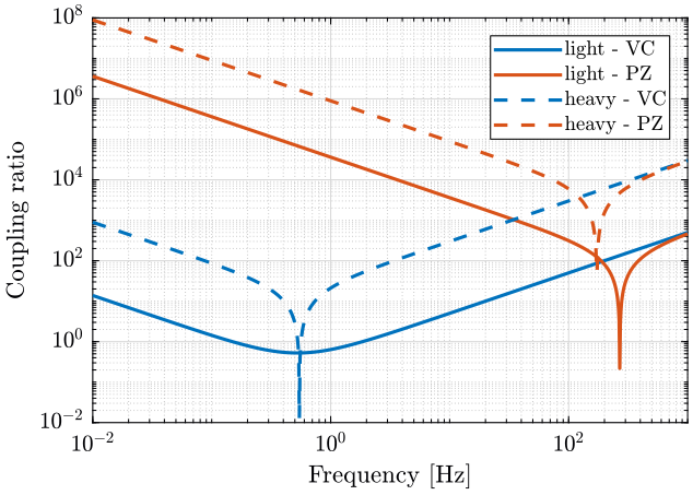
Plant Control
The goal is to study the control problems due to the coupling that appears because of the rotation.
First, we identify the system when the rotation speed is null and then when the rotation speed is equal to 60rpm.
The actuators are voice coil with some damping added.
The bode plot of the system not rotating and rotating at 60rpm is shown figure fig:Gvc_speed.
<<plt-matlab>>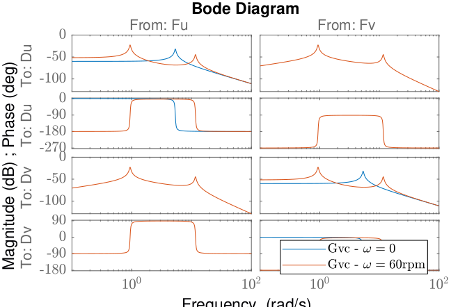
Controller design
We design a controller based on the identification when the system is not rotating.
sisotool(Gvc('Du', 'fu'))The controller is a lead-lag controller with the following transfer function.
  Kll = 2.0698e09*(s+40.45)*(s+1.181)/(s*(s+198.4)*(s+2790));
  K = [Kll 0;
       0   Kll];
The loop gain is displayed figure fig:Gvc_loop_gain.
<<plt-matlab>>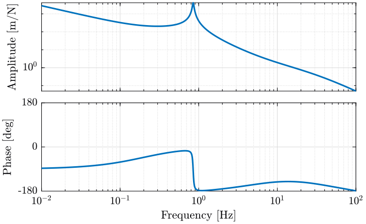
Controlling the rotating system
We here want to see if the system is robust with respect to the rotation speed. We then use the controller based on the non-rotating system, and see if the system is stable and its dynamics.
We can then plot the same loop gain with the rotating system using the same controller (figure fig:Gtvc_loop_gain). The result obtained is unstable.
<<plt-matlab>>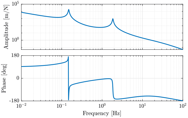
We can look at the poles of the system where we control only one direction ($u$ for instance). We obtain a pole with a positive real part.
pole(feedback(Gtvc, blkdiag(Kll, 0)))| -2798 |
| -58.906+94.246i |
| -58.906-94.246i |
| -71.654 |
| 3.1648 |
| -3.3031 |
| -1.1902 |
However, when we look at the poles of the closed loop with a diagonal controller, all the poles have negative real part and the system is stable.
pole(feedback(Gtvc, blkdiag(Kll, Kll)))| -2798+0.035765i |
| -2798-0.035765i |
| -56.406+105.34i |
| -56.406-105.34i |
| -64.482+79.308i |
| -64.482-79.308i |
| -68.521+13.503i |
| -68.521-13.503i |
| -1.1837+0.0041777i |
| -1.1837-0.0041777i |
*
  figure;
bode(Kll*Gvc('Du', 'fu')) sisotool(Gtvc('Du', 'fu'), Kll) figure;
bode(Kll*Gtvc('Du', 'fu')) Gcl = feedback(Gvc, K); Gtcl = feedback(Gtvc, K); figure;
bode(Gcl, Gtcl)test
<<plt-matlab>>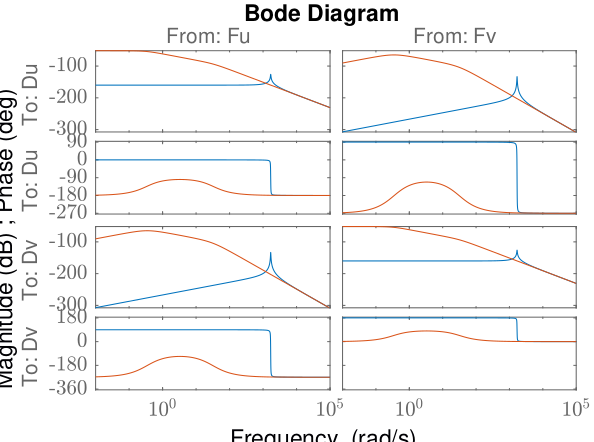
And then with the heavy sample.
  rot_speed = wheavy;
  angle_e = 0;
  m = mheavy;

  k = kpz;
  c = 1e3;
  Gpz_heavy = linearize(mdl, io, 0.1);

  k = kvc;
  c = 1e3;
  Gvc_heavy = linearize(mdl, io, 0.1);

  Gpz_heavy.InputName  = {'Fu', 'Fv'};
  Gpz_heavy.OutputName = {'Du', 'Dv'};
  Gvc_heavy.InputName  = {'Fu', 'Fv'};
Gvc_heavy.OutputName = {'Du', 'Dv'}; <<plt-matlab>>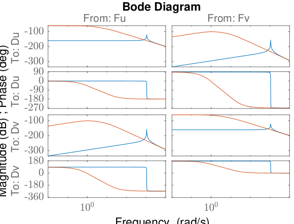
Plot the ratio between the main transfer function and the coupling term:
<<plt-matlab>>
<<plt-matlab>>
Low rotation speed and High rotation speed
  rot_speed = 2*pi/60; angle_e = 0;
  G_low = linearize(mdl, io, 0.1);

  rot_speed = 2*pi; angle_e = 0;
  G_high = linearize(mdl, io, 0.1);

  G_low.InputName  = {'Fu', 'Fv'};
  G_low.OutputName = {'Du', 'Dv'};
  G_high.InputName  = {'Fu', 'Fv'};
G_high.OutputName = {'Du', 'Dv'}; figure;
bode(G_low, G_high);Identification in the fixed frame
Let's define some options as well as the inputs and outputs for linearization.
  %% Options for Linearized
  options = linearizeOptions;
  options.SampleTime = 0;

  %% Name of the Simulink File
  mdl = 'rotating_frame';

  %% Input/Output definition
  io(1) = linio([mdl, '/fx'], 1, 'input');
  io(2) = linio([mdl, '/fy'], 1, 'input');

  io(3) = linio([mdl, '/dx'], 1, 'output');
  io(4) = linio([mdl, '/dy'], 1, 'output');
We then define the error estimation of the error and the rotational speed.
  %% Run the linearization
  angle_e = 0;
  rot_speed = 0;
Finally, we run the linearization.
  G = linearize(mdl, io, 0);

  %% Input/Output names
  G.InputName  = {'Fx', 'Fy'};
  G.OutputName = {'Dx', 'Dy'};
%% Run the linearization
angle_e = 0;
rot_speed = 2*pi;
Gr = linearize(mdl, io, 0);
%% Input/Output names
Gr.InputName = {'Fx', 'Fy'};
Gr.OutputName = {'Dx', 'Dy'}; %% Run the linearization
angle_e = 1*2*pi/180;
rot_speed = 2*pi;
Ge = linearize(mdl, io, 0);
%% Input/Output names
Ge.InputName = {'Fx', 'Fy'};
Ge.OutputName = {'Dx', 'Dy'}; figure;
bode(G);
% exportFig('G_x_y', 'wide-tall');
figure;
bode(Ge);
% exportFig('G_x_y_e', 'normal-normal');Identification from actuator forces to displacement in the fixed frame
  %% Options for Linearized
  options = linearizeOptions;
  options.SampleTime = 0;

  %% Name of the Simulink File
  mdl = 'rotating_frame';

  %% Input/Output definition
  io(1) = linio([mdl, '/fu'], 1, 'input');
  io(2) = linio([mdl, '/fv'], 1, 'input');

  io(3) = linio([mdl, '/dx'], 1, 'output');
  io(4) = linio([mdl, '/dy'], 1, 'output');
rot_speed = 2*pi;
angle_e = 0;
G = linearize(mdl, io, 0.0);
G.InputName = {'Fu', 'Fv'};
G.OutputName = {'Dx', 'Dy'}; rot_speed = 2*pi;
angle_e = 0;
G1 = linearize(mdl, io, 0.4);
G1.InputName = {'Fu', 'Fv'};
G1.OutputName = {'Dx', 'Dy'}; rot_speed = 2*pi;
angle_e = 0;
G2 = linearize(mdl, io, 0.8);
G2.InputName = {'Fu', 'Fv'};
G2.OutputName = {'Dx', 'Dy'}; figure;
bode(G, G1, G2);
exportFig('G_u_v_to_x_y', 'wide-tall');Effect of the rotating Speed
<<sec:effect_rot_speed>>
TODO Use realistic parameters for the mass of the sample and stiffness of the X-Y stage
TODO Check if the plant is changing a lot when we are not turning to when we are turning at the maximum speed (60rpm)
Effect of the X-Y stage stiffness
<<sec:effect_stiffness>>
TODO At full speed, check how the coupling changes with the stiffness of the actuators
Control Implementation
<<sec:control>>