phd-nass-rotating-3dof-model/nass-rotating-3dof-model.org

NASS - Effect of rotation

• Introduction
• System Description and Analysis
  • Introduction
  • Equations of motion
  • Transfer Functions in the Laplace domain
  • System Poles: Campbell Diagram
  • System Dynamics: Effect of rotation
• Integral Force Feedback
  • Introduction
  • System and Equations of motion
  • Effect of the rotation speed on the IFF plant dynamics
  • Decentralized Integral Force Feedback
• Integral Force Feedback with an High Pass Filter
  • Introduction
  • Modified Integral Force Feedback Controller
  • Optimal IFF with HPF parameters $\omega_i$ and $g$
  • Obtained Damped Plant
• IFF with a stiffness in parallel with the force sensor
  • Introduction
  • Equations
  • Effect of the parallel stiffness on the IFF plant
  • Effect of $k_p$ on the attainable damping
  • Damped plant
• Relative Damping Control
  • Introduction
  • Equations of motion
  • Decentralized Relative Damping Control
  • Damped Plant
• Comparison of Active Damping Techniques
  • Introduction
  • Root Locus
  • Obtained Damped Plant
  • Transmissibility And Compliance
• Rotating Nano-Hexapod
  • Introduction
  • Nano-Active-Stabilization-System - Plant Dynamics
  • Optimal IFF with High Pass Filter
  • Optimal IFF with Parallel Stiffness
  • Optimal Relative Motion Control
  • Comparison of the obtained damped plants
• Nano-Active-Stabilization-System with rotation
  • Introduction
  • NASS model
  • System dynamics
  • Effect of disturbances
• Conclusion
• Bibliography

---

This report is also available as a pdf.

---

Introduction   ignore

An important aspect of the Nano Active Stabilization System (NASS) is that the nano-hexapod is continuously rotating around a vertical axis while the external metrology is not. Such rotation induces gyroscopic effects that may impact the system dynamics and obtained performances.

In this report, this rotating aspect of the NASS is studied. It is structured in several sections:

• Section ref:sec:rotating_system_description: a simple model of a rotating suspended platform that will be used throughout this study is presented. The effect of the rotation velocity on the system dynamics is shown.
• Section ref:sec:rotating_iff_pure_int: Integral Force Feedback (IFF) is applied to the rotating platform, and it is shown that the unconditional stability of IFF is lost due to Gyroscopic effects induced by the rotation.
• Section ref:sec:rotating_iff_pseudo_int: A first modification of the IFF control law is proposed such that damping can be added to the suspension modes in a robust way. This modification consists of adding an high pass filter to the IFF controller. Optimal high pass filter cut-off frequency is computed.
• Section ref:sec:rotating_iff_parallel_stiffness: A second modification is proposed to regain the unconditional stability of IFF. This modification consists of adding stiffness in parallel to the force sensors. Optimal parallel stiffness is computed.
• Section ref:sec:rotating_relative_damp_control: Relative damping control is applied to the rotating system.
• Section ref:sec:rotating_comp_act_damp: Once the optimal control parameters for the three tested active damping techniques are obtained, they are compared in terms of achievable damping, obtained damped plant and closed-loop compliance and transmissibility.
• Section ref:sec:rotating_nano_hexapod: the previous analysis is applied on three nano-hexapod stiffnesses and optimal active damping controller are obtained.
• Section ref:sec:rotating_nass: up until this section, the study was performed on a very simplistic model that just captures the rotation aspect and the model parameters were not tuned to corresponds to the NASS. In this last section, a model of the micro-station is added below the suspended platform (i.e. the nano-hexapod) with a rotating spindle and parameters tuned to match the NASS dynamics. The goal is to determine if the rotation imposes performance limitation for the NASS.

To run the Matlab code, go in the matlab directory and run the Matlab files corresponding to each section (see Table ref:tab:section_matlab_code).

Sections	Matlab File
Section ref:sec:rotating_system_description	rotating_1_system_description.m
Section ref:sec:rotating_iff_pure_int	rotating_2_iff_pure_int.m
Section ref:sec:rotating_iff_pseudo_int	rotating_3_iff_hpf.m
Section ref:sec:rotating_iff_parallel_stiffness	rotating_4_iff_kp.m
Section ref:sec:rotating_relative_damp_control	rotating_5_rdc.m
Section ref:sec:rotating_comp_act_damp	rotating_5_act_damp_comparison.m
Section ref:sec:rotating_nano_hexapod	rotating_6_nano_hexapod.m
Section ref:sec:rotating_nass	rotating_6_nass.m

System Description and Analysis

<<sec:rotating_system_description>>

Introduction   ignore

The studied system consists of a 2 degree of freedom translation stage on top of a rotating stage (Figure ref:fig:rotating_3dof_model_schematic).

The rotating stage is supposed to be ideal, meaning it induces a perfect rotation $\theta(t) = \Omega t$ where $\Omega$ is the rotational speed in $\si{\radian\per\s}$.

The suspended platform consists of two orthogonal actuators each represented by three elements in parallel: a spring with a stiffness $k$ in $\si{\newton\per\meter}$, a dashpot with a damping coefficient $c$ in $\si{\newton\per(\meter\per\second)}$ and an ideal force source $F_u, F_v$. A payload with a mass $m$ in $\si{\kilo\gram}$, is mounted on the (rotating) suspended platform.

Two reference frames are used: an inertial frame $(\vec{i}_x, \vec{i}_y, \vec{i}_z)$ and a uniform rotating frame $(\vec{i}_u, \vec{i}_v, \vec{i}_w)$ rigidly fixed on top of the rotating stage with $\vec{i}_w$ aligned with the rotation axis. The position of the payload is represented by $(d_u, d_v, 0)$ expressed in the rotating frame.

\begin{tikzpicture}
  % Angle
  \def\thetau{25}

  % Rotational Stage
  \draw[fill=black!60!white] (0, 0) circle (4.3);
  \draw[fill=black!40!white] (0, 0) circle (3.8);

  % Label
  \node[anchor=north west, rotate=\thetau] at (-2.5, 2.5) {\small Rotating Stage};

  % Rotating Scope
  \begin{scope}[rotate=\thetau]
    % Rotating Frame
    \draw[fill=black!20!white] (-2.6, -2.6) rectangle (2.6, 2.6);
    % Label
    \node[anchor=north west, rotate=\thetau] at (-2.6, 2.6) {\small Suspended Platform};

    % Mass
    \draw[fill=white] (-1, -1) rectangle (1, 1);
    % Label
    \node[anchor=south west, rotate=\thetau] at (-1, -1) {\small Payload};

    % Attached Points
    \node[] at (-1, 0){$\bullet$};
    \draw[] (-1, 0) -- ++(-0.2, 0) coordinate(cu);
    \draw[] ($(cu) + (0, -0.8)$) coordinate(actu) -- ($(cu) + (0, 0.8)$) coordinate(ku);
    \node[] at (0, -1){$\bullet$};
    \draw[] (0, -1) -- ++(0, -0.2) coordinate(cv);
    \draw[] ($(cv) + (-0.8, 0)$)coordinate(kv) -- ($(cv) + (0.8, 0)$) coordinate(actv);

    % Spring and Actuator for U
    \draw[actuator={0.6}{0.2}{black}] (actu) -- node[above=0.1, rotate=\thetau]{$F_u$} (actu-|-2.6,0);
    \draw[spring=0.2] (ku) -- node[above=0.1, rotate=\thetau]{$k$} (ku-|-2.6,0);
    \draw[damper={black}{8}{8}] (cu) -- node[above left=0.2 and -0.1, rotate=\thetau]{$c$} (cu-|-2.6,0);

    \draw[actuator={0.6}{0.2}{black}] (actv) -- node[left, rotate=\thetau]{$F_v$} (actv|-0,-2.6);
    \draw[spring=0.2] (kv) -- node[left, rotate=\thetau]{$k$} (kv|-0,-2.6);
    \draw[damper={black}{8}{8}] (cv) -- node[left=0.1, rotate=\thetau]{$c$} (cv|-0,-2.6);
  \end{scope}

  % Inertial Frame
  \draw[->] (-4, -4) -- ++(2, 0) node[below]{$\vec{i}_x$};
  \draw[->] (-4, -4) -- ++(0, 2) node[left]{$\vec{i}_y$};
  \draw[fill, color=black] (-4, -4) circle (0.06);
  \node[draw, circle, inner sep=0pt, minimum size=0.3cm, label=left:$\vec{i}_z$] at (-4, -4){};

  \draw[->] (0, 0) node[above left, rotate=\thetau]{$\vec{i}_w$} -- ++(\thetau:2) node[above, rotate=\thetau]{$\vec{i}_u$};
  \draw[->] (0, 0) -- ++(\thetau+90:2) node[left, rotate=\thetau]{$\vec{i}_v$};
  \draw[fill, color=black] (0,0) circle (0.06);
  \node[draw, circle, inner sep=0pt, minimum size=0.3cm] at (0, 0){};
  \draw[dashed] (0, 0) -- ++(2, 0);
  \draw[] (1.5, 0) arc (0:\thetau:1.5) node[midway, right]{$\theta$};

  \draw[->] (3.5, 0) arc (0:40:3.5) node[midway, left]{$\Omega$};
\end{tikzpicture}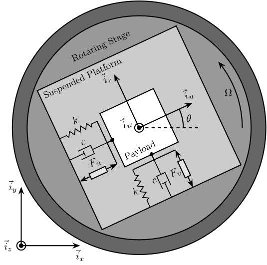

Schematic of the studied system

Equations of motion

To obtain the equations of motion for the system represented in Figure ref:fig:rotating_3dof_model_schematic, the Lagrangian equations are used:

\begin{equation} \frac{d}{dt} \left( \frac{\partial L}{\partial \dot{q}_i} \right) + \frac{\partial D}{\partial \dot{q}_i} - \frac{\partial L}{\partial q_i} = Q_i \end{equation}

with $L = T - V$ the Lagrangian, $T$ the kinetic coenergy, $V$ the potential energy, $D$ the dissipation function, and $Q_i$ the generalized force associated with the generalized variable $\begin{bmatrix}q_1 & q_2\end{bmatrix} = \begin{bmatrix}d_u & d_v\end{bmatrix}$. The equation of motion corresponding to the constant rotation along $\vec{i}_w$ is disregarded as this motion is considered to be imposed by the rotation stage.

\begin{equation} \begin{aligned} T &= \frac{1}{2} m \left( ( \dot{d}_u - \Omega d_v )^2 + ( \dot{d}_v + \Omega d_u )^2 \right), \\ V &= \frac{1}{2} k \big( {d_u}^2 + {d_v}^2 \big), \ Q_1 = F_u, \\ D &= \frac{1}{2} c \big( \dot{d}_u{}^2 + \dot{d}_v{}^2 \big), \ Q_2 = F_v \end{aligned} \end{equation}

Substituting equations eqref:eq:energy_functions_lagrange into equation eqref:eq:lagrangian_equations for both generalized coordinates gives two coupled differential equations eqref:eq:eom_coupled_1 and eqref:eq:eom_coupled_2.

\begin{subequations} \begin{align} m \ddot{d}_u + c \dot{d}_u + ( k - m \Omega^2 ) d_u &= F_u + 2 m \Omega \dot{d}_v \label{eq:eom_coupled_1} \\ m \ddot{d}_v + c \dot{d}_v + ( k \underbrace{-\,m \Omega^2}_{\text{Centrif.}} ) d_v &= F_v \underbrace{-\,2 m \Omega \dot{d}_u}_{\text{Coriolis}} \label{eq:eom_coupled_2} \end{align} \end{subequations}

The uniform rotation of the system induces two gyroscopic effects as shown in equation eqref:eq:eom_coupled:

• Centrifugal forces: that can been seen as an added negative stiffness $- m \Omega^2$ along $\vec{i}_u$ and $\vec{i}_v$
• Coriolis Forces: that adds coupling between the two orthogonal directions.

One can verify that without rotation ($\Omega = 0$) the system becomes equivalent to two uncoupled one degree of freedom mass-spring-damper systems.

Transfer Functions in the Laplace domain

To study the dynamics of the system, the differential equations of motions eqref:eq:eom_coupled are converted into the Laplace domain and the $2 \times 2$ transfer function matrix $\mathbf{G}_d$ from $\begin{bmatrix}F_u & F_v\end{bmatrix}$ to $\begin{bmatrix}d_u & d_v\end{bmatrix}$ in equation eqref:eq:Gd_mimo_tf is obtained. Its elements are shown in equation eqref:eq:Gd_indiv_el.

\begin{equation} \begin{bmatrix} d_u \\ d_v \end{bmatrix} = \mathbf{G}_d \begin{bmatrix} F_u \\ F_v \end{bmatrix} \end{equation} \begin{subequations} \begin{align} \mathbf{G}_{d}(1,1) &= \mathbf{G}_{d}(2,2) = \frac{ms^2 + cs + k - m \Omega^2}{\left( m s^2 + cs + k - m \Omega^2 \right)^2 + \left( 2 m \Omega s \right)^2} \\ \mathbf{G}_{d}(1,2) &= -\mathbf{G}_{d}(2,1) = \frac{2 m \Omega s}{\left( m s^2 + cs + k - m \Omega^2 \right)^2 + \left( 2 m \Omega s \right)^2} \end{align} \end{subequations}

To simplify the analysis, the undamped natural frequency $\omega_0$ and the damping ratio $\xi$ are used as in equation eqref:eq:xi_and_omega.

\begin{equation} \omega_0 = \sqrt{\frac{k}{m}} \text{ in } \si{\radian\per\second}, \quad \xi = \frac{c}{2 \sqrt{k m}} \end{equation}

The elements of transfer function matrix $\mathbf{G}_d$ are now described by equation eqref:eq:Gd_w0_xi_k.

\begin{subequations} \begin{align} \mathbf{G}_{d}(1,1) &= \frac{\frac{1}{k} \left( \frac{s^2}{{\omega_0}^2} + 2 \xi \frac{s}{\omega_0} + 1 - \frac{{\Omega}^2}{{\omega_0}^2} \right)}{\left( \frac{s^2}{{\omega_0}^2} + 2 \xi \frac{s}{\omega_0} + 1 - \frac{{\Omega}^2}{{\omega_0}^2} \right)^2 + \left( 2 \frac{\Omega}{\omega_0} \frac{s}{\omega_0} \right)^2} \\ \mathbf{G}_{d}(1,2) &= \frac{\frac{1}{k} \left( 2 \frac{\Omega}{\omega_0} \frac{s}{\omega_0} \right)}{\left( \frac{s^2}{{\omega_0}^2} + 2 \xi \frac{s}{\omega_0} + 1 - \frac{{\Omega}^2}{{\omega_0}^2} \right)^2 + \left( 2 \frac{\Omega}{\omega_0} \frac{s}{\omega_0} \right)^2} \end{align} \end{subequations}

System Poles: Campbell Diagram

The poles of $\mathbf{G}_d$ are the complex solutions $p$ of equation eqref:eq:poles.

\begin{equation} \left( \frac{p^2}{{\omega_0}^2} + 2 \xi \frac{p}{\omega_0} + 1 - \frac{{\Omega}^2}{{\omega_0}^2} \right)^2 + \left( 2 \frac{\Omega}{\omega_0} \frac{p}{\omega_0} \right)^2 = 0 \end{equation}

Supposing small damping ($\xi \ll 1$), two pairs of complex conjugate poles are obtained as shown in equation eqref:eq:pole_values.

\begin{subequations} \begin{align} p_{+} &= - \xi \omega_0 \left( 1 + \frac{\Omega}{\omega_0} \right) \pm j \omega_0 \left( 1 + \frac{\Omega}{\omega_0} \right) \\ p_{-} &= - \xi \omega_0 \left( 1 - \frac{\Omega}{\omega_0} \right) \pm j \omega_0 \left( 1 - \frac{\Omega}{\omega_0} \right) \end{align} \end{subequations}

%% Model parameters for first analysis
kn = 1;    % Actuator Stiffness [N/m]
mn = 1;    % Payload Mass [kg]
cn = 0.05; % Actuator Damping [N/(m/s)]

xin = cn/(2*sqrt(kn*mn)); % Modal Damping [-]
w0n = sqrt(kn/mn);       % Natural Frequency [rad/s]

%% Computation of the poles as a function of the rotating velocity
Wzs = linspace(0, 2, 51); % Vector of rotation speeds [rad/s]

p_ws = zeros(4, length(Wzs));

for i = 1:length(Wzs)
    Wz = Wzs(i);

    pole_G = pole(1/(((s^2)/(w0n^2) + 2*xin*s/w0n + 1 - (Wz^2)/(w0n^2))^2 + (2*Wz*s/(w0n^2))^2));
    [~, i_sort] = sort(imag(pole_G));
    p_ws(:, i) = pole_G(i_sort);
end

clear pole_G;

The real and complex parts of these two pairs of complex conjugate poles are represented in Figure ref:fig:rotating_campbell_diagram as a function of the rotational speed $\Omega$. As the rotational speed increases, $p_{+}$ goes to higher frequencies and $p_{-}$ goes to lower frequencies. The system becomes unstable for $\Omega > \omega_0$ as the real part of $p_{-}$ is positive. Physically, the negative stiffness term $-m\Omega^2$ induced by centrifugal forces exceeds the spring stiffness $k$.

%% Campbell diagram - Real and Imaginary parts of the poles as a function of the rotating velocity
figure;
tiledlayout(1, 2, 'TileSpacing', 'Compact', 'Padding', 'None');

ax1 = nexttile();
hold on;
plot(Wzs, real(p_ws(1, :)), '-', 'color', colors(1,:), 'DisplayName', '$p_{+}$')
plot(Wzs, real(p_ws(4, :)), '-', 'color', colors(1,:), 'HandleVisibility', 'off')
plot(Wzs, real(p_ws(2, :)), '-', 'color', colors(2,:), 'DisplayName', '$p_{-}$')
plot(Wzs, real(p_ws(3, :)), '-', 'color', colors(2,:), 'HandleVisibility', 'off')
plot(Wzs, zeros(size(Wzs)), 'k--', 'HandleVisibility', 'off')
hold off;
xlabel('Rotational Speed $\Omega$'); ylabel('Real Part');
leg = legend('location', 'northwest', 'FontSize', 8);
leg.ItemTokenSize(1) = 8;
xlim([0, 2*w0n]);
xticks([0,w0n/2,w0n,3/2*w0n,2*w0n])
xticklabels({'$0$', '', '$\omega_0$', '', '$2 \omega_0$'})
ylim([-3*xin, 3*xin]);
yticks([-3*xin, -2*xin, -xin, 0, xin, 2*xin, 3*xin])
yticklabels({'', '', '$-\xi\omega_0$', '$0$', ''})

ax2 = nexttile();
hold on;
plot(Wzs, imag(p_ws(1, :)), '-', 'color', colors(1,:))
plot(Wzs, imag(p_ws(4, :)), '-', 'color', colors(1,:))
plot(Wzs, imag(p_ws(2, :)), '-', 'color', colors(2,:))
plot(Wzs, imag(p_ws(3, :)), '-', 'color', colors(2,:))
plot(Wzs, zeros(size(Wzs)), 'k--')
hold off;
xlabel('Rotational Speed $\Omega$'); ylabel('Imaginary Part');
xlim([0, 2*w0n]);
xticks([0,w0n/2,w0n,3/2*w0n,2*w0n])
xticklabels({'$0$', '', '$\omega_0$', '', '$2 \omega_0$'})
ylim([-3*w0n, 3*w0n]);
yticks([-3*w0n, -2*w0n, -w0n, 0, w0n, 2*w0n, 3*w0n])
yticklabels({'', '', '$-\omega_0$', '$0$', '$\omega_0$', '', ''})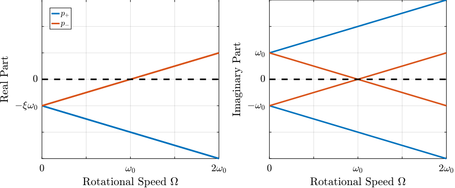

Campbell diagram - Real and Imaginary parts of the poles as a function of the rotating velocity

System Dynamics: Effect of rotation

The system dynamics from actuator forces $[F_u, F_v]$ to the relative motion $[d_u, d_v]$ is identified for several rotating velocities.

Looking at the transfer function matrix $\mathbf{G}_d$ in equation eqref:eq:Gd_w0_xi_k, one can see that the two diagonal (direct) terms are equal and that the two off-diagonal (coupling) terms are opposite. The bode plot of these two terms are shown in Figure ref:fig:rotating_direct_coupling_bode_plot for several rotational speeds $\Omega$. These plots confirm the expected behavior: the frequency of the two pairs of complex conjugate poles are further separated as $\Omega$ increases. For $\Omega > \omega_0$, the low frequency pair of complex conjugate poles $p_{-}$ becomes unstable.

%% Bode plot of the direct and coupling terms for several rotating velocities
freqs = logspace(-1, 1, 1000);

figure;
tiledlayout(3, 2, 'TileSpacing', 'Compact', 'Padding', 'None');

% Magnitude
ax1 = nexttile([2, 1]);
hold on;
for i = 1:length(Wzs)
    plot(freqs, abs(squeeze(freqresp(Gs{i}('du', 'Fu'), freqs, 'rad/s'))), '-', 'color', colors(i,:))
end
hold off;
set(gca, 'XScale', 'log'); set(gca, 'YScale', 'log');
set(gca, 'XTickLabel',[]); ylabel('Magnitude [m/N]');
title('Direct terms: $d_u/F_u$, $d_v/F_v$');
ylim([1e-2, 1e2]);
yticks([1e-2,1e-1,1,1e1,1e2])
yticklabels({'$0.01/k$', '$0.1/k$', '$1/k$', '$10/k$', '$100/k$'})

ax2 = nexttile([2, 1]);
hold on;
for i = 1:length(Wzs)
    plot(freqs, abs(squeeze(freqresp(Gs{i}('dv', 'Fu'), freqs, 'rad/s'))), '-', 'color', colors(i,:), ...
         'DisplayName', sprintf('$\\Omega = %.1f \\omega_0$', Wzs(i)))
end
hold off;
set(gca, 'XScale', 'log'); set(gca, 'YScale', 'log');
set(gca, 'XTickLabel',[]); set(gca, 'YTickLabel',[]);
title('Coupling Terms: $d_u/F_v$, $d_v/F_u$');
ldg = legend('location', 'northeast', 'FontSize', 8, 'NumColumns', 1);
ldg.ItemTokenSize = [10, 1];
ylim([1e-2, 1e2]);

ax3 = nexttile;
hold on;
for i = 1:length(Wzs)
    plot(freqs, 180/pi*angle(squeeze(freqresp(Gs{i}('du', 'Fu'), freqs, 'rad/s'))), '-', 'color', colors(i,:))
end
hold off;
set(gca, 'XScale', 'log'); set(gca, 'YScale', 'lin');
xlabel('Frequency [rad/s]'); ylabel('Phase [deg]');
yticks(-180:90:180);
ylim([-180 180]);
xticks([1e-1,1,1e1])
xticklabels({'$0.1 \omega_0$', '$\omega_0$', '$10 \omega_0$'})

ax4 = nexttile;
hold on;
for i = 1:length(Wzs)
    plot(freqs, 180/pi*angle(squeeze(freqresp(Gs{i}('dv', 'Fu'), freqs, 'rad/s'))), '-', 'color', colors(i,:));
end
hold off;
set(gca, 'XScale', 'log'); set(gca, 'YScale', 'lin');
xlabel('Frequency [rad/s]'); set(gca, 'YTickLabel',[]);
xticks([1e-1,1,1e1])
xticklabels({'$0.1 \omega_0$', '$\omega_0$', '$10 \omega_0$'})

linkaxes([ax1,ax2,ax3,ax4],'x');
xlim([freqs(1), freqs(end)]);

linkaxes([ax1,ax2],'y');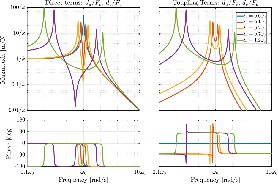

Bode plot of the direct and coupling terms for several rotating velocities

Integral Force Feedback

<<sec:rotating_iff_pure_int>>

Introduction   ignore

In order to further decrease the residual vibrations, active damping can be used for reducing the magnification of the response in the vicinity of the resonances cite:collette11_review_activ_vibrat_isolat_strat.

Many active damping techniques have been developed over the years such as Positive Position Feedback (PPF) cite:lin06_distur_atten_precis_hexap_point,fanson90_posit_posit_feedb_contr_large_space_struc, Integral Force Feedback (IFF) cite:preumont91_activ and Direct Velocity Feedback (DVF) cite:karnopp74_vibrat_contr_using_semi_activ_force_gener,serrand00_multic_feedb_contr_isolat_base_excit_vibrat,preumont02_force_feedb_versus_accel_feedb. \par

In cite:preumont92_activ_dampin_by_local_force, the IFF control scheme has been proposed, where a force sensor, a force actuator and an integral controller are used to directly augment the damping of a mechanical system. When the force sensor is collocated with the actuator, the open-loop transfer function has alternating poles and zeros which facilitate to guarantee the stability of the closed loop system cite:preumont02_force_feedb_versus_accel_feedb. It was latter shown that this property holds for multiple collated actuator/sensor pairs cite:preumont08_trans_zeros_struc_contr_with. \par

The main advantages of IFF over other active damping techniques are the guaranteed stability even in presence of flexible dynamics, good performances and robustness properties cite:preumont02_force_feedb_versus_accel_feedb. \par

Several improvements of the classical IFF have been proposed, such as adding a feed-through term to increase the achievable damping cite:teo15_optim_integ_force_feedb_activ_vibrat_contr or adding an high pass filter to recover the loss of compliance at low frequency cite:chesne16_enhan_dampin_flexib_struc_using_force_feedb. Recently, an $\mathcal{H}_\infty$ optimization criterion has been used to derive optimal gains for the IFF controller cite:zhao19_optim_integ_force_feedb_contr. \par

However, none of these study have been applied to a rotating system. In this section, Integral Force Feedback strategy is applied on the rotating suspended platform, and it is shown that gyroscopic effects alters the system dynamics and that IFF cannot be applied as is.

System and Equations of motion

In order to apply Integral Force Feedback, two force sensors are added in series with the actuators (Figure ref:fig:rotating_3dof_model_schematic_iff). Two identical controllers $K_F$ are then used to feedback each of the sensed force to its associated actuator:

\begin{equation} K_{F}(s) = g \cdot \frac{1}{s} \end{equation}

  \begin{tikzpicture}
    % Angle
    \def\thetau{25}

    % Rotational Stage
    \draw[fill=black!60!white] (0, 0) circle (4.3);
    \draw[fill=black!40!white] (0, 0) circle (3.8);

    % Label
    \node[anchor=north west, rotate=\thetau] at (-2.5, 2.5) {\small Rotating Stage};

    % Rotating Scope
    \begin{scope}[rotate=\thetau]
      % Rotating Frame
      \draw[fill=black!20!white] (-2.6, -2.6) rectangle (2.6, 2.6);
      % Label
      \node[anchor=north west, rotate=\thetau] at (-2.6, 2.6) {\small Suspended Platform};

      % Mass
      \draw[fill=white] (-1, -1) rectangle (1, 1);
      % Label
      \node[anchor=south west, rotate=\thetau] at (-1, -1) {\small Payload};

      % Attached Points
      \node[] at (-1, 0){$\bullet$};
      \draw[] (-1, 0) -- ++(-0.2, 0) coordinate(au);
      \node[] at (0, -1){$\bullet$};
      \draw[] (0, -1) -- ++(0, -0.2) coordinate(av);

      % Force Sensors
      \draw[draw=colorblue, fill=colorblue!10!white] ($(au) + (-0.2, -0.5)$) rectangle ($(au) + (0, 0.5)$);
      \draw[draw=colorblue] ($(au) + (-0.2, -0.5)$)coordinate(actu) -- ($(au) + (0,  0.5)$);
      \draw[draw=colorblue] ($(au) + (-0.2,  0.5)$)coordinate(ku)   -- ($(au) + (0, -0.5)$);

      \draw[draw=colorblue, fill=colorblue!10!white] ($(av) + (-0.5, -0.2)$) rectangle ($(av) + (0.5, 0)$);
      \draw[draw=colorblue] ($(av) + ( 0.5, -0.2)$)coordinate(actv) -- ($(av) + (-0.5,  0)$);
      \draw[draw=colorblue] ($(av) + (-0.5, -0.2)$)coordinate(kv)   -- ($(av) + ( 0.5,  0)$);

      % Spring and Actuator for U
      \draw[actuator={0.6}{0.2}{black}] (actu) -- coordinate[midway](actumid) (actu-|-2.6,0);
      \draw[spring=0.2] (ku) -- node[above=0.1, rotate=\thetau]{$k$} (ku-|-2.6,0);

      % \draw[actuator={0.6}{0.2}] (actv) -- node[right, rotate=\thetau]{$F_v$} (actv|-0,-2.6);
      \draw[actuator={0.6}{0.2}{black}] (actv) -- coordinate[midway](actvmid) (actv|-0,-2.6);
      \draw[spring=0.2] (kv) -- node[left, rotate=\thetau]{$k$} (kv|-0,-2.6);

      \node[color=colorblue, block={0.8cm}{0.6cm}, fill=colorblue!10!white, rotate=\thetau] (Ku) at ($(actumid) + (0, -1.2)$) {$K_{F}$};
      \draw[->, draw=colorblue] ($(au) + (-0.1, -0.5)$) |- (Ku.east) node[below right, rotate=\thetau]{$f_{u}$};
      \draw[->, draw=colorblue] (Ku.north) -- ($(actumid) + (0, -0.1)$) node[below left, rotate=\thetau]{$F_u$};

      \node[color=colorblue, block={0.8cm}{0.6cm}, fill=colorblue!10!white, rotate=\thetau] (Kv) at ($(actvmid) + (1.2, 0)$) {$K_{F}$};
      \draw[->, draw=colorblue] ($(av) + (0.5, -0.1)$) -| (Kv.north) node[above right, rotate=\thetau]{$f_{v}$};
      \draw[->, draw=colorblue] (Kv.west) -- ($(actvmid) + (0.1, 0)$) node[below right, rotate=\thetau]{$F_v$};
    \end{scope}

    % Inertial Frame
    \draw[->] (-4, -4) -- ++(2, 0) node[below]{$\vec{i}_x$};
    \draw[->] (-4, -4) -- ++(0, 2) node[left]{$\vec{i}_y$};
    \draw[fill, color=black] (-4, -4) circle (0.06);
    \node[draw, circle, inner sep=0pt, minimum size=0.3cm, label=left:$\vec{i}_z$] at (-4, -4){};

    \node[draw, circle, inner sep=0pt, minimum size=0.3cm] at (0, 0){};
    \draw[->] (0, 0) node[above left, rotate=\thetau]{$\vec{i}_w$} -- ++(\thetau:2) node[above, rotate=\thetau]{$\vec{i}_u$};
    \draw[->] (0, 0) -- ++(\thetau+90:2) node[left, rotate=\thetau]{$\vec{i}_v$};
    \draw[dashed] (0, 0) -- ++(2, 0);
    \draw[] (1.5, 0) arc (0:\thetau:1.5) node[midway, right]{$\theta$};
    \node[] at (0,0) {$\bullet$};

    \draw[->] (3.5, 0) arc (0:40:3.5) node[midway, left]{$\Omega$};
  \end{tikzpicture}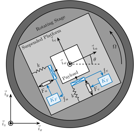

System with added Force Sensor in series with the actuators (shown in blue with the associated controllers)

The forces $\begin{bmatrix}f_u & f_v\end{bmatrix}$ measured by the two force sensors represented in Figure ref:fig:rotating_3dof_model_schematic_iff are described by equation eqref:eq:measured_force.

\begin{equation} \begin{bmatrix} f_{u} \\ f_{v} \end{bmatrix} = \begin{bmatrix} F_u \\ F_v \end{bmatrix} - (c s + k) \begin{bmatrix} d_u \\ d_v \end{bmatrix} \end{equation}

The transfer function matrix $\mathbf{G}_{f}$ from actuator forces to measured forces in equation eqref:eq:Gf_mimo_tf can be obtained by inserting equation eqref:eq:Gd_w0_xi_k into equation eqref:eq:measured_force. Its elements are shown in equation eqref:eq:Gf_indiv_el.

\begin{equation} \begin{bmatrix} f_{u} \\ f_{v} \end{bmatrix} = \mathbf{G}_{f} \begin{bmatrix} F_u \\ F_v \end{bmatrix} \end{equation} \begin{subequations} \label{eq:Gf} \begin{align} \mathbf{G}_{f}(1,1) &= \mathbf{G}_{f}(2,2) = \frac{\left( \frac{s^2}{{\omega_0}^2} - \frac{\Omega^2}{{\omega_0}^2} \right) \left( \frac{s^2}{{\omega_0}^2} + 2 \xi \frac{s}{\omega_0} + 1 - \frac{{\Omega}^2}{{\omega_0}^2} \right) + \left( 2 \frac{\Omega}{\omega_0} \frac{s}{\omega_0} \right)^2}{\left( \frac{s^2}{{\omega_0}^2} + 2 \xi \frac{s}{\omega_0} + 1 - \frac{{\Omega}^2}{{\omega_0}^2} \right)^2 + \left( 2 \frac{\Omega}{\omega_0} \frac{s}{\omega_0} \right)^2} \label{eq:Gf_diag_tf} \\ \mathbf{G}_{f}(1,2) &= -\mathbf{G}_{f}(2,1) = \frac{- \left( 2 \xi \frac{s}{\omega_0} + 1 \right) \left( 2 \frac{\Omega}{\omega_0} \frac{s}{\omega_0} \right)}{\left( \frac{s^2}{{\omega_0}^2} + 2 \xi \frac{s}{\omega_0} + 1 - \frac{{\Omega}^2}{{\omega_0}^2} \right)^2 + \left( 2 \frac{\Omega}{\omega_0} \frac{s}{\omega_0} \right)^2} \label{eq:Gf_off_diag_tf} \end{align} \end{subequations}

The zeros of the diagonal terms of $\mathbf{G}_f$ in equation eqref:eq:Gf_diag_tf are computed, and neglecting the damping for simplicity, two complex conjugated zeros $z_{c}$ are obtained in equation eqref:eq:iff_zero_cc, and two real zeros $z_{r}$ in equation eqref:eq:iff_zero_real.

\begin{subequations} \begin{align} z_c &= \pm j \omega_0 \sqrt{\frac{1}{2} \sqrt{8 \frac{\Omega^2}{{\omega_0}^2} + 1} + \frac{\Omega^2}{{\omega_0}^2} + \frac{1}{2} } \label{eq:iff_zero_cc} \\ z_r &= \pm \omega_0 \sqrt{\frac{1}{2} \sqrt{8 \frac{\Omega^2}{{\omega_0}^2} + 1} - \frac{\Omega^2}{{\omega_0}^2} - \frac{1}{2} } \label{eq:iff_zero_real} \end{align} \end{subequations}

It is interesting to see that the frequency of the pair of complex conjugate zeros $z_c$ in equation eqref:eq:iff_zero_cc always lies between the frequency of the two pairs of complex conjugate poles $p_{-}$ and $p_{+}$ in equation eqref:eq:pole_values. This is what usually gives the unconditional stability of IFF when collocated force sensors are used.

However, for non-null rotational speeds, the two real zeros $z_r$ in equation eqref:eq:iff_zero_real are inducing a non-minimum phase behavior. This can be seen in the Bode plot of the diagonal terms (Figure ref:fig:rotating_iff_bode_plot_effect_rot) where the low frequency gain is no longer zero while the phase stays at $\SI{180}{\degree}$.

The low frequency gain of $\mathbf{G}_f$ increases with the rotational speed $\Omega$ as shown in equation eqref:eq:low_freq_gain_iff_plan.

\begin{equation} \lim_{\omega \to 0} \left| \mathbf{G}_f (j\omega) \right| = \begin{bmatrix} \frac{\Omega^2}{{\omega_0}^2 - \Omega^2} & 0 \\ 0 & \frac{\Omega^2}{{\omega_0}^2 - \Omega^2} \end{bmatrix} \end{equation}

This can be explained as follows: a constant actuator force $F_u$ induces a small displacement of the mass $d_u = \frac{F_u}{k - m\Omega^2}$ (Hooke's law taking into account the negative stiffness induced by the rotation). This small displacement then increases the centrifugal force $m\Omega^2d_u = \frac{\Omega^2}{{\omega_0}^2 - \Omega^2} F_u$ which is then measured by the force sensors.

Effect of the rotation speed on the IFF plant dynamics

The transfer functions from actuator forces $[F_u,\ F_v]$ to the measured force sensors $[f_u,\ f_v]$ are identified for several rotating velocities and shown in Figure ref:fig:rotating_iff_bode_plot_effect_rot.

As was expected from the derived equations of motion:

• when $0 < \Omega < \omega_0$: the low frequency gain is no longer zero and two (non-minimum phase) real zero appears at low frequency. The low frequency gain increases with $\Omega$. A pair of (minimum phase) complex conjugate zeros appears between the two complex conjugate poles that are split further apart as $\Omega$ increases.
• when $\omega_0 < \Omega$: the low frequency pole becomes unstable.

%% Bode plot of the direct and coupling term for Integral Force Feedback - Effect of rotation
figure;
freqs = logspace(-2, 1, 1000);

figure;
tiledlayout(3, 2, 'TileSpacing', 'Compact', 'Padding', 'None');

% Magnitude
ax1 = nexttile([2, 1]);
hold on;
for i = 1:length(Wzs)
    plot(freqs, abs(squeeze(freqresp(Gs{i}('fu', 'Fu'), freqs, 'rad/s'))), '-', 'color', colors(i,:))
end
hold off;
set(gca, 'XScale', 'log'); set(gca, 'YScale', 'log');
set(gca, 'XTickLabel',[]); ylabel('Magnitude [N/N]');
title('Direct terms: $f_u/F_u$, $f_v/F_v$');
ylim([1e-3, 1e2]);

ax2 = nexttile([2, 1]);
hold on;
for i = 1:length(Wzs)
    plot(freqs, abs(squeeze(freqresp(Gs{i}('fv', 'Fu'), freqs, 'rad/s'))), '-', 'color', colors(i,:), ...
         'DisplayName', sprintf('$\\Omega = %.1f \\omega_0$', Wzs(i)))
end
hold off;
set(gca, 'XScale', 'log'); set(gca, 'YScale', 'log');
set(gca, 'XTickLabel',[]); set(gca, 'YTickLabel',[]);
title('Coupling Terms: $f_u/F_v$, $f_v/F_u$');
ldg = legend('location', 'northwest', 'FontSize', 8, 'NumColumns', 1);
ldg.ItemTokenSize = [10, 1];
ylim([1e-3, 1e2]);

ax3 = nexttile;
hold on;
for i = 1:length(Wzs)
    plot(freqs, 180/pi*angle(squeeze(freqresp(Gs{i}('fu', 'Fu'), freqs, 'rad/s'))), '-', 'color', colors(i,:))
end
hold off;
set(gca, 'XScale', 'log'); set(gca, 'YScale', 'lin');
xlabel('Frequency [rad/s]'); ylabel('Phase [deg]');
yticks(-180:90:180);
ylim([-180 180]);
xticks([1e-2,1e-1,1,1e1])
xticklabels({'$0.01 \omega_0$', '$0.1 \omega_0$', '$\omega_0$', '$10 \omega_0$'})

ax4 = nexttile;
hold on;
for i = 1:length(Wzs)
    plot(freqs, 180/pi*angle(squeeze(freqresp(Gs{i}('fv', 'Fu'), freqs, 'rad/s'))), '-', 'color', colors(i,:));
end
hold off;
set(gca, 'XScale', 'log'); set(gca, 'YScale', 'lin');
xlabel('Frequency [rad/s]'); set(gca, 'YTickLabel',[]);
yticks(-180:90:180);
ylim([-180 180]);
xticks([1e-2,1e-1,1,1e1])
xticklabels({'$0.01 \omega_0$', '$0.1 \omega_0$', '$\omega_0$', '$10 \omega_0$'})

linkaxes([ax1,ax2,ax3,ax4],'x');
xlim([freqs(1), freqs(end)]);

linkaxes([ax1,ax2],'y');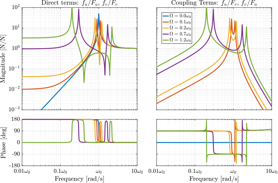

Bode plot of the direct and coupling term for Integral Force Feedback - Effect of rotation

Decentralized Integral Force Feedback

The control diagram for decentralized Integral Force Feedback is shown in Figure ref:fig:rotating_iff_diagram.

\tikzset{block/.default={0.8cm}{0.8cm}}
\tikzset{addb/.append style={scale=0.7}}
\tikzset{node distance=0.6}

\begin{tikzpicture}
  \node[block={1.8cm}{2.2cm}] (G) {$\bm{G}_f$};

  % Inputs of the controllers
  \coordinate[] (output1) at ($(G.south east)!0.75!(G.north east)$);
  \coordinate[] (output2) at ($(G.south east)!0.25!(G.north east)$);
  \coordinate[] (input1)  at ($(G.south west)!0.75!(G.north west)$);
  \coordinate[] (input2)  at ($(G.south west)!0.25!(G.north west)$);

  \node[block, left=1.8 of input1] (K1) {$g/s$};
  \node[block] (K2) at ($(K1.east|-input2)+(0.6, 0)$) {$g/s$};

  % Connections and labels
  \draw[->] (K1.east) -- (input1)node[above left]{$F_u$};
  \draw[->] (K2.east) -- (input2)node[above left]{$F_v$};

  \draw[->] (output1) -- ++(0.8, 0) node[above left]{$f_u$};
  \draw[->] (output2) -- ++(0.8, 0) node[above left]{$f_v$};

  \draw[->] ($(output1)+(0.2, 0)$)node[branch]{} -- ++(0,  1.2) -| ($(K1.west) + (-0.8, 0)$)coordinate(start) -- (K1.west);
  \draw[->] ($(output2)+(0.2, 0)$)node[branch]{} -- ++(0, -1.2) -| (start|-K2) -- (K2.west);

  \begin{scope}[on background layer]
    \node[fit={(K1.north west) (K2.south east)}, inner sep=6pt, draw, dashed, fill=black!20!white] (K) {};
    \node[below left] at (K.north east) {$\bm{K}_F$};
  \end{scope}
\end{tikzpicture}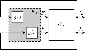

Control diagram for decentralized Integral Force Feedback

The decentralized IFF controller $\bm{K}_F$ corresponds to a diagonal controller with integrators:

\begin{equation} \begin{aligned} \mathbf{K}_{F}(s) &= \begin{bmatrix} K_{F}(s) & 0 \\ 0 & K_{F}(s) \end{bmatrix} \\ K_{F}(s) &= g \cdot \frac{1}{s} \end{aligned} \end{equation}

In order to see how the IFF controller affects the poles of the closed loop system, a Root Locus plot (Figure ref:fig:rotating_root_locus_iff_pure_int) is constructed as follows: the poles of the closed-loop system are drawn in the complex plane as the controller gain $g$ varies from $0$ to $\infty$ for the two controllers $K_{F}$ simultaneously. As explained in cite:preumont08_trans_zeros_struc_contr_with,skogestad07_multiv_feedb_contr, the closed-loop poles start at the open-loop poles (shown by $\tikz[baseline=-0.6ex] \node[cross out, draw=black, minimum size=1ex, line width=2pt, inner sep=0pt, outer sep=0pt] at (0, 0){};$) for $g = 0$ and coincide with the transmission zeros (shown by $\tikz[baseline=-0.6ex] \draw[line width=2pt, inner sep=0pt, outer sep=0pt] (0,0) circle[radius=3pt];$) as $g \to \infty$.

Whereas collocated IFF is usually associated with unconditional stability cite:preumont91_activ, this property is lost due to gyroscopic effects as soon as the rotation velocity in non-null. This can be seen in the Root Locus plot (Figure ref:fig:rotating_root_locus_iff_pure_int) where poles corresponding to the controller are bound to the right half plane implying closed-loop system instability.

Physically, this can be explained like so: at low frequency, the loop gain is very large due to the pure integrator in $K_{F}$ and the finite gain of the plant (Figure ref:fig:rotating_iff_bode_plot_effect_rot). The control system is thus canceling the spring forces which makes the suspended platform no able to hold the payload against centrifugal forces, hence the instability.

%% Root Locus for the Decentralized Integral Force Feedback controller
figure;

Kiff = 1/s*eye(2);

gains = logspace(-2, 4, 300);
Wz_i = [1,3,4];

hold on;
for i = 1:length(Wz_i)
    plot(real(pole(Gs{Wz_i(i)}({'fu', 'fv'}, {'Fu', 'Fv'})*Kiff)),  imag(pole(Gs{Wz_i(i)}({'fu', 'fv'}, {'Fu', 'Fv'})*Kiff)), 'x', 'color', colors(i,:), ...
         'DisplayName', sprintf('$\\Omega = %.1f \\omega_0 $', Wzs(Wz_i(i))),'MarkerSize',8);
    plot(real(tzero(Gs{Wz_i(i)}({'fu', 'fv'}, {'Fu', 'Fv'})*Kiff)),  imag(tzero(Gs{Wz_i(i)}({'fu', 'fv'}, {'Fu', 'Fv'})*Kiff)), 'o', 'color', colors(i,:), ...
         'HandleVisibility', 'off','MarkerSize',8);
    for g = gains
        cl_poles = pole(feedback(Gs{Wz_i(i)}({'fu', 'fv'}, {'Fu', 'Fv'}), g*Kiff, -1));
        plot(real(cl_poles), imag(cl_poles), '.', 'color', colors(i,:), ...
             'HandleVisibility', 'off','MarkerSize',4);
    end
end
hold off;
axis square;
xlim([-1.8, 0.2]); ylim([0, 2]);
xticks([-1, 0])
xticklabels({'-$\omega_0$', '$0$'})
yticks([0, 1, 2])
yticklabels({'$0$', '$\omega_0$', '$2 \omega_0$'})

xlabel('Real Part'); ylabel('Imaginary Part');
leg = legend('location', 'northwest', 'FontSize', 8);
leg.ItemTokenSize(1) = 8;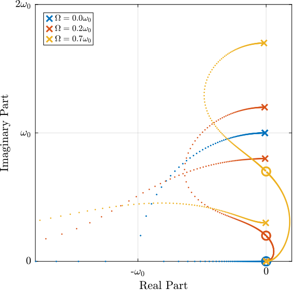

Root Locus for the Decentralized Integral Force Feedback controller. Several rotating speed are shown.

Integral Force Feedback with an High Pass Filter

<<sec:rotating_iff_pseudo_int>>

Introduction   ignore

As was explained in the previous section, the instability of the IFF controller applied on the rotating system comes in part from the high gain at low frequency caused by the pure integrators.

In order to limit the low frequency controller gain, an High Pass Filter (HPF) can be added to the controller as shown in equation eqref:eq:iff_lhf.

\begin{equation} \boxed{K_{F}(s) = g \cdot \frac{1}{s} \cdot \underbrace{\frac{s/\omega_i}{1 + s/\omega_i}}_{\text{HPF}} = g \cdot \frac{1}{s + \omega_i}} \end{equation}

This is equivalent as to slightly shifting the controller pole to the left along the real axis.

This modification of the IFF controller is typically done to avoid saturation associated with the pure integrator cite:preumont91_activ,marneffe07_activ_passiv_vibrat_isolat_dampin_shunt_trans. This is however not why this high pass filter is added here.

Modified Integral Force Feedback Controller

The Integral Force Feedback Controller is modified such that instead of using pure integrators, pseudo integrators (i.e. low pass filters) are used:

\begin{equation} K_{\text{IFF}}(s) = g\frac{1}{\omega_i + s} \begin{bmatrix} 1 & 0 \\ 0 & 1 \end{bmatrix} \end{equation}

where $\omega_i$ characterize down to which frequency the signal is integrated.

Let's arbitrary choose the following control parameters:

%% Modified IFF - parameters
g = 2; % Controller gain
wi = 0.1; % HPF Cut-Off frequency [rad/s]

Kiff     = (g/s)*eye(2); % Pure IFF
Kiff_hpf = (g/(wi+s))*eye(2); % IFF with added HPF

The loop gains ($K_F(s)$ times the direct dynamics $f_u/F_u$) with and without the added HPF are shown in Figure ref:fig:rotating_iff_modified_loop_gain. The effect of the added HPF limits the low frequency gain to finite values as expected.

%% Loop gain for the IFF with pure integrator and modified IFF with added high pass filter
freqs = logspace(-2, 1, 1000);
Wz_i = 2;

figure;
tiledlayout(3, 1, 'TileSpacing', 'Compact', 'Padding', 'None');

% Magnitude
ax1 = nexttile([2, 1]);
hold on;
plot(freqs, abs(squeeze(freqresp(Gs{Wz_i}('fu', 'Fu')*Kiff(1,1), freqs, 'rad/s'))))
plot(freqs, abs(squeeze(freqresp(Gs{Wz_i}('fu', 'Fu')*Kiff_hpf(1,1), freqs, 'rad/s'))))
hold off;
set(gca, 'XScale', 'log'); set(gca, 'YScale', 'log');
set(gca, 'XTickLabel',[]); ylabel('Loop Gain');

% Phase
ax2 = nexttile;
hold on;
plot(freqs, 180/pi*angle(squeeze(freqresp(Gs{Wz_i}('fu', 'Fu')*Kiff(1,1), freqs, 'rad/s'))), 'DisplayName', 'IFF')
plot(freqs, 180/pi*angle(squeeze(freqresp(Gs{Wz_i}('fu', 'Fu')*Kiff_hpf(1,1), freqs, 'rad/s'))), 'DisplayName', 'IFF + HPF')
hold off;
set(gca, 'XScale', 'log'); set(gca, 'YScale', 'lin');
xlabel('Frequency [rad/s]'); ylabel('Phase [deg]');
yticks(-180:90:180);
ylim([-180 180]);
xticks([1e-2,1e-1,1,1e1])
xticklabels({'$0.01 \omega_0$', '$0.1 \omega_0$', '$\omega_0$', '$10 \omega_0$'})
leg = legend('location', 'southwest', 'FontSize', 8);
leg.ItemTokenSize(1) = 20;

linkaxes([ax1,ax2],'x');
xlim([freqs(1), freqs(end)]);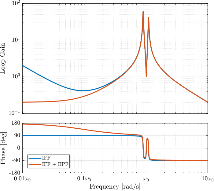

Loop gain for the IFF with pure integrator and modified IFF with added high pass filter ($\Omega = 0.1\omega_0$)

The Root Locus plots for the decentralized IFF with and without the HPF are displayed in Figure ref:fig:rotating_iff_root_locus_hpf. With the added HPF, the poles of the closed loop system are shown to be stable up to some value of the gain $g_\text{max}$ given by equation eqref:eq:gmax_iff_hpf.

\begin{equation} \boxed{g_{\text{max}} = \omega_i \left( \frac{{\omega_0}^2}{\Omega^2} - 1 \right)} \end{equation}

It is interesting to note that $g_{\text{max}}$ also corresponds to the controller gain at which the low frequency loop gain (Figure ref:fig:rotating_iff_modified_loop_gain) reaches one.

%% Root Locus for the initial IFF and the modified IFF
gains = logspace(-2, 4, 200);

figure;
tiledlayout(1, 3, 'TileSpacing', 'Compact', 'Padding', 'None');

ax1 = nexttile([1,2]);
hold on;
for g = gains
    clpoles = pole(feedback(Gs{Wz_i}({'fu', 'fv'}, {'Fu', 'Fv'}), g*Kiff));
    plot(real(clpoles), imag(clpoles), '.', 'color', colors(1,:), 'HandleVisibility', 'off','MarkerSize',4);
end
for g = gains
    clpoles = pole(feedback(Gs{Wz_i}({'fu', 'fv'}, {'Fu', 'Fv'}), g*Kiff_hpf));
    plot(real(clpoles), imag(clpoles), '.', 'color', colors(2,:), 'HandleVisibility', 'off','MarkerSize',4);
end
% Pure Integrator
plot(real(pole(Gs{Wz_i}({'fu', 'fv'}, {'Fu', 'Fv'})*Kiff)), ...
     imag(pole(Gs{Wz_i}({'fu', 'fv'}, {'Fu', 'Fv'})*Kiff)), ...
     'x', 'color', colors(1,:), 'DisplayName', 'IFF','MarkerSize',8);
plot(real(tzero(Gs{Wz_i}({'fu', 'fv'}, {'Fu', 'Fv'})*Kiff)), ...
     imag(tzero(Gs{Wz_i}({'fu', 'fv'}, {'Fu', 'Fv'})*Kiff)), ...
     'o', 'color', colors(1,:), 'HandleVisibility', 'off','MarkerSize',8);
% Modified IFF
plot(real(pole(Gs{Wz_i}({'fu', 'fv'}, {'Fu', 'Fv'})*Kiff_hpf)), ...
     imag(pole(Gs{Wz_i}({'fu', 'fv'}, {'Fu', 'Fv'})*Kiff_hpf)), ...
     'x', 'color', colors(2,:), 'DisplayName', 'IFF + HPF','MarkerSize',8);
plot(real(tzero(Gs{Wz_i}({'fu', 'fv'}, {'Fu', 'Fv'})*Kiff_hpf)), ...
     imag(tzero(Gs{Wz_i}({'fu', 'fv'}, {'Fu', 'Fv'})*Kiff_hpf)), ...
     'o', 'color', colors(2,:), 'HandleVisibility', 'off','MarkerSize',8);
hold off;
axis square;
leg = legend('location', 'northwest', 'FontSize', 8);
leg.ItemTokenSize(1) = 8;
xlabel('Real Part'); ylabel('Imaginary Part');

xlim([-2.25, 0.25]); ylim([-1.25, 1.25]);
xticks([-2, -1, 0])
xticklabels({'$-2\omega_0$', '$-\omega_0$', '$0$'})
yticks([-1, 0, 1])
yticklabels({'$-\omega_0$', '$0$', '$\omega_0$'})

ax2 = nexttile();
hold on;
for g = gains
    clpoles = pole(feedback(Gs{Wz_i}({'fu', 'fv'}, {'Fu', 'Fv'}), g*Kiff));
    plot(real(clpoles), imag(clpoles), '.', 'color', colors(1,:),'MarkerSize',4);
end
for g = gains
    clpoles = pole(feedback(Gs{Wz_i}({'fu', 'fv'}, {'Fu', 'Fv'}), g*Kiff_hpf));
    plot(real(clpoles), imag(clpoles), '.', 'color', colors(2,:),'MarkerSize',4);
end
% Pure Integrator
plot(real(pole(Gs{Wz_i}({'fu', 'fv'}, {'Fu', 'Fv'})*Kiff)), ...
     imag(pole(Gs{Wz_i}({'fu', 'fv'}, {'Fu', 'Fv'})*Kiff)), ...
     'x', 'color', colors(1,:),'MarkerSize',8);
plot(real(tzero(Gs{Wz_i}({'fu', 'fv'}, {'Fu', 'Fv'})*Kiff)), ...
     imag(tzero(Gs{Wz_i}({'fu', 'fv'}, {'Fu', 'Fv'})*Kiff)), ...
     'o', 'color', colors(1,:),'MarkerSize',8);
% Modified IFF
plot(real(pole(Gs{Wz_i}({'fu', 'fv'}, {'Fu', 'Fv'})*Kiff_hpf)), ...
     imag(pole(Gs{Wz_i}({'fu', 'fv'}, {'Fu', 'Fv'})*Kiff_hpf)), ...
     'x', 'color', colors(2,:),'MarkerSize',8);
plot(real(tzero(Gs{Wz_i}({'fu', 'fv'}, {'Fu', 'Fv'})*Kiff_hpf)), ...
     imag(tzero(Gs{Wz_i}({'fu', 'fv'}, {'Fu', 'Fv'})*Kiff_hpf)), ...
     'o', 'color', colors(2,:),'MarkerSize',8);
hold off;
axis square;
xlabel('Real Part'); ylabel('Imaginary Part');
title('Zoom near the origin');

xlim([-0.15, 0.1]); ylim([-0.15, 0.15]);
xticks([-0.1, 0, 0.1])
xticklabels({'$-0.1\omega_0$', '$0$', '$0.1\omega_0$'})
yticks([-0.1, 0, 0.1])
yticklabels({'$-0.1\omega_0$', '$0$', '$0.1\omega_0$'})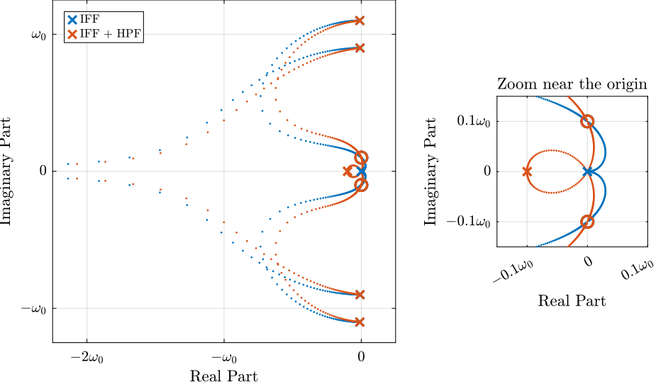

Root Locus for the initial IFF and the modified IFF

Optimal IFF with HPF parameters $\omega_i$ and $g$

Two parameters can be tuned for the modified controller in equation eqref:eq:iff_lhf: the gain $g$ and the pole's location $\omega_i$. The optimal values of $\omega_i$ and $g$ are here considered as the values for which the damping of all the closed-loop poles are simultaneously maximized.

In order to visualize how $\omega_i$ does affect the attainable damping, the Root Locus plots for several $\omega_i$ are displayed in Figure ref:fig:rotating_root_locus_iff_modified_effect_wi. It is shown that even though small $\omega_i$ seem to allow more damping to be added to the suspension modes, the control gain $g$ may be limited to small values due to equation eqref:eq:gmax_iff_hpf.

%% High Pass Filter Cut-Off Frequency
wis = [0.01, 0.1, 0.5, 1]*Wzs(2); % [rad/s]

%% Root Locus for the initial IFF and the modified IFF
gains = logspace(-2, 4, 200);

figure;
tiledlayout(1, 2, 'TileSpacing', 'Compact', 'Padding', 'None');

ax1 = nexttile();
hold on;
for wi_i = 1:length(wis)
    wi = wis(wi_i);
    Kiff = (1/(wi+s))*eye(2);
    L(wi_i) = plot(nan, nan, '.', 'color', colors(wi_i,:), 'DisplayName', sprintf('$\\omega_i = %.2f \\omega_0$', wi./Wzs(2)));
    for g = gains
        clpoles = pole(feedback(Gs{2}({'fu', 'fv'}, {'Fu', 'Fv'}), g*Kiff));
        plot(real(clpoles), imag(clpoles), '.', 'color', colors(wi_i,:),'MarkerSize',4);
    end
    plot(real(pole(Gs{2}({'fu', 'fv'}, {'Fu', 'Fv'})*Kiff)), ...
         imag(pole(Gs{2}({'fu', 'fv'}, {'Fu', 'Fv'})*Kiff)), ...
         'x', 'color', colors(wi_i,:),'MarkerSize',8);
    plot(real(tzero(Gs{2}({'fu', 'fv'}, {'Fu', 'Fv'})*Kiff)), ...
         imag(tzero(Gs{2}({'fu', 'fv'}, {'Fu', 'Fv'})*Kiff)), ...
         'o', 'color', colors(wi_i,:),'MarkerSize',8);
end
hold off;
axis square;
xlim([-2.3, 0.1]); ylim([-1.2, 1.2]);
xticks([-2:1:2]); yticks([-2:1:2]);
leg = legend(L, 'location', 'northwest', 'FontSize', 8);
leg.ItemTokenSize(1) = 8;
xlabel('Real Part'); ylabel('Imaginary Part');
clear L

xlim([-2.25, 0.25]); ylim([-1.25, 1.25]);
xticks([-2, -1, 0])
xticklabels({'$-2\omega_0$', '$-\omega_0$', '$0$'})
yticks([-1, 0, 1])
yticklabels({'$-\omega_0$', '$0$', '$\omega_0$'})

ax2 = nexttile();
hold on;
for wi_i = 1:length(wis)
    wi = wis(wi_i);
    Kiff = (1/(wi+s))*eye(2);
    L(wi_i) = plot(nan, nan, '.', 'color', colors(wi_i,:));
    for g = gains
        clpoles = pole(feedback(Gs{2}({'fu', 'fv'}, {'Fu', 'Fv'}), g*Kiff));
        plot(real(clpoles), imag(clpoles), '.', 'color', colors(wi_i,:),'MarkerSize',4);
    end
    plot(real(pole(Gs{2}({'fu', 'fv'}, {'Fu', 'Fv'})*Kiff)), ...
         imag(pole(Gs{2}({'fu', 'fv'}, {'Fu', 'Fv'})*Kiff)), ...
         'x', 'color', colors(wi_i,:),'MarkerSize',8);
    plot(real(tzero(Gs{2}({'fu', 'fv'}, {'Fu', 'Fv'})*Kiff)), ...
         imag(tzero(Gs{2}({'fu', 'fv'}, {'Fu', 'Fv'})*Kiff)), ...
         'o', 'color', colors(wi_i,:),'MarkerSize',8);
end
hold off;
axis square;
xlim([-2.3, 0.1]); ylim([-1.2, 1.2]);
xticks([-2:1:2]); yticks([-2:1:2]);
xlabel('Real Part'); ylabel('Imaginary Part');
title('Zoom near the origin');
clear L

xlim([-0.15, 0.1]); ylim([-0.15, 0.15]);
xticks([-0.1, 0, 0.1])
xticklabels({'$-0.1\omega_0$', '$0$', '$0.1\omega_0$'})
yticks([-0.1, 0, 0.1])
yticklabels({'$-0.1\omega_0$', '$0$', '$0.1\omega_0$'})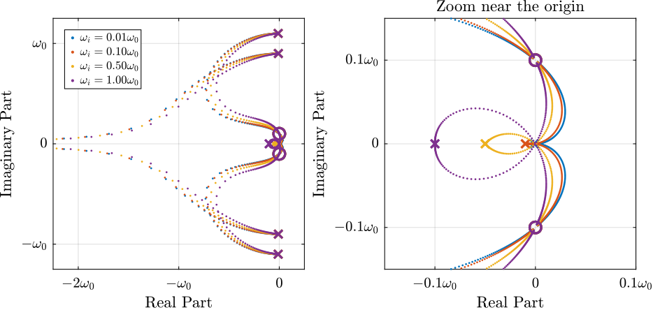

Root Locus for several high pass filter cut-off frequency

In order to study this trade off, the attainable closed-loop damping ratio $\xi_{\text{cl}}$ is computed as a function of $\omega_i/\omega_0$. The gain $g_{\text{opt}}$ at which this maximum damping is obtained is also displayed and compared with the gain $g_{\text{max}}$ at which the system becomes unstable (Figure ref:fig:rotating_iff_hpf_optimal_gain).

Three regions can be observed:

• $\omega_i/\omega_0 < 0.02$: the added damping is limited by the maximum allowed control gain $g_{\text{max}}$
• $0.02 < \omega_i/\omega_0 < 0.2$: the attainable damping ratio is maximized and is reached for $g \approx 2$
• $0.2 < \omega_i/\omega_0$: the added damping decreases as $\omega_i/\omega_0$ increases.

%% Compute the optimal control gain
wis = logspace(-2, 1, 100); % [rad/s]

opt_xi = zeros(1, length(wis)); % Optimal simultaneous damping
opt_gain = zeros(1, length(wis)); % Corresponding optimal gain

for wi_i = 1:length(wis)
    wi = wis(wi_i);
    Kiff = 1/(s + wi)*eye(2);

    fun = @(g)computeSimultaneousDamping(g, Gs{2}({'fu', 'fv'}, {'Fu', 'Fv'}), Kiff);

    [g_opt, xi_opt] = fminsearch(fun, 0.5*wi*((1/Wzs(2))^2 - 1));
    opt_xi(wi_i) = 1/xi_opt;
    opt_gain(wi_i) = g_opt;
end

%% Attainable damping ratio as a function of wi/w0. Corresponding control gain g_opt and g_max are also shown
figure;
yyaxis left
plot(wis, opt_xi, '-', 'DisplayName', '$\xi_{cl}$');
set(gca, 'YScale', 'lin');
ylim([0,1]);
ylabel('Damping Ratio $\xi$');

yyaxis right
hold on;
plot(wis, opt_gain, '-', 'DisplayName', '$g_{opt}$');
plot(wis, wis*((1/Wzs(2))^2 - 1), '--', 'DisplayName', '$g_{max}$');
set(gca, 'YScale', 'lin');
ylim([0,10]);
ylabel('Controller gain $g$');

xlabel('$\omega_i/\omega_0$');
set(gca, 'XScale', 'log');
legend('location', 'northeast', 'FontSize', 8);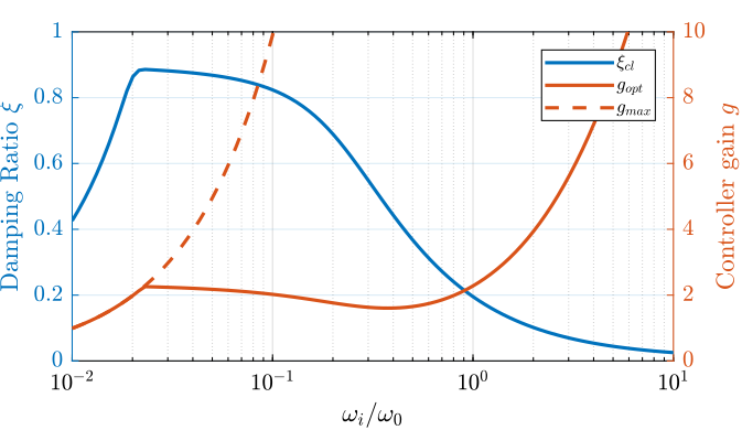

Attainable damping ratio $\xi_\text{cl}$ as a function of $\omega_i/\omega_0$. Corresponding control gain $g_\text{opt}$ and $g_\text{max}$ are also shown

Obtained Damped Plant

Let's choose $\omega_i = 0.1 \cdot \omega_0$ and compute the damped plant. The undamped and damped plants are compared in Figure ref:fig:rotating_iff_hpf_damped_plant in blue and red respectively. A well damped plant is indeed obtained.

However, the magnitude of the coupling term ($d_v/F_u$) is larger then IFF is applied.

%% Compute damped plant
wi = 0.1; % [rad/s]
g = 2; % Gain
Kiff_hpf = (g/(wi+s))*eye(2); % IFF with added HPF
Kiff_hpf.InputName = {'fu', 'fv'};
Kiff_hpf.OutputName = {'Fu', 'Fv'};

G_iff_hpf = feedback(Gs{2}, Kiff_hpf, 'name');

isstable(G_iff_hpf) % Verify stability

%% Damped plant with IFF and added HPF - Transfer function from $F_u$ to $d_u$
freqs = logspace(-2, 1, 1000);

figure;
tiledlayout(3, 1, 'TileSpacing', 'Compact', 'Padding', 'None');

% Magnitude
ax1 = nexttile([2, 1]);
hold on;
plot(freqs, abs(squeeze(freqresp(Gs{2}('Du', 'Fu'), freqs, 'rad/s'))), '-', 'color', [zeros(1,3)], ...
    'DisplayName', '$d_u/F_u$, OL')
plot(freqs, abs(squeeze(freqresp(G_iff_hpf('Du', 'Fu'), freqs, 'rad/s'))), '-', 'color', [colors(1,:)], ...
    'DisplayName', '$d_u/F_u$, IFF')
plot(freqs, abs(squeeze(freqresp(Gs{2}('Dv', 'Fu'), freqs, 'rad/s'))), '-', 'color', [zeros(1,3), 0.5], ...
    'DisplayName', '$d_v/F_u$, OL')
plot(freqs, abs(squeeze(freqresp(G_iff_hpf('Dv', 'Fu'), freqs, 'rad/s'))), '-', 'color', [colors(1,:), 0.5], ...
    'DisplayName', '$d_v/F_u$, IFF')
hold off;
set(gca, 'XScale', 'log'); set(gca, 'YScale', 'log');
set(gca, 'XTickLabel',[]); ylabel('Magnitude [m/N]');
leg = legend('location', 'southwest', 'FontSize', 8, 'NumColumns', 2);
leg.ItemTokenSize(1) = 20;

ax2 = nexttile;
hold on;
plot(freqs, 180/pi*angle(squeeze(freqresp(Gs{2}('Du', 'Fu'), freqs, 'rad/s'))), '-', 'color', zeros(1,3))
plot(freqs, 180/pi*angle(squeeze(freqresp(G_iff_hpf('Du', 'Fu'), freqs, 'rad/s'))), '-', 'color', colors(1,:))
hold off;
set(gca, 'XScale', 'log'); set(gca, 'YScale', 'lin');
xlabel('Frequency [rad/s]'); ylabel('Phase [deg]');
yticks(-180:90:180);
ylim([-180 180]);
xticks([1e-2,1e-1,1,1e1])
xticklabels({'$0.01 \omega_0$', '$0.1 \omega_0$', '$\omega_0$', '$10 \omega_0$'})

linkaxes([ax1,ax2],'x');
xlim([freqs(1), freqs(end)]);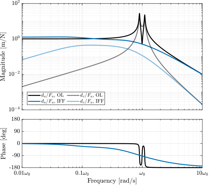

Damped plant with IFF and added HPF - Transfer function from $F_u$ to $d_u$, $\omega_i = 0.1 \cdot \omega_0$, $\Omega = 0.1 \cdot \omega_0$

In order to study how $\omega_i$ affects the coupling of the damped plant, the closed-loop plant is identified for several $\omega_i$. The direct and coupling terms of the plants are shown in Figure ref:fig:rotating_iff_hpf_damped_plant_effect_wi_coupling (left) and the ratio between the two (i.e. the coupling ratio) is shown in Figure ref:fig:rotating_iff_hpf_damped_plant_effect_wi_coupling (right).

The coupling ratio is decreasing as $\omega_i$ increases. There is therefore a trade-off between achievable damping and coupling ratio for the choice of $\omega_i$. The same trade-off can be seen between achievable damping and loss of compliance at low frequency (see Figure ref:fig:rotating_iff_hpf_effect_wi_compliance).

%% Compute damped plant
wis = [0.03, 0.1, 0.5]; % [rad/s]
g = 2; % Gain

Gs_iff_hpf  = {};

for i = 1:length(wis)
    Kiff_hpf = (g/(wis(i)+s))*eye(2); % IFF with added HPF
    Kiff_hpf.InputName = {'fu', 'fv'};
    Kiff_hpf.OutputName = {'Fu', 'Fv'};

    Gs_iff_hpf(i) = {feedback(Gs{2}, Kiff_hpf, 'name')};
end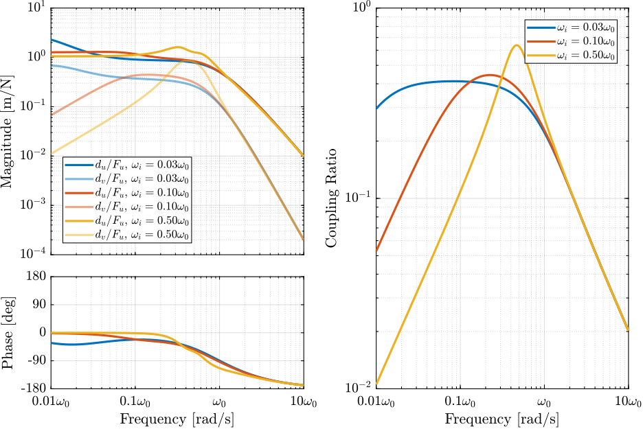

Effect of $\omega_i$ on the damped plant coupling

Effect of $\omega_i$ on the obtained compliance

IFF with a stiffness in parallel with the force sensor

<<sec:rotating_iff_parallel_stiffness>>

Introduction   ignore

In this section it is proposed to add springs in parallel with the force sensors to counteract the negative stiffness induced by the gyroscopic effects.

Such springs are schematically shown in Figure ref:fig:rotating_3dof_model_schematic_iff_parallel_springs where $k_a$ is the stiffness of the actuator and $k_p$ the added stiffness in parallel with the actuator and force sensor.

\begin{tikzpicture}
  % Angle
  \def\thetau{25}

  % Rotational Stage
  \draw[fill=black!60!white] (0, 0) circle (4.3);
  \draw[fill=black!40!white] (0, 0) circle (3.8);

  % Label
  \node[anchor=north west, rotate=\thetau] at (-2.5, 2.5) {\small Rotating Stage};

  % Rotating Scope
  \begin{scope}[rotate=\thetau]
    % Rotating Frame
    \draw[fill=black!20!white] (-2.6, -2.6) rectangle (2.6, 2.6);
    % Label
    \node[anchor=north west, rotate=\thetau] at (-2.6, 2.6) {\small Suspended Platform};

    % Mass
    \draw[fill=white] (-1, -1) rectangle (1, 1);
    % Label
    \node[anchor=south west, rotate=\thetau] at (-1, -1) {\small Payload};

    % Attached Points
    \draw[] (-1, 0) -- ++(-0.2, 0) coordinate(au);
    \draw[] (0, -1) -- ++(0, -0.2) coordinate(av);

    % Force Sensors
    \draw[fill=white] ($(au) + (-0.2, -0.5)$) rectangle ($(au) + (0, 0.5)$);
    \draw[] ($(au) + (-0.2, -0.5)$)coordinate(actu) -- ($(au) + (0,  0.5)$);
    \draw[] ($(au) + (-0.2,  0.5)$)coordinate(ku)   -- ($(au) + (0, -0.5)$);
    \node[below=0.1, rotate=\thetau] at ($(au) + (-0.1, -0.5)$) {$f_{u}$};

    \draw[fill=white] ($(av) + (-0.5, -0.2)$) rectangle ($(av) + (0.5, 0)$);
    \draw[] ($(av) + ( 0.5, -0.2)$)coordinate(actv) -- ($(av) + (-0.5,  0)$);
    \draw[] ($(av) + (-0.5, -0.2)$)coordinate(kv)   -- ($(av) + ( 0.5,  0)$);
    \node[right=0.1, rotate=\thetau] at ($(av) + (0.5, -0.1)$) {$f_{v}$};

    % Spring and Actuator for U
    \draw[actuator={0.6}{0.2}{black}] (actu) -- node[below=0.1, rotate=\thetau]{$F_u$} (actu-|-2.6,0);
    \draw[spring=0.2] (ku) -- node[below=0.1, rotate=\thetau]{$k_a$} (ku-|-2.6,0);
    \draw[spring=0.2,draw=colorred] (-1, 0.8) -- node[above=0.1, rotate=\thetau, color=colorred]{$k_p$} (-1, 0.8-|-2.6,0);

    \draw[actuator={0.6}{0.2}{black}] (actv) -- node[right=0.1, rotate=\thetau]{$F_v$} (actv|-0,-2.6);
    \draw[spring=0.2] (kv) -- node[right=0.1, rotate=\thetau]{$k_a$} (kv|-0,-2.6);
    \draw[spring=0.2, draw=colorred] (-0.8, -1) -- node[left=0.1, rotate=\thetau, color=colorred]{$k_p$} (-0.8, -1|-0,-2.6);
  \end{scope}

  % Inertial Frame
  \draw[->] (-4, -4) -- ++(2, 0) node[below]{$\vec{i}_x$};
  \draw[->] (-4, -4) -- ++(0, 2) node[left]{$\vec{i}_y$};
  \draw[fill, color=black] (-4, -4) circle (0.06);
  \node[draw, circle, inner sep=0pt, minimum size=0.3cm, label=left:$\vec{i}_z$] at (-4, -4){};

  \node[draw, circle, inner sep=0pt, minimum size=0.3cm] at (0, 0){};
  \draw[->] (0, 0) node[above left, rotate=\thetau]{$\vec{i}_w$} -- ++(\thetau:2) node[above, rotate=\thetau]{$\vec{i}_u$};
  \draw[->] (0, 0) -- ++(\thetau+90:2) node[left, rotate=\thetau]{$\vec{i}_v$};
  \draw[dashed] (0, 0) -- ++(2, 0);
  \draw[] (1.5, 0) arc (0:\thetau:1.5) node[midway, right]{$\theta$};
  \node[] at (0,0) {$\bullet$};

  \draw[->] (3.5, 0) arc (0:40:3.5) node[midway, left]{$\Omega$};
\end{tikzpicture}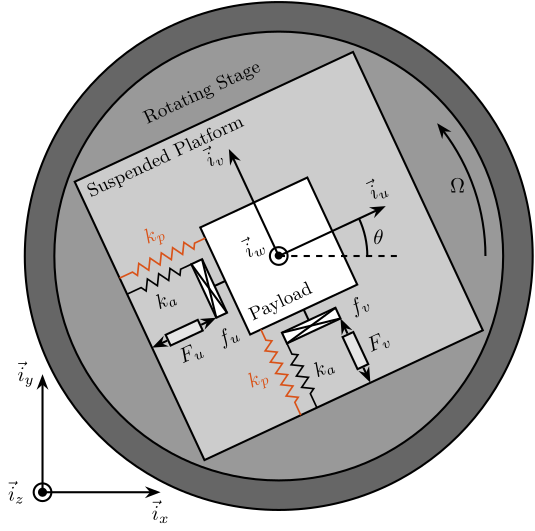

Studied system with additional springs in parallel with the actuators and force sensors (shown in red)

Equations

The forces measured by the two force sensors represented in Figure ref:fig:rotating_3dof_model_schematic_iff_parallel_springs are described by Eq. eqref:eq:measured_force_kp.

\begin{equation} \begin{bmatrix} f_{u} \\ f_{v} \end{bmatrix} = \begin{bmatrix} F_u \\ F_v \end{bmatrix} - (c s + k_a) \begin{bmatrix} d_u \\ d_v \end{bmatrix} \end{equation}

In order to keep the overall stiffness $k = k_a + k_p$ constant, thus not modifying the open-loop poles as $k_p$ is changed, a scalar parameter $\alpha$ ($0 \le \alpha < 1$) is defined to describe the fraction of the total stiffness in parallel with the actuator and force sensor as in Eq. eqref:eq:kp_alpha.

\begin{equation} k_p = \alpha k, \quad k_a = (1 - \alpha) k \end{equation}

After the equations of motion derived and transformed in the Laplace domain, the transfer function matrix $\mathbf{G}_k$ in Eq. eqref:eq:Gk_mimo_tf is computed. Its elements are shown in Eq. eqref:eq:Gk_diag and eqref:eq:Gk_off_diag.

\begin{equation} \begin{bmatrix} f_u \\ f_v \end{bmatrix} = \mathbf{G}_k \begin{bmatrix} F_u \\ F_v \end{bmatrix} \end{equation} \begin{subequations} \begin{align} \mathbf{G}_{k}(1,1) &= \mathbf{G}_{k}(2,2) = \frac{\big( \frac{s^2}{{\omega_0}^2} - \frac{\Omega^2}{{\omega_0}^2} + \alpha \big) \big( \frac{s^2}{{\omega_0}^2} + 2 \xi \frac{s}{\omega_0} + 1 - \frac{{\Omega}^2}{{\omega_0}^2} \big) + \big( 2 \frac{\Omega}{\omega_0} \frac{s}{\omega_0} \big)^2}{\big( \frac{s^2}{{\omega_0}^2} + 2 \xi \frac{s}{\omega_0} + 1 - \frac{{\Omega}^2}{{\omega_0}^2} \big)^2 + \big( 2 \frac{\Omega}{\omega_0} \frac{s}{\omega_0} \big)^2} \label{eq:Gk_diag} \\ \mathbf{G}_{k}(1,2) &= -\mathbf{G}_{k}(2,1) = \frac{- \left( 2 \xi \frac{s}{\omega_0} + 1 - \alpha \right) \left( 2 \frac{\Omega}{\omega_0} \frac{s}{\omega_0} \right)}{\left( \frac{s^2}{{\omega_0}^2} + 2 \xi \frac{s}{\omega_0} + 1 - \frac{{\Omega}^2}{{\omega_0}^2} \right)^2 + \left( 2 \frac{\Omega}{\omega_0} \frac{s}{\omega_0} \right)^2} \label{eq:Gk_off_diag} \end{align} \end{subequations}

Comparing $\mathbf{G}_k$ in Eq. eqref:eq:Gk with $\mathbf{G}_f$ in Eq. eqref:eq:Gf shows that while the poles of the system are kept the same, the zeros of the diagonal terms have changed. The two real zeros $z_r$ in Eq. eqref:eq:iff_zero_real that were inducing a non-minimum phase behavior are transformed into two complex conjugate zeros if the condition in Eq. eqref:eq:kp_cond_cc_zeros holds.

\begin{equation} \boxed{\alpha > \frac{\Omega^2}{{\omega_0}^2} \quad \Leftrightarrow \quad k_p > m \Omega^2} \end{equation}

Thus, if the added parallel stiffness $k_p$ is higher than the negative stiffness induced by centrifugal forces $m \Omega^2$, the dynamics from actuator to its collocated force sensor will show minimum phase behavior.

Effect of the parallel stiffness on the IFF plant

The IFF plant (transfer function from $[F_u, F_v]$ to $[f_u, f_v]$) is identified in three different cases:

• without parallel stiffness $k_p = 0$
• with a small parallel stiffness $k_p < m \Omega^2$
• with a large parallel stiffness $k_p > m \Omega^2$

Wz = 0.1; % The rotation speed [rad/s]

%% No parallel Stiffness
kp = 0; % Parallel Stiffness [N/m]
cp = 0.001*2*sqrt(kp*(mn+ms)); % Small parallel damping [N/(m/s)]
kn = 1 - kp; % Stiffness [N/m]
cn = 0.01*2*sqrt(kn*(mn+ms)); % Damping [N/(m/s)]

G_no_kp = linearize(mdl, io, 0);
G_no_kp.InputName = {'Fu', 'Fv', 'Fdx', 'Fdy'};
G_no_kp.OutputName = {'fu', 'fv', 'Du', 'Dv', 'Dx', 'Dy'};

%% Small parallel Stiffness
kp = 0.5*(mn+ms)*Wz^2; % Parallel Stiffness [N/m]
cp = 0.001*2*sqrt(kp*(mn+ms)); % Small parallel damping [N/(m/s)]
kn = 1 - kp; % Stiffness [N/m]
cn = 0.01*2*sqrt(kn*(mn+ms)); % Damping [N/(m/s)]

G_low_kp = linearize(mdl, io, 0);
G_low_kp.InputName = {'Fu', 'Fv', 'Fdx', 'Fdy'};
G_low_kp.OutputName = {'fu', 'fv', 'Du', 'Dv', 'Dx', 'Dy'};

%% Large parallel Stiffness
kp = 1.5*(mn+ms)*Wz^2; % Parallel Stiffness [N/m]
cp = 0.001*2*sqrt(kp*(mn+ms)); % Small parallel damping [N/(m/s)]
kn = 1 - kp; % Stiffness [N/m]
cn = 0.01*2*sqrt(kn*(mn+ms)); % Damping [N/(m/s)]

G_high_kp = linearize(mdl, io, 0);
G_high_kp.InputName = {'Fu', 'Fv', 'Fdx', 'Fdy'};
G_high_kp.OutputName = {'fu', 'fv', 'Du', 'Dv', 'Dx', 'Dy'};

The Bode plots of the obtained dynamics are shown in Figure ref:fig:rotating_iff_effect_kp. One can see that for $k_p > m \Omega^2$, the two real zeros with $k_p < m \Omega^2$ are transformed into two complex conjugate zeros and the systems shows alternating complex conjugate poles and zeros.

%% Effect of the parallel stiffness on the IFF plant
freqs = logspace(-2, 1, 1000);

figure;
tiledlayout(3, 1, 'TileSpacing', 'Compact', 'Padding', 'None');

% Magnitude
ax1 = nexttile([2, 1]);
hold on;
plot(freqs, abs(squeeze(freqresp(G_no_kp(  'fu', 'Fu'), freqs, 'rad/s'))), '-', ...
     'DisplayName', '$k_p = 0$')
plot(freqs, abs(squeeze(freqresp(G_low_kp( 'fu', 'Fu'), freqs, 'rad/s'))), '-', ...
     'DisplayName', '$k_p < m\Omega^2$')
plot(freqs, abs(squeeze(freqresp(G_high_kp('fu', 'Fu'), freqs, 'rad/s'))), '-', ...
     'DisplayName', '$k_p > m\Omega^2$')
hold off;
set(gca, 'XScale', 'log'); set(gca, 'YScale', 'log');
set(gca, 'XTickLabel',[]); ylabel('Magnitude [N/N]');
ylim([1e-5, 5e1]);
legend('location', 'southeast', 'FontSize', 8);

% Phase
ax2 = nexttile;
hold on;
plot(freqs, 180/pi*angle(squeeze(freqresp(G_no_kp(  'fu', 'Fu'), freqs, 'rad/s'))), '-')
plot(freqs, 180/pi*angle(squeeze(freqresp(G_low_kp( 'fu', 'Fu'), freqs, 'rad/s'))), '-')
plot(freqs, 180/pi*angle(squeeze(freqresp(G_high_kp('fu', 'Fu'), freqs, 'rad/s'))), '-')
set(gca, 'XScale', 'log'); set(gca, 'YScale', 'lin');
xlabel('Frequency [rad/s]'); ylabel('Phase [deg]');
yticks(-180:90:180);
ylim([-180 180]);
hold off;
xticks([1e-2,1e-1,1,1e1])
xticklabels({'$0.01 \omega_0$', '$0.1 \omega_0$', '$\omega_0$', '$10 \omega_0$'})

linkaxes([ax1,ax2],'x');
xlim([freqs(1), freqs(end)]);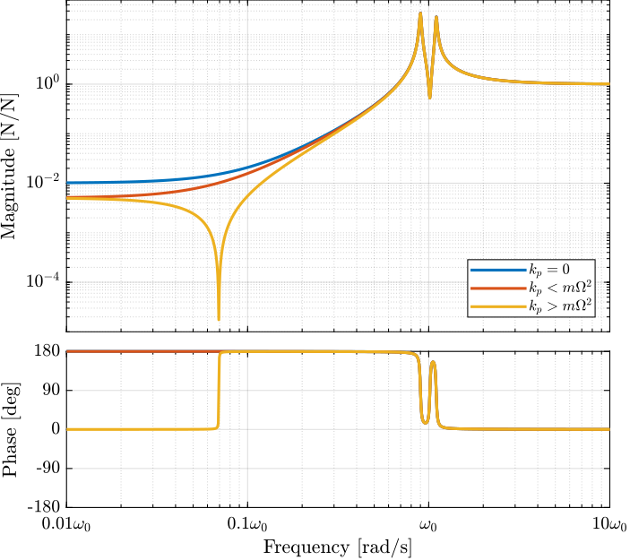

Effect of the parallel stiffness on the IFF plant: Bode plot of $G_{k}(1,1) = f_u/F_u$ without parallel spring, with parallel spring stiffness $k_p < m \Omega^2$ and $k_p > m \Omega^2$, $\Omega = 0.1 \omega_0$

Figure ref:fig:rotating_iff_kp_root_locus shows the Root Locus plots for $k_p = 0$, $k_p < m \Omega^2$ and $k_p > m \Omega^2$ when $K_F$ is a pure integrator as in Eq. eqref:eq:Kf_pure_int. It is shown that if the added stiffness is higher than the maximum negative stiffness, the poles of the closed-loop system are bounded on the (stable) left half-plane, and hence the unconditional stability of IFF is recovered.

%% Root Locus for IFF without parallel spring, with small parallel spring and with large parallel spring
gains = logspace(-2, 2, 200);

figure;
tiledlayout(1, 3, 'TileSpacing', 'Compact', 'Padding', 'None');

ax1 = nexttile([1,2]);
hold on;
plot(real(pole(G_no_kp({'fu','fv'},{'Fu','Fv'})*(1/s))),  imag(pole(G_no_kp({'fu','fv'},{'Fu','Fv'})*(1/s))), 'x', 'color', colors(1,:), ...
     'DisplayName', '$k_p = 0$','MarkerSize',8);
plot(real(tzero(G_no_kp({'fu','fv'},{'Fu','Fv'})*(1/s))),  imag(tzero(G_no_kp({'fu','fv'},{'Fu','Fv'})*(1/s))), 'o', 'color', colors(1,:), ...
     'HandleVisibility', 'off','MarkerSize',8);
for g = gains
    cl_poles = pole(feedback(G_no_kp({'fu','fv'},{'Fu','Fv'}), (g/s)*eye(2)));
    plot(real(cl_poles), imag(cl_poles), '.', 'color', colors(1,:), ...
         'HandleVisibility', 'off','MarkerSize',4);
end

plot(real(pole(G_low_kp({'fu','fv'},{'Fu','Fv'})*(1/s))),  imag(pole(G_low_kp({'fu','fv'},{'Fu','Fv'})*(1/s))), 'x', 'color', colors(2,:), ...
     'DisplayName', '$k_p < m\Omega^2$','MarkerSize',8);
plot(real(tzero(G_low_kp({'fu','fv'},{'Fu','Fv'})*(1/s))),  imag(tzero(G_low_kp({'fu','fv'},{'Fu','Fv'})*(1/s))), 'o', 'color', colors(2,:), ...
     'HandleVisibility', 'off','MarkerSize',8);
for g = gains
    cl_poles = pole(feedback(G_low_kp({'fu','fv'},{'Fu','Fv'}), (g/s)*eye(2)));
    plot(real(cl_poles), imag(cl_poles), '.', 'color', colors(2,:), ...
         'HandleVisibility', 'off','MarkerSize',4);
end

plot(real(pole(G_high_kp({'fu','fv'},{'Fu','Fv'})*(1/s))),  imag(pole(G_high_kp({'fu','fv'},{'Fu','Fv'})*(1/s))), 'x', 'color', colors(3,:), ...
     'DisplayName', '$k_p > m\Omega^2$','MarkerSize',8);
plot(real(tzero(G_high_kp({'fu','fv'},{'Fu','Fv'})*(1/s))),  imag(tzero(G_high_kp({'fu','fv'},{'Fu','Fv'})*(1/s))), 'o', 'color', colors(3,:), ...
     'HandleVisibility', 'off','MarkerSize',8);
for g = gains
    cl_poles = pole(feedback(G_high_kp({'fu','fv'},{'Fu','Fv'}), (g/s)*eye(2)));
    plot(real(cl_poles), imag(cl_poles), '.', 'color', colors(3,:), ...
         'HandleVisibility', 'off','MarkerSize',4);
end
hold off;
axis square;
xlim([-2.25, 0.25]); ylim([-1.25, 1.25]);
xticks([-2, -1, 0])
xticklabels({'$-2\omega_0$', '$-\omega_0$', '$0$'})
yticks([-1, 0, 1])
yticklabels({'$-\omega_0$', '$0$', '$\omega_0$'})

xlabel('Real Part'); ylabel('Imaginary Part');
leg = legend('location', 'northwest', 'FontSize', 8);
leg.ItemTokenSize(1) = 8;

ax2 = nexttile();
hold on;
plot(real(pole(G_no_kp( {'fu','fv'},{'Fu','Fv'})*(1/s))),  imag(pole(G_no_kp( {'fu','fv'},{'Fu','Fv'})*(1/s))), 'x', 'color', colors(1,:), 'MarkerSize',8);
plot(real(tzero(G_no_kp({'fu','fv'},{'Fu','Fv'})*(1/s))),  imag(tzero(G_no_kp({'fu','fv'},{'Fu','Fv'})*(1/s))), 'o', 'color', colors(1,:), 'MarkerSize',8);
for g = gains
    cl_poles = pole(feedback(G_no_kp({'fu','fv'},{'Fu','Fv'}), (g/s)*eye(2)));
    plot(real(cl_poles), imag(cl_poles), '.', 'color', colors(1,:), 'MarkerSize', 4);
end

plot(real(pole(G_low_kp( {'fu','fv'},{'Fu','Fv'})*(1/s))),  imag(pole(G_low_kp( {'fu','fv'},{'Fu','Fv'})*(1/s))), 'x', 'color', colors(2,:), 'MarkerSize',8);
plot(real(tzero(G_low_kp({'fu','fv'},{'Fu','Fv'})*(1/s))),  imag(tzero(G_low_kp({'fu','fv'},{'Fu','Fv'})*(1/s))), 'o', 'color', colors(2,:), 'MarkerSize',8);
for g = gains
    cl_poles = pole(feedback(G_low_kp({'fu','fv'},{'Fu','Fv'}), (g/s)*eye(2)));
    plot(real(cl_poles), imag(cl_poles), '.', 'color', colors(2,:), 'MarkerSize', 4);
end

plot(real(pole(G_high_kp( {'fu','fv'},{'Fu','Fv'})*(1/s))),  imag(pole(G_high_kp( {'fu','fv'},{'Fu','Fv'})*(1/s))), 'x', 'color', colors(3,:), 'MarkerSize',8);
plot(real(tzero(G_high_kp({'fu','fv'},{'Fu','Fv'})*(1/s))),  imag(tzero(G_high_kp({'fu','fv'},{'Fu','Fv'})*(1/s))), 'o', 'color', colors(3,:), 'MarkerSize',8);
for g = gains
    cl_poles = pole(feedback(G_high_kp({'fu','fv'},{'Fu','Fv'}), (g/s)*eye(2)));
    plot(real(cl_poles), imag(cl_poles), '.', 'color', colors(3,:), 'MarkerSize',4);
end
hold off;
axis equal;
xlim([-0.04, 0.04]); ylim([-0.08, 0.08]);
set(gca, 'XTickLabel',[]); set(gca, 'YTickLabel',[]);
xlabel('Real Part'); ylabel('Imaginary Part');
title('Zoom on controller pole')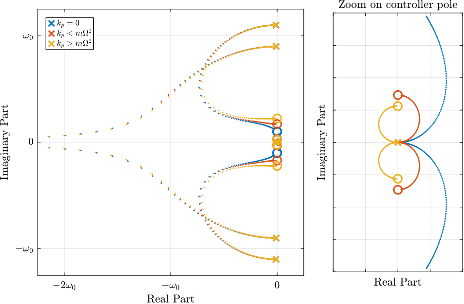

Root Locus for IFF without parallel spring, with small parallel spring and with large parallel spring

Effect of $k_p$ on the attainable damping

Even though the parallel stiffness $k_p$ has no impact on the open-loop poles (as the overall stiffness $k$ is kept constant), it has a large impact on the transmission zeros. Moreover, as the attainable damping is generally proportional to the distance between poles and zeros cite:preumont18_vibrat_contr_activ_struc_fourt_edition, the parallel stiffness $k_p$ is foreseen to have some impact on the attainable damping.

To study this effect, Root Locus plots for several parallel stiffnesses $k_p > m \Omega^2$ are shown in Figure ref:fig:rotating_iff_kp_root_locus_effect_kp. The frequencies of the transmission zeros of the system are increasing with an increase of the parallel stiffness $k_p$ (thus getting closer to the poles) and the associated attainable damping is reduced.

Therefore, even though the parallel stiffness $k_p$ should be larger than $m \Omega^2$ for stability reasons, it should not be taken too large as this would limit the attainable damping.

%% Tested parallel stiffnesses
kps = [2, 20, 40]*(mn + ms)*Wz^2;

%% Root Locus: Effect of the parallel stiffness on the attainable damping
figure;

gains = logspace(-2, 4, 500);

hold on;
for kp_i = 1:length(kps)
    kp = kps(kp_i); % Parallel Stiffness [N/m]
    cp = 0.001*2*sqrt(kp*(mn+ms)); % Small parallel damping [N/(m/s)]
    kn = 1 - kp; % Stiffness [N/m]
    cn = 0.01*2*sqrt(kn*(mn+ms)); % Damping [N/(m/s)]

    % Identify dynamics
    G = linearize(mdl, io, 0);
    G.InputName = {'Fu', 'Fv', 'Fdx', 'Fdy'};
    G.OutputName = {'fu', 'fv', 'Du', 'Dv', 'Dx', 'Dy'};

    plot(real(pole(G({'fu', 'fv'}, {'Fu', 'Fv'})*(1/s*eye(2)))),  imag(pole(G({'fu', 'fv'}, {'Fu', 'Fv'})*(1/s*eye(2)))), 'x', 'color', colors(kp_i,:), ...
         'DisplayName', sprintf('$k_p = %.1f m \\Omega^2$', kp/((mn+ms)*Wz^2)),'MarkerSize',8);
    plot(real(tzero(G({'fu', 'fv'}, {'Fu', 'Fv'})*(1/s*eye(2)))),  imag(tzero(G({'fu', 'fv'}, {'Fu', 'Fv'})*(1/s*eye(2)))), 'o', 'color', colors(kp_i,:), ...
         'HandleVisibility', 'off','MarkerSize',8);
    for g = gains
        cl_poles = pole(feedback(G({'fu', 'fv'}, {'Fu', 'Fv'}), (g/s)*eye(2)));
        plot(real(cl_poles), imag(cl_poles), '.', 'color', colors(kp_i,:),'MarkerSize',4, ...
             'HandleVisibility', 'off');
    end
end
hold off;
axis square;
% xlim([-1.15, 0.05]); ylim([0, 1.2]);
xlim([-2.25, 0.25]); ylim([-1.25, 1.25]);
xticks([-2, -1, 0])
xticklabels({'$-2\omega_0$', '$-\omega_0$', '$0$'})
yticks([-1, 0, 1])
yticklabels({'$-\omega_0$', '$0$', '$\omega_0$'})

xlabel('Real Part'); ylabel('Imaginary Part');
leg = legend('location', 'northwest', 'FontSize', 8);
leg.ItemTokenSize(1) = 12;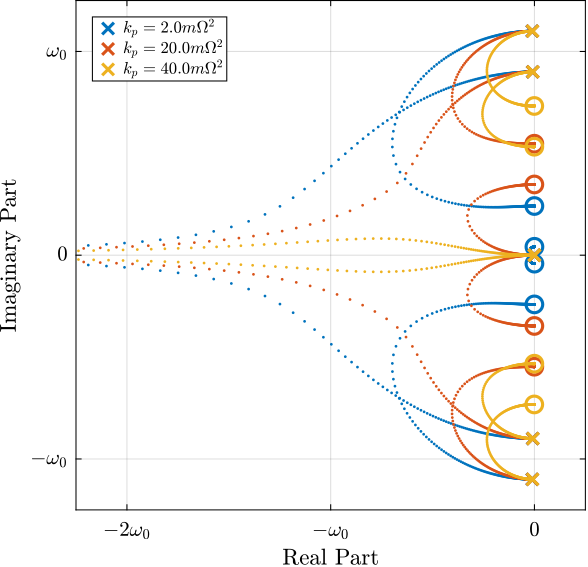

Root Locus: Effect of the parallel stiffness on the attainable damping, $\Omega = 0.1 \omega_0$

This is confirmed by the Figure ref:fig:rotating_iff_kp_optimal_gain where the attainable closed-loop damping ratio $\xi_{\text{cl}}$ and the associated optimal control gain $g_\text{opt}$ are computed as a function of the parallel stiffness.

%% Computes the optimal parameters and attainable simultaneous damping
alphas = logspace(-2, 0, 100);
alphas(end) = []; % Remove last point

opt_xi = zeros(1, length(alphas)); % Optimal simultaneous damping
opt_gain = zeros(1, length(alphas)); % Corresponding optimal gain

Kiff = 1/s*eye(2);

for alpha_i = 1:length(alphas)
    kp = alphas(alpha_i);
    cp = 0.001*2*sqrt(kp*(mn+ms)); % Small parallel damping [N/(m/s)]
    kn = 1 - kp; % Stiffness [N/m]
    cn = 0.01*2*sqrt(kn*(mn+ms)); % Damping [N/(m/s)]

    % Identify dynamics
    G = linearize(mdl, io, 0);
    G.InputName = {'Fu', 'Fv', 'Fdx', 'Fdy'};
    G.OutputName = {'fu', 'fv', 'Du', 'Dv', 'Dx', 'Dy'};

    fun = @(g)computeSimultaneousDamping(g, G({'fu', 'fv'}, {'Fu', 'Fv'}), Kiff);

    [g_opt, xi_opt] = fminsearch(fun, 2);
    opt_xi(alpha_i) = 1/xi_opt;
    opt_gain(alpha_i) = g_opt;
end

%% Attainable damping as a function of the stiffness ratio
figure;
yyaxis left
plot(alphas, opt_xi, '-', 'DisplayName', '$\xi_{cl}$');
set(gca, 'YScale', 'lin');
ylim([0,1]);
ylabel('Damping Ratio $\xi$');

yyaxis right
hold on;
plot(alphas, opt_gain, '-', 'DisplayName', '$g_{opt}$');
set(gca, 'YScale', 'lin');
ylim([0,2.5]);
ylabel('Controller gain $g$');

set(gca, 'XScale', 'log');
legend('location', 'northeast', 'FontSize', 8);

xlabel('$k_p$');
xlim([0.01, 1]);
xticks([0.01, 0.1, 1])
xticklabels({'$m\Omega^2$', '$10m\Omega^2$', '$100m\Omega^2$'})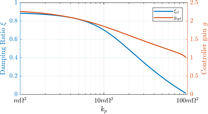

Attainable damping ratio $\xi_\text{cl}$ as a function of the parallel stiffness $k_p$. Corresponding control gain $g_\text{opt}$ is also shown. Values for $k_p < m\Omega^2$ are not shown as the system is unstable.

Damped plant

Let's choose a parallel stiffness equal to $k_p = 2 m \Omega^2$ and compute the damped plant. The damped and undamped transfer functions from $F_u$ to $d_u$ are compared in Figure ref:fig:rotating_iff_kp_damped_plant.

Even though the two resonances are well damped, the IFF changes the low frequency behavior of the plant which is usually not wanted. This is due to the fact that "pure" integrators are used, and that the low frequency loop gains becomes large below some frequency.

%% Identify dynamics with parallel stiffness = 2mW^2
Wz = 0.1; % [rad/s]
kp = 2*(mn + ms)*Wz^2; % Parallel Stiffness [N/m]
cp = 0.001*2*sqrt(kp*(mn+ms)); % Small parallel damping [N/(m/s)]
kn = 1 - kp; % Stiffness [N/m]
cn = 0.01*2*sqrt(kn*(mn+ms)); % Damping [N/(m/s)]

% Identify dynamics
G = linearize(mdl, io, 0);
G.InputName = {'Fu', 'Fv', 'Fdx', 'Fdy'};
G.OutputName = {'fu', 'fv', 'Du', 'Dv', 'Dx', 'Dy'};

%% IFF controller with pure integrator
Kiff_kp = (2.2/s)*eye(2);
Kiff_kp.InputName = {'fu', 'fv'};
Kiff_kp.OutputName = {'Fu', 'Fv'};

%% Compute the damped plant
G_cl_iff_kp = feedback(G, Kiff_kp, 'name');

%% Damped plant with IFF - Transfer function from $F_u$ to $d_u$
freqs = logspace(-3, 1, 1000);

figure;
tiledlayout(3, 1, 'TileSpacing', 'Compact', 'Padding', 'None');

% Magnitude
ax1 = nexttile([2, 1]);
hold on;
plot(freqs, abs(squeeze(freqresp(G('Du', 'Fu'), freqs, 'rad/s'))), '-', 'color', zeros(1,3), ...
    'DisplayName', '$d_u/F_u$ - OL')
plot(freqs, abs(squeeze(freqresp(G_cl_iff_kp('Du', 'Fu'), freqs, 'rad/s'))), '-', 'color', colors(1,:), ...
    'DisplayName', '$d_u/F_u$ - IFF + $k_p$')
plot(freqs, abs(squeeze(freqresp(G('Dv', 'Fu'), freqs, 'rad/s'))), '-', 'color', [zeros(1,3), 0.5], ...
    'DisplayName', '$d_v/F_u$ - OL')
plot(freqs, abs(squeeze(freqresp(G_cl_iff_kp('Dv', 'Fu'), freqs, 'rad/s'))), '-', 'color', [colors(1,:), 0.5], ...
    'DisplayName', '$d_v/F_u$ - IFF + $k_p$')
hold off;
set(gca, 'XScale', 'log'); set(gca, 'YScale', 'log');
set(gca, 'XTickLabel',[]); ylabel('Magnitude [m/N]');
ldg = legend('location', 'southwest', 'FontSize', 8, 'NumColumns', 2);
ldg.ItemTokenSize(1) = 20;
ylim([1e-6, 1e2]);

ax2 = nexttile;
hold on;
plot(freqs, 180/pi*angle(squeeze(freqresp(G('Du', 'Fu'), freqs, 'rad/s'))), '-', 'color', zeros(1,3))
plot(freqs, 180/pi*angle(squeeze(freqresp(G_cl_iff_kp('Du', 'Fu'), freqs, 'rad/s'))), '-', 'color', colors(1,:))
hold off;
set(gca, 'XScale', 'log'); set(gca, 'YScale', 'lin');
xlabel('Frequency [rad/s]'); ylabel('Phase [deg]');
yticks(-180:90:180);
ylim([-180 180]);
xticks([1e-3,1e-2,1e-1,1,1e1])
xticklabels({'$0.001 \omega_0$', '$0.01 \omega_0$', '$0.1 \omega_0$', '$\omega_0$', '$10 \omega_0$'})

linkaxes([ax1,ax2],'x');
xlim([freqs(1), freqs(end)]);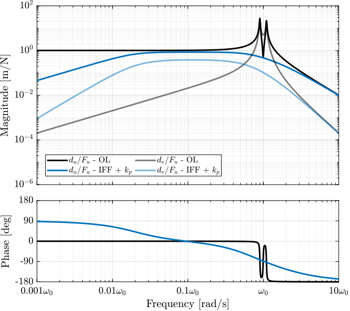

Damped plant with IFF - Transfer function from $F_u$ to $d_u$

In order to lower the low frequency gain, an high pass filter is added to the IFF controller (which is equivalent as shifting the controller pole to the left in the complex plane):

\begin{equation} K_{\text{IFF}}(s) = g\frac{1}{\omega_i + s} \begin{bmatrix} 1 & 0 \\ 0 & 1 \end{bmatrix} \end{equation}

Let's see how the high pass filter impacts the attainable damping. The controller gain $g$ is kept constant while $\omega_i$ is changed, and the minimum damping ratio of the damped plant is computed. The obtained damping ratio as a function of $\omega_i/\omega_0$ (where $\omega_0$ is the resonance of the system without rotation) is shown in Figure ref:fig:rotating_iff_kp_added_hpf_effect_damping.

w0 = sqrt((kn+kp)/(mn+ms)); % Resonance frequency [rad/s]
wis = w0*logspace(-2, 0, 100); % LPF cut-off [rad/s]

%% Computes the obtained damping as a function of the HPF cut-off frequency
opt_xi = zeros(1, length(wis)); % Optimal simultaneous damping

for wi_i = 1:length(wis)
    Kiff_kp_hpf = (2.2/(s + wis(wi_i)))*eye(2);
    Kiff_kp_hpf.InputName = {'fu', 'fv'};
    Kiff_kp_hpf.OutputName = {'Fu', 'Fv'};

    [~, xi] = damp(feedback(G, Kiff_kp_hpf, 'name'));
    opt_xi(wi_i) = min(xi);
end

%% Effect of the high pass filter cut-off frequency on the obtained damping
figure;
plot(wis, opt_xi, '-');
set(gca, 'XScale', 'log');
set(gca, 'YScale', 'lin');
ylim([0,1]);
ylabel('Damping Ratio $\xi$');
xlabel('$\omega_i/\omega_0$');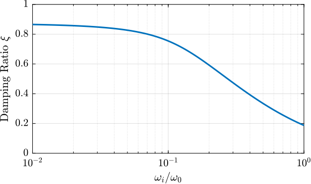

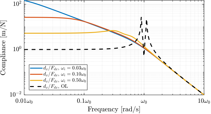
Effect of the high pass filter cut-off frequency on the obtained damping

Let's choose $\omega_i = 0.1 \cdot \omega_0$ and compute the damped plant again. The Bode plots of the undamped, damped with "pure" IFF, and with added high pass filters are shown in Figure ref:fig:rotating_iff_kp_added_hpf_damped_plant. The added high pass filter gives almost the same damping properties while giving acceptable low frequency behavior.

%% Compute the damped plant with added High Pass Filter
Kiff_kp_hpf = (2.2/(s + 0.1*w0))*eye(2);
Kiff_kp_hpf.InputName = {'fu', 'fv'};
Kiff_kp_hpf.OutputName = {'Fu', 'Fv'};

G_cl_iff_hpf_kp = feedback(G, Kiff_kp_hpf, 'name');

%% Bode plot of the direct and coupling terms for several rotating velocities
freqs = logspace(-3, 1, 1000);

figure;
tiledlayout(3, 1, 'TileSpacing', 'Compact', 'Padding', 'None');

% Magnitude
ax1 = nexttile([2, 1]);
hold on;
plot(freqs, abs(squeeze(freqresp(G(              'Du', 'Fu'), freqs, 'rad/s'))), '-', 'color', zeros( 1,3), ...
    'DisplayName', '$d_u/F_u$ - OL')
plot(freqs, abs(squeeze(freqresp(G_cl_iff_kp(    'Du', 'Fu'), freqs, 'rad/s'))), '-', 'color', colors(1,:), ...
    'DisplayName', '$d_u/F_u$ - IFF + $k_p$')
plot(freqs, abs(squeeze(freqresp(G_cl_iff_hpf_kp('Du', 'Fu'), freqs, 'rad/s'))), '-', 'color', colors(2,:), ...
    'DisplayName', '$d_u/F_u$ - IFF + $k_p$ + HPF')
plot(freqs, abs(squeeze(freqresp(G(              'Dv', 'Fu'), freqs, 'rad/s'))), '-', 'color', [zeros( 1,3), 0.5], ...
    'DisplayName', '$d_v/F_u$ - OL')
plot(freqs, abs(squeeze(freqresp(G_cl_iff_kp(    'Dv', 'Fu'), freqs, 'rad/s'))), '-', 'color', [colors(1,:), 0.5], ...
    'DisplayName', '$d_v/F_u$ - IFF + $k_p$')
plot(freqs, abs(squeeze(freqresp(G_cl_iff_hpf_kp('Dv', 'Fu'), freqs, 'rad/s'))), '-', 'color', [colors(2,:), 0.5], ...
    'DisplayName', '$d_v/F_u$ - IFF + $k_p$ + HPF')
hold off;
set(gca, 'XScale', 'log'); set(gca, 'YScale', 'log');
set(gca, 'XTickLabel',[]); ylabel('Magnitude [m/N]');
ldg = legend('location', 'southwest', 'FontSize', 8, 'NumColumns', 2);
ldg.ItemTokenSize(1) = 20;

ax2 = nexttile;
hold on;
plot(freqs, 180/pi*angle(squeeze(freqresp(G(              'Du', 'Fu'), freqs, 'rad/s'))), '-', 'color', zeros( 1,3))
plot(freqs, 180/pi*angle(squeeze(freqresp(G_cl_iff_kp(    'Du', 'Fu'), freqs, 'rad/s'))), '-', 'color', colors(1,:))
plot(freqs, 180/pi*angle(squeeze(freqresp(G_cl_iff_hpf_kp('Du', 'Fu'), freqs, 'rad/s'))), '-', 'color', colors(2,:))
hold off;
set(gca, 'XScale', 'log'); set(gca, 'YScale', 'lin');
xlabel('Frequency [rad/s]'); ylabel('Phase [deg]');
yticks(-180:90:180);
ylim([-180 180]);
xticks([1e-3,1e-2,1e-1,1,1e1])
xticklabels({'$0.001 \omega_0$', '$0.01 \omega_0$', '$0.1 \omega_0$', '$\omega_0$', '$10 \omega_0$'})

linkaxes([ax1,ax2],'x');
xlim([freqs(1), freqs(end)]);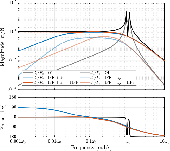

Damped plant with IFF - Transfer function from $F_u$ to $d_u$

Relative Damping Control

<<sec:rotating_relative_damp_control>>

Introduction   ignore

In order to apply a "relative damping control strategy", relative motion sensors are added in parallel with the actuators as shown in Figure ref:fig:rotating_3dof_model_schematic_rdc.

Two controllers $K_d$ are used to fed back the relative motion to the actuator. $K_d$ is a derivator:

\begin{equation} K_d(s) = s \end{equation}

To be implemented in practice, it is usually replaced by a an high pass filter:

\begin{equation} K_d(s) = \frac{s}{s + \omega_d} \end{equation}

\begin{tikzpicture}
  % Angle
  \def\thetau{25}

  % Rotational Stage
  \draw[fill=black!60!white] (0, 0) circle (4.3);
  \draw[fill=black!40!white] (0, 0) circle (3.8);

  % Label
  \node[anchor=north west, rotate=\thetau] at (-2.5, 2.5) {\small Rotating Stage};

  % Rotating Scope
  \begin{scope}[rotate=\thetau]
    % Rotating Frame
    \draw[fill=black!20!white] (-2.6, -2.6) rectangle (2.6, 2.6);
    % Label
    \node[anchor=north west, rotate=\thetau] at (-2.6, 2.6) {\small Suspended Platform};

    % Mass
    \draw[fill=white] (-1, -1) rectangle (1, 1);
    % Label
    \node[anchor=south west, rotate=\thetau] at (-1, -1) {\small Payload};

    % Attached Points
    \node[] at (-1, 0){$\bullet$};
    \draw[] (-1, 0) -- ++(-0.2, 0) coordinate(cu);
    \draw[] ($(cu) + (0, -0.8)$) coordinate(actu) -- ($(cu) + (0, 0.8)$) coordinate(ku);
    \node[] at (0, -1){$\bullet$};
    \draw[] (0, -1) -- ++(0, -0.2) coordinate(cv);
    \draw[] ($(cv) + (-0.8, 0)$)coordinate(kv) -- ($(cv) + (0.8, 0)$) coordinate(actv);

    % Spring and Actuator for U
    \draw[actuator={0.6}{0.2}{black}] (cu) -- coordinate[midway, below=0.1](actumid) node[above=0.1, rotate=\thetau]{$F_u$} (cu-|-2.6,0);
    \draw[spring=0.2] (ku) -- node[above=0.1, rotate=\thetau]{$k$} (ku-|-2.6,0);
    \draw[<->, dashed, draw=coloryellow] (actu) node[below=0.1, rotate=\thetau, color=coloryellow](du){$d_u$} -- (actu-|-2.6,0);

    \node[color=coloryellow, block={0.6cm}{0.6cm}, fill=coloryellow!10!white, rotate=\thetau] (Ku) at ($(actumid) + (0, -1.4)$) {$K_{d}$};
    \draw[->, draw=coloryellow] (du.south) -- ++(0, -0.8) -| (Ku.south);
    \draw[->, draw=coloryellow] (Ku.north) -- (actumid);

    \draw[actuator={0.6}{0.2}{black}] (cv) -- coordinate[midway, right=0.1](actvmid) node[left, rotate=\thetau]{$F_v$} (cv|-0,-2.6);
    \draw[spring=0.2] (kv) -- node[left, rotate=\thetau]{$k$} (kv|-0,-2.6);
    \draw[<->, dashed, draw=coloryellow] (actv)node[right=0.1, rotate=\thetau, color=coloryellow](dv){$d_v$} -- (actv|-0,-2.6);

    \node[color=coloryellow, block={0.6cm}{0.6cm}, fill=coloryellow!10!white, rotate=\thetau] (Kv) at ($(actvmid) + (1.4, 0)$) {$K_{d}$};
    \draw[->, draw=coloryellow] (dv.east) -- ++(0.8, 0) |- (Kv.east);
    \draw[->, draw=coloryellow] (Kv.west) -- (actvmid);
  \end{scope}

  % Inertial Frame
  \draw[->] (-4, -4) -- ++(2, 0) node[below]{$\vec{i}_x$};
  \draw[->] (-4, -4) -- ++(0, 2) node[left]{$\vec{i}_y$};
  \draw[fill, color=black] (-4, -4) circle (0.06);
  \node[draw, circle, inner sep=0pt, minimum size=0.3cm, label=left:$\vec{i}_z$] at (-4, -4){};

  \draw[->] (0, 0) node[above left, rotate=\thetau]{$\vec{i}_w$} -- ++(\thetau:2) node[above, rotate=\thetau]{$\vec{i}_u$};
  \draw[->] (0, 0) -- ++(\thetau+90:2) node[left, rotate=\thetau]{$\vec{i}_v$};
  \draw[fill, color=black] (0,0) circle (0.06);
  \node[draw, circle, inner sep=0pt, minimum size=0.3cm] at (0, 0){};
  \draw[dashed] (0, 0) -- ++(2, 0);
  \draw[] (1.5, 0) arc (0:\thetau:1.5) node[midway, right]{$\theta$};

  \draw[->] (3.5, 0) arc (0:40:3.5) node[midway, left]{$\Omega$};
\end{tikzpicture}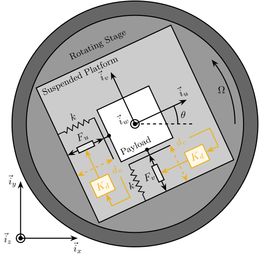

System with relative motion sensor and decentralized "relative damping control" applied.

Equations of motion

Let's note $\bm{G}_d$ the transfer function between actuator forces and measured relative motion in parallel with the actuators:

\begin{equation} \begin{bmatrix} d_u \\ d_v \end{bmatrix} = \mathbf{G}_d \begin{bmatrix} F_u \\ F_v \end{bmatrix} \end{equation}

With:

\begin{subequations} \begin{align} \mathbf{G}_{d}(1,1) &= \mathbf{G}_{d}(2,2) = \frac{\frac{1}{k} \left( \frac{s^2}{{\omega_0}^2} + 2 \xi \frac{s}{\omega_0} + 1 - \frac{{\Omega}^2}{{\omega_0}^2} \right)}{\left( \frac{s^2}{{\omega_0}^2} + 2 \xi \frac{s}{\omega_0} + 1 - \frac{{\Omega}^2}{{\omega_0}^2} \right)^2 + \left( 2 \frac{\Omega}{\omega_0} \frac{s}{\omega_0} \right)^2} \\ \mathbf{G}_{d}(1,2) &= -\mathbf{G}_{d}(2,1) = \frac{\frac{1}{k} \left( 2 \frac{\Omega}{\omega_0} \frac{s}{\omega_0} \right)}{\left( \frac{s^2}{{\omega_0}^2} + 2 \xi \frac{s}{\omega_0} + 1 - \frac{{\Omega}^2}{{\omega_0}^2} \right)^2 + \left( 2 \frac{\Omega}{\omega_0} \frac{s}{\omega_0} \right)^2} \end{align} \end{subequations}

Neglecting the damping for simplicity ($\xi \ll 1$), the direct terms have two complex conjugate zeros:

\begin{equation} z = \pm j \sqrt{\omega_0^2 - \omega^2} \end{equation}

Which are between the two pairs of complex conjugate poles at:

\begin{align} p_1 &= \pm j (\omega_0 - \omega) \\ p_2 &= \pm j (\omega_0 + \omega) \end{align}

Therefore, for $\Omega < \sqrt{k/m}$ (i.e. stable system), the transfer functions for Relative Damping Control have alternating complex conjugate poles and zeros.

Decentralized Relative Damping Control

The transfer functions from $[F_u,\ F_v]$ to $[d_u,\ d_v]$ is identified and shown in Figure ref:fig:rotating_rdc_plant_effect_rot for several rotating velocities.

%% Bode plot of the direct and coupling term for the "relative damping control" plant - Effect of rotation
figure;
freqs = logspace(-2, 1, 1000);

figure;
tiledlayout(3, 2, 'TileSpacing', 'Compact', 'Padding', 'None');

% Magnitude
ax1 = nexttile([2, 1]);
hold on;
for i = 1:length(Wzs)
    plot(freqs, abs(squeeze(freqresp(Gs{i}('du', 'Fu'), freqs, 'rad/s'))), '-', 'color', colors(i,:))
end
hold off;
set(gca, 'XScale', 'log'); set(gca, 'YScale', 'log');
set(gca, 'XTickLabel',[]); ylabel('Magnitude [N/N]');
title('Direct terms: $d_u/F_u$, $d_v/F_v$');
ylim([1e-3, 1e2]);

ax2 = nexttile([2, 1]);
hold on;
for i = 1:length(Wzs)
    plot(freqs, abs(squeeze(freqresp(Gs{i}('dv', 'Fu'), freqs, 'rad/s'))), '-', 'color', colors(i,:), ...
         'DisplayName', sprintf('$\\Omega = %.1f \\omega_0$', Wzs(i)))
end
hold off;
set(gca, 'XScale', 'log'); set(gca, 'YScale', 'log');
set(gca, 'XTickLabel',[]); set(gca, 'YTickLabel',[]);
title('Coupling Terms: $d_u/F_v$, $d_v/F_u$');
ldg = legend('location', 'northwest', 'FontSize', 8, 'NumColumns', 1);
ldg.ItemTokenSize = [10, 1];
ylim([1e-3, 1e2]);

ax3 = nexttile;
hold on;
for i = 1:length(Wzs)
    plot(freqs, 180/pi*angle(squeeze(freqresp(Gs{i}('du', 'Fu'), freqs, 'rad/s'))), '-', 'color', colors(i,:))
end
hold off;
set(gca, 'XScale', 'log'); set(gca, 'YScale', 'lin');
xlabel('Frequency [rad/s]'); ylabel('Phase [deg]');
yticks(-180:90:180);
ylim([-180 180]);
xticks([1e-2,1e-1,1,1e1])
xticklabels({'$0.01 \omega_0$', '$0.1 \omega_0$', '$\omega_0$', '$10 \omega_0$'})

ax4 = nexttile;
hold on;
for i = 1:length(Wzs)
    plot(freqs, 180/pi*angle(squeeze(freqresp(Gs{i}('dv', 'Fu'), freqs, 'rad/s'))), '-', 'color', colors(i,:));
end
hold off;
set(gca, 'XScale', 'log'); set(gca, 'YScale', 'lin');
xlabel('Frequency [rad/s]'); set(gca, 'YTickLabel',[]);
yticks(-180:90:180);
ylim([-180 180]);
xticks([1e-2,1e-1,1,1e1])
xticklabels({'$0.01 \omega_0$', '$0.1 \omega_0$', '$\omega_0$', '$10 \omega_0$'})

linkaxes([ax1,ax2,ax3,ax4],'x');
xlim([freqs(1), freqs(end)]);

linkaxes([ax1,ax2],'y');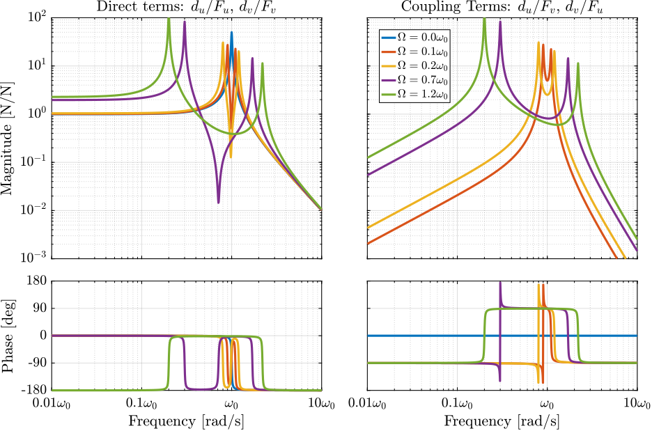

Bode plot of the direct and coupling term for the "relative damping control" plant - Effect of rotation

In order to see if large damping can be added with Relative Damping Control, the root locus is computed (Figure ref:fig:rotating_rdc_root_locus). The closed-loop system is unconditionally stable and the poles can be damped as much as wanted.

%% Root Locus for Relative Damping Control
figure;

Krdc = s*eye(2); % Relative damping controller

gains = logspace(-2, 2, 300); % Tested gains
Wz_i = [1,3,4];

hold on;
for i = 1:length(Wz_i)
    plot(real(pole(Gs{Wz_i(i)}({'du', 'dv'}, {'Fu', 'Fv'})*Krdc)),  imag(pole(Gs{Wz_i(i)}({'du', 'dv'}, {'Fu', 'Fv'})*Krdc)), 'x', 'color', colors(i,:), ...
         'DisplayName', sprintf('$\\Omega = %.1f \\omega_0 $', Wzs(Wz_i(i))),'MarkerSize',8);
    plot(real(tzero(Gs{Wz_i(i)}({'du', 'dv'}, {'Fu', 'Fv'})*Krdc)),  imag(tzero(Gs{Wz_i(i)}({'du', 'dv'}, {'Fu', 'Fv'})*Krdc)), 'o', 'color', colors(i,:), ...
         'HandleVisibility', 'off','MarkerSize',8);
    for g = gains
        cl_poles = pole(feedback(Gs{Wz_i(i)}({'du', 'dv'}, {'Fu', 'Fv'}), g*Krdc, -1));
        plot(real(cl_poles), imag(cl_poles), '.', 'color', colors(i,:), ...
             'HandleVisibility', 'off','MarkerSize',4);
    end
end
hold off;
axis square;
xlim([-1.8, 0.2]); ylim([0, 2]);
xticks([-1, 0])
xticklabels({'-$\omega_0$', '$0$'})
yticks([0, 1, 2])
yticklabels({'$0$', '$\omega_0$', '$2 \omega_0$'})

xlabel('Real Part'); ylabel('Imaginary Part');
leg = legend('location', 'northwest', 'FontSize', 8);
leg.ItemTokenSize(1) = 8;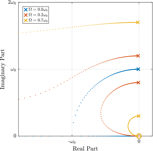

Root Locus for Relative Damping Control

Damped Plant

Let's select a reasonable "Relative Damping Control" gain, and compute the closed-loop damped system. The open-loop and damped plants are compared in Figure ref:fig:rotating_rdc_damped_plant.

The rotating aspect does not add any complexity for the use of Relative Damping Control. It does not increase the low frequency coupling as compared to Integral Force Feedback.

i = 2;

%% Relative Damping Controller
Krdc = 2*s*eye(2);
Krdc.InputName = {'Du', 'Dv'};
Krdc.OutputName = {'Fu', 'Fv'};

%% Compute the damped plant
G_cl_rdc = feedback(Gs{i}, Krdc, 'name');

%% Damped plant using Relative Damping Control
figure;
freqs = logspace(-3, 2, 1000);

figure;
tiledlayout(3, 1, 'TileSpacing', 'Compact', 'Padding', 'None');

% Magnitude
ax1 = nexttile([2, 1]);
hold on;
plot(freqs, abs(squeeze(freqresp(Gs{i}(   'Du', 'Fu'), freqs, 'rad/s'))), '-', 'color', zeros(1,3), ...
    'DisplayName', 'OL - $G_d(1,1)$')
plot(freqs, abs(squeeze(freqresp(G_cl_rdc('Du', 'Fu'), freqs, 'rad/s'))), '-', 'color', colors(1,:), ...
    'DisplayName', 'RDC - $G_d(1,1)$')
plot(freqs, abs(squeeze(freqresp(Gs{i}(   'Dv', 'Fu'), freqs, 'rad/s'))), '-', 'color', [zeros(1,3), 0.5], ...
    'DisplayName', 'OL - $G_d(2,1)$')
plot(freqs, abs(squeeze(freqresp(G_cl_rdc('Dv', 'Fu'), freqs, 'rad/s'))), '-', 'color', [colors(1,:), 0.5], ...
    'DisplayName', 'RDC - $G_d(2,1)$')
hold off;
set(gca, 'XScale', 'log'); set(gca, 'YScale', 'log');
set(gca, 'XTickLabel',[]); ylabel('Magnitude [m/N]');
ldg = legend('location', 'southwest', 'FontSize', 8, 'NumColumns', 2);
ldg.ItemTokenSize(1) = 20;
ylim([1e-6, 1e2]);

ax2 = nexttile;
hold on;
plot(freqs, 180/pi*angle(squeeze(freqresp(Gs{i}('Du', 'Fu'), freqs, 'rad/s'))), '-', 'color', zeros(1,3))
plot(freqs, 180/pi*angle(squeeze(freqresp(G_cl_rdc('Du', 'Fu'), freqs, 'rad/s'))), '-', 'color', colors(1,:))
hold off;
set(gca, 'XScale', 'log'); set(gca, 'YScale', 'lin');
xlabel('Frequency [rad/s]'); ylabel('Phase [deg]');
yticks(-180:90:180);
ylim([-180 180]);

linkaxes([ax1,ax2],'x');
xlim([freqs(1), freqs(end)]);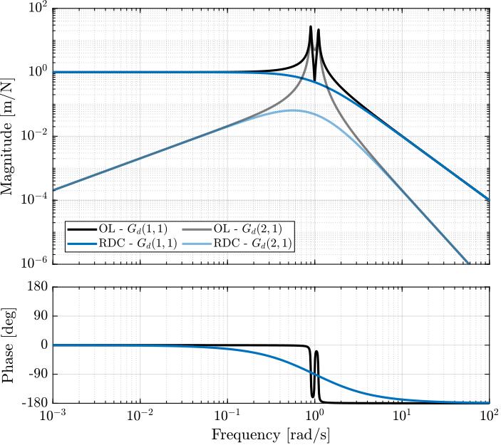

Damped plant using Relative Damping Control

Comparison of Active Damping Techniques

<<sec:rotating_comp_act_damp>>

Introduction   ignore

These two proposed IFF modifications as well as relative damping control are now compared in terms of added damping and closed-loop behavior.

For the following comparisons, the cut-off frequency for the added HPF is set to $\omega_i = 0.1 \omega_0$ and the stiffness of the parallel springs is set to $k_p = 5 m \Omega^2$ (corresponding to $\alpha = 0.05$). These values are chosen based on previous discussion about optimal parameters.

Root Locus

Figure ref:fig:rotating_comp_techniques_root_locus shows the Root Locus plots for the two proposed IFF modifications as well as for relative damping control. While the two pairs of complex conjugate open-loop poles are identical for both IFF modifications, the transmission zeros are not. This means that the closed-loop behavior of both systems will differ when large control gains are used.

One can observe that the closed loop poles corresponding to the system with added springs (in red) are bounded to the left half plane implying unconditional stability. This is not the case for the system where the controller is augmented with an HPF (in blue).

It is interesting to note that the maximum added damping is very similar for both techniques.

Comparison of active damping techniques for rotating platform - Root Locus

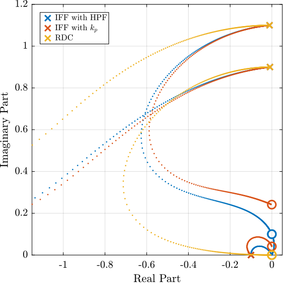
Obtained Damped Plant

The actively damped plants are computed for the three techniques and compared in Figure ref:fig:rotating_comp_techniques_dampled_plants.

It is shown that while the diagonal (direct) terms of the damped plants are similar for the three active damping techniques, of off-diagonal (coupling) terms are not. Integral Force Feedback strategy is adding some coupling at low frequency which may negatively impact the positioning performances.

%% Compute Damped plants
G_cl_iff    = feedback(G,    Kiff,    'name');
G_cl_iff_kp = feedback(G_kp, Kiff_kp, 'name');
G_cl_rdc    = feedback(G,    Krdc,    'name');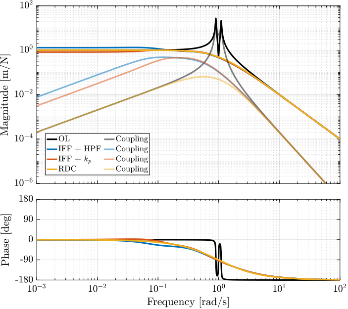

Comparison of the damped plants obtained with the three active damping techniques

Transmissibility And Compliance

The proposed active damping techniques are now compared in terms of closed-loop transmissibility and compliance.

The transmissibility is here defined as the transfer function from a displacement of the rotating stage along $\vec{i}_x$ to the displacement of the payload along the same direction. It is used to characterize how much vibration is transmitted through the suspended platform to the payload.

The compliance describes the displacement response of the payload to external forces applied to it. This is a useful metric when disturbances are directly applied to the payload. It is here defined as the transfer function from external forces applied on the payload along $\vec{i}_x$ to the displacement of the payload along the same direction.

Very similar results are obtained for the two proposed IFF modifications in terms of transmissibility and compliance (Figure ref:fig:rotating_comp_techniques_transmissibility_compliance).

Using IFF degrades the compliance at low frequency while using relative damping control degrades the transmissibility at high frequency. This is very well known characteristics of these common active damping techniques that holds when applied to rotating platforms.

Comparison of the obtained transmissibilty and compliance for the three tested active damping techniques

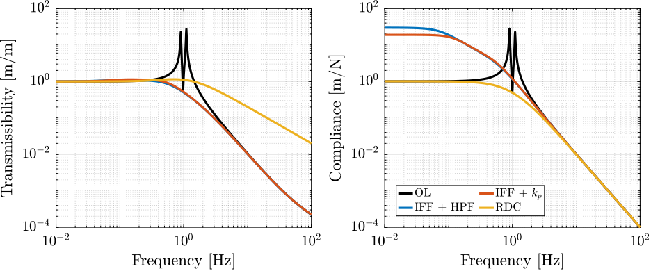
Rotating Nano-Hexapod

<<sec:rotating_nano_hexapod>>

Introduction   ignore

The current analysis is now applied on a model representing the rotating nano-hexapod.

Three nano-hexapod stiffnesses are tested: $k_n = \SI{0.01}{\N\per\mu\m}$, $k_n = \SI{1}{\N\per\mu\m}$ and $k_n = \SI{100}{\N\per\mu\m}$.

Only the maximum rotating velocity is considered ($\Omega = \SI{60}{rpm}$) with the light sample ($m_s = \SI{1}{kg}$) as this is the worst identified case scenario.

Nano-Active-Stabilization-System - Plant Dynamics

For the NASS, the maximum rotating velocity is $\Omega = \SI[parse-numbers=false]{2\pi}{\radian\per\s}$ for a suspended mass on top of the nano-hexapod's actuators equal to $m_n + m_s = \SI{16}{\kilo\gram}$. The parallel stiffness corresponding to the centrifugal forces is $m \Omega^2 \approx \SI{0.6}{\newton\per\mm}$.

%% Compute negative spring in [N/m]
Kneg_light = (15+1)*(2*pi)^2;

The transfer functions from nano-hexapod actuator force $F_u$ to the displacement of the nano-hexapod in the same direction $d_u$ as well as in the orthogonal direction $d_v$ (coupling) are shown in Figure ref:fig:rotating_nano_hexapod_dynamics for all three considered nano-hexapod stiffnesses.

It is shown that the rotation has the largest effect on the soft nano-hexapod:

• larger coupling (the ratio of the coupling term to the direct term is larger for the sort nano-hexapod)
• larger shift of poles as a function of the rotating velocity

%% Effect of rotation on the nano-hexapod dynamics
freqs = logspace(0, 3, 1000);

figure;
tiledlayout(3, 1, 'TileSpacing', 'Compact', 'Padding', 'None');

ax1 = nexttile([2,1]);
hold on;
plot(freqs, abs(squeeze(freqresp(G_vc_norot('Du', 'Fu'), freqs, 'Hz'))), '--',  'color', colors(1,:), ...
    'DisplayName', '$k_n = 0.01\,N/\mu m$');
plot(freqs, abs(squeeze(freqresp(G_vc_fast( 'Du', 'Fu'), freqs, 'Hz'))), '-' ,  'color', colors(1,:), ...
    'DisplayName', '$\Omega = 60\,$rpm, $D_u/F_u$');
plot(freqs, abs(squeeze(freqresp(G_vc_fast( 'Dv', 'Fu'), freqs, 'Hz'))), '-' , 'color', [colors(1,:), 0.5], ...
    'DisplayName', '$\Omega = 60\,$rpm, $D_v/F_u$');

plot(freqs, abs(squeeze(freqresp(G_md_norot('Du', 'Fu'), freqs, 'Hz'))), '--',  'color', colors(2,:), ...
    'DisplayName', '$k_n = 1\,N/\mu m$');
plot(freqs, abs(squeeze(freqresp(G_md_fast( 'Du', 'Fu'), freqs, 'Hz'))), '-' ,  'color', colors(2,:), ...
    'DisplayName', '$\Omega = 60\,$rpm, $D_u/F_u$');
plot(freqs, abs(squeeze(freqresp(G_md_fast( 'Dv', 'Fu'), freqs, 'Hz'))), '-' , 'color', [colors(2,:), 0.5], ...
    'DisplayName', '$\Omega = 60\,$rpm, $D_v/F_u$');

plot(freqs, abs(squeeze(freqresp(G_pz_norot('Du', 'Fu'), freqs, 'Hz'))), '--',  'color', colors(3,:), ...
    'DisplayName', '$k_n = 100\,N/\mu m$');
plot(freqs, abs(squeeze(freqresp(G_pz_fast( 'Du', 'Fu'), freqs, 'Hz'))), '-' ,  'color', colors(3,:), ...
    'DisplayName', '$\Omega = 60\,$rpm, $D_u/F_u$');
plot(freqs, abs(squeeze(freqresp(G_pz_fast( 'Dv', 'Fu'), freqs, 'Hz'))), '-' , 'color', [colors(3,:), 0.5], ...
    'DisplayName', '$\Omega = 60\,$rpm, $D_v/F_u$');
hold off;
set(gca, 'XScale', 'log'); set(gca, 'YScale', 'log');
ylabel('Magnitude [m/N]'); set(gca, 'XTickLabel',[]);
ylim([1e-12, 1e-2])
ldg = legend('location', 'northeast', 'FontSize', 8, 'NumColumns', 3);
ldg.ItemTokenSize = [20, 1];

ax2 = nexttile;
hold on;
plot(freqs, 180/pi*angle(squeeze(freqresp(G_vc_norot('Du', 'Fu'), freqs, 'Hz'))), '--', 'color', colors(1,:));
plot(freqs, 180/pi*angle(squeeze(freqresp(G_vc_fast( 'Du', 'Fu'), freqs, 'Hz'))), '-' , 'color', colors(1,:));

plot(freqs, 180/pi*angle(squeeze(freqresp(G_md_norot('Du', 'Fu'), freqs, 'Hz'))), '--', 'color', colors(2,:));
plot(freqs, 180/pi*angle(squeeze(freqresp(G_md_fast( 'Du', 'Fu'), freqs, 'Hz'))), '-' , 'color', colors(2,:));

plot(freqs, 180/pi*angle(squeeze(freqresp(G_pz_norot('Du', 'Fu'), freqs, 'Hz'))), '--', 'color', colors(3,:));
plot(freqs, 180/pi*angle(squeeze(freqresp(G_pz_fast( 'Du', 'Fu'), freqs, 'Hz'))), '-' , 'color', colors(3,:));
hold off;
set(gca, 'XScale', 'log'); set(gca, 'YScale', 'lin');
xlabel('Frequency [Hz]'); ylabel('Phase [deg]');
hold off;
yticks(-360:90:360);
ylim([-180, 0]);

linkaxes([ax1,ax2],'x');
xlim([1, 1e3]);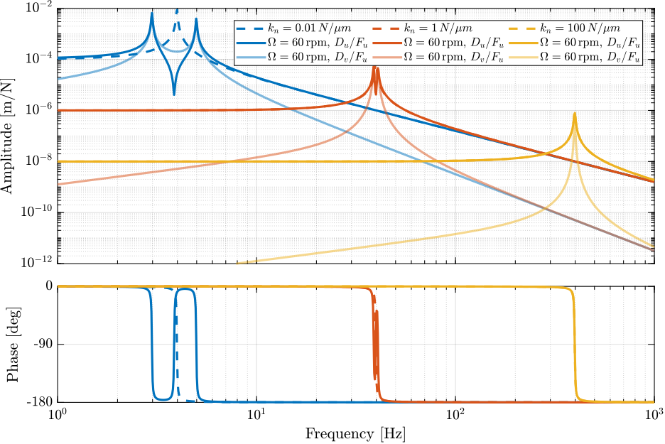

Effect of rotation on the nano-hexapod dynamics - Dashed lines are the plants without rotation, solid lines are plants at maximum rotating velocity, and shaded lines are coupling terms at maximum rotating velocity

Optimal IFF with High Pass Filter

Let's apply Integral Force Feedback with an added High Pass Filter to the three nano-hexapods.

First, let's find the parameters of the IFF controller that yield best simultaneous damping. The results are shown in Figure ref:fig:rotating_iff_hpf_nass_optimal_gain. The added damping for the soft nano-hexapod is quite low and is limited by the maximum usable gain.

%% Compute the optimal control gain
wis = logspace(-2, 3, 200); % [rad/s]

opt_iff_hpf_xi_vc = zeros(1, length(wis)); % Optimal simultaneous damping
opt_iff_hpf_gain_vc = zeros(1, length(wis)); % Corresponding optimal gain

opt_iff_hpf_xi_md = zeros(1, length(wis)); % Optimal simultaneous damping
opt_iff_hpf_gain_md = zeros(1, length(wis)); % Corresponding optimal gain

opt_iff_hpf_xi_pz = zeros(1, length(wis)); % Optimal simultaneous damping
opt_iff_hpf_gain_pz = zeros(1, length(wis)); % Corresponding optimal gain

for wi_i = 1:length(wis)
    wi = wis(wi_i);
    Kiff = 1/(s + wi)*eye(2);

    fun = @(g)computeSimultaneousDamping(g, G_vc_fast({'fu', 'fv'}, {'Fu', 'Fv'}), Kiff);

    [g_opt, xi_opt] = fminsearch(fun, 0.1);
    opt_iff_hpf_xi_vc(wi_i) = 1/xi_opt;
    opt_iff_hpf_gain_vc(wi_i) = g_opt;

    fun = @(g)computeSimultaneousDamping(g, G_md_fast({'fu', 'fv'}, {'Fu', 'Fv'}), Kiff);

    [g_opt, xi_opt] = fminsearch(fun, 0.1);
    opt_iff_hpf_xi_md(wi_i) = 1/xi_opt;
    opt_iff_hpf_gain_md(wi_i) = g_opt;

    fun = @(g)computeSimultaneousDamping(g, G_pz_fast({'fu', 'fv'}, {'Fu', 'Fv'}), Kiff);

    [g_opt, xi_opt] = fminsearch(fun, 0.1);
    opt_iff_hpf_xi_pz(wi_i) = 1/xi_opt;
    opt_iff_hpf_gain_pz(wi_i) = g_opt;
end

%% Optimal modified IFF parameters that yields maximum simultaneous damping
figure;
tiledlayout(1, 3, 'TileSpacing', 'Compact', 'Padding', 'None');

ax1 = nexttile();
yyaxis left
plot(wis, opt_iff_hpf_xi_vc, '-', 'DisplayName', '$\xi_{cl}$');
set(gca, 'YScale', 'lin');
ylim([0,1]);
ylabel('Damping Ratio $\xi$');

yyaxis right
hold on;
plot(wis, opt_iff_hpf_gain_vc, '-', 'DisplayName', '$g_{opt}$');
plot(wis, wis*((sqrt(1e4/16)/(2*pi))^2 - 1), '--', 'DisplayName', '$g_{max}$');
set(gca, 'YScale', 'lin');
ylim([0,200]);
xlabel('$\omega_i$ [rad/s]');
set(gca, 'YTickLabel',[]);
% ylabel('Controller gain $g$');
set(gca, 'XScale', 'log');
xticks([1e-2,1,1e2])
legend('location', 'northwest', 'FontSize', 8);
title('$k_n = 0.01\,N/\mu m$');

ax2 = nexttile();
yyaxis left
plot(wis, opt_iff_hpf_xi_md, '-');
set(gca, 'YScale', 'lin');
ylim([0,1]);
% ylabel('Damping Ratio $\xi$');
set(gca, 'YTickLabel',[]);

yyaxis right
hold on;
plot(wis, opt_iff_hpf_gain_md, '-');
plot(wis, wis*((sqrt(1e6/16)/(2*pi))^2 - 1), '--');
set(gca, 'YScale', 'lin');
ylim([0,1000]);
xlabel('$\omega_i$ [rad/s]');
% ylabel('Controller gain $g$');
set(gca, 'YTickLabel',[]);
set(gca, 'XScale', 'log');
xticks([1e-2,1,1e2])
title('$k_n = 1\,N/\mu m$');

ax3 = nexttile();
yyaxis left
plot(wis, opt_iff_hpf_xi_pz, '-');
set(gca, 'YScale', 'lin');
ylim([0,1]);
set(gca, 'YTickLabel',[]);
% ylabel('Damping Ratio $\xi$');

yyaxis right
hold on;
plot(wis, opt_iff_hpf_gain_pz, '-');
plot(wis, wis*((sqrt(1e8/16)/(2*pi))^2 - 1), '--');
set(gca, 'YScale', 'lin');
ylim([0,10000]);
xlabel('$\omega_i$ [rad/s]');
set(gca, 'YTickLabel',[]);
ylabel('Controller gain $g$');
set(gca, 'XScale', 'log');
xticks([1e-2,1,1e2])
title('$k_n = 100\,N/\mu m$');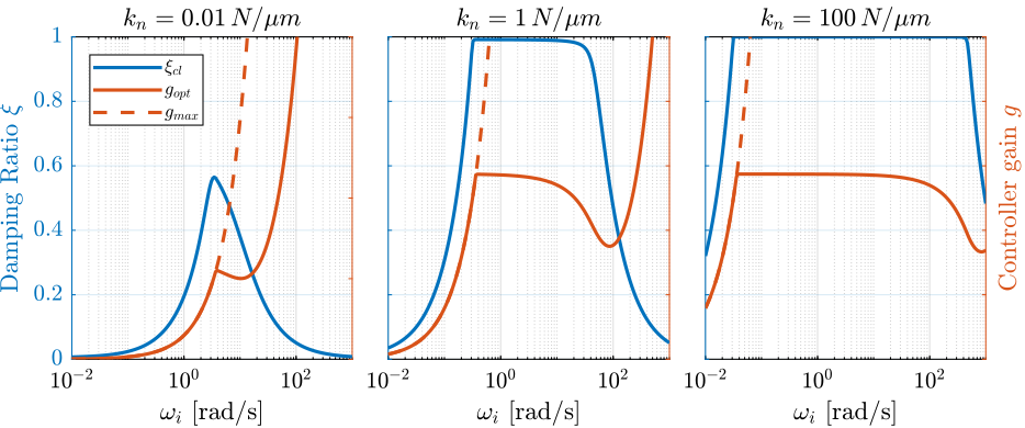

Optimal high pass filter cut-off frequency $\omega_i$ that yields maximum simultaneous damping

The IFF parameters are chosen as follow:

• for $k_n = \SI{0.01}{\N\per\mu\m}$: $\omega_i$ is chosen such that the maximum damping is achieved while the gain is less than half of the maximum gain at which the system is unstable. This is done to have some control robustness.
• for $k_n = \SI{1}{\N\per\mu\m}$ and $k_n = \SI{100}{\N\per\mu\m}$: the largest $\omega_i$ is chosen such that obtained damping is $\SI{95}{\percent}$ of the maximum achievable damping. Large $\omega_i$ is chosen here to limit the loss of compliance and the increase of coupling at low frequency as was shown in Section ref:sec:rotating_iff_pseudo_int.

The obtained IFF parameters and the achievable damping are summarized in Table ref:tab:iff_hpf_opt_iff_hpf_params_nass.

%% Find optimal parameters with at least a gain margin of 2
i_iff_hpf_vc = find(opt_iff_hpf_gain_vc < 0.5*(wis*((sqrt(1e4/16)/(2*pi))^2 - 1)));
i_iff_hpf_vc = i_iff_hpf_vc(1);

i_iff_hpf_md = find(opt_iff_hpf_xi_md > 0.95*max(opt_iff_hpf_xi_md));
i_iff_hpf_md = i_iff_hpf_md(end)+1;

i_iff_hpf_pz = find(opt_iff_hpf_xi_pz > 0.95*max(opt_iff_hpf_xi_pz));
i_iff_hpf_pz = i_iff_hpf_pz(end)+1;

	$\omega_i$	$g$	$\xi$
$k_n = 0.01\,N/\mu m$	7.32	51.13	0.45
$k_n = 1\,N/\mu m$	39.17	426.95	0.93
$k_n = 100\,N/\mu m$	499.45	3774.63	0.94

The Root Locus for all three nano-hexapods are shown in Figure ref:fig:rotating_root_locus_iff_hpf_nass with included optimal chosen gains.

%% Optimal IFF with added HPF
Kiff_hpf_vc = opt_iff_hpf_gain_vc(i_iff_hpf_vc)/(s + wis(i_iff_hpf_vc))*eye(2);
Kiff_hpf_vc.InputName = {'fu', 'fv'};
Kiff_hpf_vc.OutputName = {'Fu', 'Fv'};

Kiff_hpf_md = opt_iff_hpf_gain_md(i_iff_hpf_md)/(s + wis(i_iff_hpf_md))*eye(2);
Kiff_hpf_md.InputName = {'fu', 'fv'};
Kiff_hpf_md.OutputName = {'Fu', 'Fv'};

Kiff_hpf_pz = opt_iff_hpf_gain_pz(i_iff_hpf_pz)/(s + wis(i_iff_hpf_pz))*eye(2);
Kiff_hpf_pz.InputName = {'fu', 'fv'};
Kiff_hpf_pz.OutputName = {'Fu', 'Fv'};

%% Root Locus for optimal parameters - Comparison of attainable damping with the soft and moderately stiff nano-hexapods
gains = logspace(-2, 3, 200);

figure;
tiledlayout(1, 3, 'TileSpacing', 'Compact', 'Padding', 'None');

% Voice coil Nano-Hexapod
ax1 = nexttile();
hold on;
for g = gains
    clpoles = pole(feedback(G_vc_norot({'fu', 'fv'}, {'Fu', 'Fv'}), g*Kiff_hpf_vc));
    plot(real(clpoles), imag(clpoles), '.', 'color', colors(1,:),'MarkerSize',4, ...
        'HandleVisibility', 'off');
end
clpoles = pole(feedback(G_vc_norot({'fu', 'fv'}, {'Fu', 'Fv'}), Kiff_hpf_vc));
plot(real(clpoles), imag(clpoles), '.', 'color', colors(1,:),'MarkerSize', 15, ...
    'DisplayName', '$\Omega = 0$');
plot(real(pole(G_vc_norot({'fu', 'fv'}, {'Fu', 'Fv'})*Kiff_hpf_vc)), ...
     imag(pole(G_vc_norot({'fu', 'fv'}, {'Fu', 'Fv'})*Kiff_hpf_vc)), ...
     'x', 'color', colors(1,:),'MarkerSize',8, ...
        'HandleVisibility', 'off');
plot(real(tzero(G_vc_norot({'fu', 'fv'}, {'Fu', 'Fv'})*Kiff_hpf_vc)), ...
     imag(tzero(G_vc_norot({'fu', 'fv'}, {'Fu', 'Fv'})*Kiff_hpf_vc)), ...
     'o', 'color', colors(1,:),'MarkerSize',8, ...
        'HandleVisibility', 'off');

for g = gains
    clpoles = pole(feedback(G_vc_fast({'fu', 'fv'}, {'Fu', 'Fv'}), g*Kiff_hpf_vc));
    plot(real(clpoles), imag(clpoles), '.', 'color', colors(2,:),'MarkerSize',4, ...
        'HandleVisibility', 'off');
end
clpoles = pole(feedback(G_vc_fast({'fu', 'fv'}, {'Fu', 'Fv'}), Kiff_hpf_vc));
plot(real(clpoles), imag(clpoles), '.', 'color', colors(2,:),'MarkerSize', 15, ...
    'DisplayName', '$\Omega = 60$ rpm');
plot(real(pole(G_vc_fast({'fu', 'fv'}, {'Fu', 'Fv'})*Kiff_hpf_vc)), ...
     imag(pole(G_vc_fast({'fu', 'fv'}, {'Fu', 'Fv'})*Kiff_hpf_vc)), ...
     'x', 'color', colors(2,:),'MarkerSize',8, ...
        'HandleVisibility', 'off');
plot(real(tzero(G_vc_fast({'fu', 'fv'}, {'Fu', 'Fv'})*Kiff_hpf_vc)), ...
     imag(tzero(G_vc_fast({'fu', 'fv'}, {'Fu', 'Fv'})*Kiff_hpf_vc)), ...
     'o', 'color', colors(2,:),'MarkerSize',8, ...
        'HandleVisibility', 'off');

plot([0, -1e2*opt_iff_hpf_xi_vc(i_iff_hpf_vc)], [0, 1e2*cos(asin(opt_iff_hpf_xi_vc(i_iff_hpf_vc)))], '-', ...
     'DisplayName', sprintf('$\\xi = %.2f$', opt_iff_hpf_xi_vc(i_iff_hpf_vc)), 'color', [zeros(1,3), 0.5])
hold off;
axis square;
xlabel('Real Part'); ylabel('Imaginary Part');
xlim([-65, 5]); ylim([-35, 35]);
set(gca, 'XTickLabel',[]); set(gca, 'YTickLabel',[]);
title('$k_n = 0.01\,N/\mu m$');
ldg = legend('location', 'northwest', 'FontSize', 8, 'NumColumns', 1);
ldg.ItemTokenSize = [10, 1];

% APA Nano-Hexapod
ax2 = nexttile();
hold on;
for g = gains
    clpoles = pole(feedback(G_md_norot({'fu', 'fv'}, {'Fu', 'Fv'}), g*Kiff_hpf_md));
    plot(real(clpoles), imag(clpoles), '.', 'color', colors(1,:),'MarkerSize',4);
end
clpoles = pole(feedback(G_md_norot({'fu', 'fv'}, {'Fu', 'Fv'}), Kiff_hpf_md));
plot(real(clpoles), imag(clpoles), '.', 'color', colors(1,:),'MarkerSize', 15);
plot(real(pole(G_md_norot({'fu', 'fv'}, {'Fu', 'Fv'})*Kiff_hpf_md)), ...
     imag(pole(G_md_norot({'fu', 'fv'}, {'Fu', 'Fv'})*Kiff_hpf_md)), ...
     'x', 'color', colors(1,:),'MarkerSize',8);
plot(real(tzero(G_md_norot({'fu', 'fv'}, {'Fu', 'Fv'})*Kiff_hpf_md)), ...
     imag(tzero(G_md_norot({'fu', 'fv'}, {'Fu', 'Fv'})*Kiff_hpf_md)), ...
     'o', 'color', colors(1,:),'MarkerSize',8);

for g = gains
    clpoles = pole(feedback(G_md_fast({'fu', 'fv'}, {'Fu', 'Fv'}), g*Kiff_hpf_md));
    plot(real(clpoles), imag(clpoles), '.', 'color', colors(2,:),'MarkerSize',4);
end
clpoles = pole(feedback(G_md_fast({'fu', 'fv'}, {'Fu', 'Fv'}), Kiff_hpf_md));
plot(real(clpoles), imag(clpoles), '.', 'color', colors(2,:),'MarkerSize', 15);
plot(real(pole(G_md_fast({'fu', 'fv'}, {'Fu', 'Fv'})*Kiff_hpf_md)), ...
     imag(pole(G_md_fast({'fu', 'fv'}, {'Fu', 'Fv'})*Kiff_hpf_md)), ...
     'x', 'color', colors(2,:),'MarkerSize',8);
plot(real(tzero(G_md_fast({'fu', 'fv'}, {'Fu', 'Fv'})*Kiff_hpf_md)), ...
     imag(tzero(G_md_fast({'fu', 'fv'}, {'Fu', 'Fv'})*Kiff_hpf_md)), ...
     'o', 'color', colors(2,:),'MarkerSize',8);

L = plot([0, -1e3*opt_iff_hpf_xi_md(i_iff_hpf_md)], [0, 1e3*cos(asin(opt_iff_hpf_xi_md(i_iff_hpf_md)))], '-', ...
     'DisplayName', sprintf('$\\xi = %.2f$', opt_iff_hpf_xi_md(i_iff_hpf_md)), 'color', [zeros(1,3), 0.5]);
leg = legend(L, 'location', 'northwest', 'FontSize', 8);
leg.ItemTokenSize(1) = 10;
hold off;
axis square;
xlabel('Real Part'); ylabel('Imaginary Part');
xlim([-520, 20]); ylim([-270, 270]);
set(gca, 'XTickLabel',[]); set(gca, 'YTickLabel',[]);
title('$k_n = 1\,N/\mu m$');

% Piezo Nano-Hexapod
ax3 = nexttile();
hold on;
for g = gains
    clpoles = pole(feedback(G_pz_norot({'fu', 'fv'}, {'Fu', 'Fv'}), g*Kiff_hpf_pz));
    plot(real(clpoles), imag(clpoles), '.', 'color', colors(1,:),'MarkerSize',4);
end
clpoles = pole(feedback(G_pz_norot({'fu', 'fv'}, {'Fu', 'Fv'}), Kiff_hpf_pz));
plot(real(clpoles), imag(clpoles), '.', 'color', colors(1,:),'MarkerSize', 15);
plot(real(pole(G_pz_norot({'fu', 'fv'}, {'Fu', 'Fv'})*Kiff_hpf_pz)), ...
     imag(pole(G_pz_norot({'fu', 'fv'}, {'Fu', 'Fv'})*Kiff_hpf_pz)), ...
     'x', 'color', colors(1,:),'MarkerSize',8);
plot(real(tzero(G_pz_norot({'fu', 'fv'}, {'Fu', 'Fv'})*Kiff_hpf_pz)), ...
     imag(tzero(G_pz_norot({'fu', 'fv'}, {'Fu', 'Fv'})*Kiff_hpf_pz)), ...
     'o', 'color', colors(1,:),'MarkerSize',8);

for g = gains
    clpoles = pole(feedback(G_pz_fast({'fu', 'fv'}, {'Fu', 'Fv'}), g*Kiff_hpf_pz));
    plot(real(clpoles), imag(clpoles), '.', 'color', colors(2,:),'MarkerSize',4);
end
clpoles = pole(feedback(G_pz_fast({'fu', 'fv'}, {'Fu', 'Fv'}), Kiff_hpf_pz));
plot(real(clpoles), imag(clpoles), '.', 'color', colors(2,:),'MarkerSize', 15);
plot(real(pole(G_pz_fast({'fu', 'fv'}, {'Fu', 'Fv'})*Kiff_hpf_pz)), ...
     imag(pole(G_pz_fast({'fu', 'fv'}, {'Fu', 'Fv'})*Kiff_hpf_pz)), ...
     'x', 'color', colors(2,:),'MarkerSize',8);
plot(real(tzero(G_pz_fast({'fu', 'fv'}, {'Fu', 'Fv'})*Kiff_hpf_pz)), ...
     imag(tzero(G_pz_fast({'fu', 'fv'}, {'Fu', 'Fv'})*Kiff_hpf_pz)), ...
     'o', 'color', colors(2,:),'MarkerSize',8);

L = plot([0, -1e4*opt_iff_hpf_xi_pz(i_iff_hpf_pz)], [0, 1e4*cos(asin(opt_iff_hpf_xi_pz(i_iff_hpf_pz)))], '-', ...
     'DisplayName', sprintf('$\\xi = %.2f$', opt_iff_hpf_xi_pz(i_iff_hpf_pz)), 'color', [zeros(1,3), 0.5]);
leg = legend(L, 'location', 'northwest', 'FontSize', 8);
leg.ItemTokenSize(1) = 10;
hold off;
axis square;
xlabel('Real Part'); ylabel('Imaginary Part');
xlim([-5200, 20]); ylim([-2700, 2700]);
set(gca, 'XTickLabel',[]); set(gca, 'YTickLabel',[]);
title('$k_n = 100\,N/\mu m$');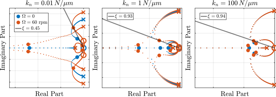

Root Locus for modified IFF with high pass filter. Optimal $\omega_i$ is used. The three nano-hexapod stiffnesses are compared. The grey line indicates the minimum damping obtained with the optimal chosen control parameters.

Optimal IFF with Parallel Stiffness

For each considered nano-hexapod stiffness, the parallel stiffness $k_p$ is varied from $k_{p,\text{min}} = m\Omega^2$ (the minimum stiffness to have unconditional stability) to $k_{p,\text{max}} = k_n$ (the total nano-hexapod stiffness). In order to keep the overall stiffness constant, the actuator stiffness $k_a$ is decreased when $k_p$ is increased:

\begin{equation} k_a = k_n - k_p \end{equation}

With $k_n$ the total nano-hexapod stiffness.

An high pass filter is also added to limit the low frequency gain. The cut-off frequency $\omega_i$ is chosen to be one tenth of the system resonance:

\begin{equation} \omega_i = \omega_0/10 \end{equation}

%% Maximum rotating velocity
Wz = 2*pi; % [rad/s]

%% Minimum parallel stiffness
kp_min = (mn + ms) * Wz^2; % [N/m]

%% Parameters for simulation
mn = 15; % Nano-Hexapod mass [kg]
ms = 1; % Sample Mass [kg]

%% IFF Controller
Kiff_vc = 1/(s + 0.1*sqrt(1e4/(mn+ms)))*eye(2); % IFF
Kiff_md = 1/(s + 0.1*sqrt(1e6/(mn+ms)))*eye(2); % IFF
Kiff_pz = 1/(s + 0.1*sqrt(1e8/(mn+ms)))*eye(2); % IFF

%% General Configuration
model_config = struct();
model_config.controller = "open_loop"; % Default: Open-Loop
model_config.Tuv_type   = "parallel_k";    % Default: 2DoF stage

%% Computes the optimal parameters and attainable simultaneous damping - Voice Coil nano-hexapod
kps_vc = logspace(log10(kp_min), log10(1e4), 100); % Tested parallel stiffnesses [N/m]
kps_vc(end) = [];

opt_iff_kp_xi_vc   = zeros(1, length(kps_vc)); % Optimal simultaneous damping
opt_iff_kp_gain_vc = zeros(1, length(kps_vc)); % Corresponding optimal gain

for kp_i = 1:length(kps_vc)
    % Voice Coil Nano-Hexapod
    kp = kps_vc(kp_i);
    cp = 2*0.001*sqrt((ms + mn)*kp);
    kn = 1e4 - kp; % Nano-Hexapod Stiffness [N/m]
    cn = 2*0.01*sqrt((ms + mn)*kn); % Nano-Hexapod Damping [N/(m/s)]

    % Identify dynamics
    Giff_vc = linearize(mdl, io, 0);
    Giff_vc.InputName  = {'Fu', 'Fv', 'Fdx', 'Fdy', 'Dfx', 'Dfy'};
    Giff_vc.OutputName = {'fu', 'fv', 'Du', 'Dv', 'Dx', 'Dy'};

    fun = @(g)computeSimultaneousDamping(g, Giff_vc({'fu', 'fv'}, {'Fu', 'Fv'}), Kiff_vc);

    [g_opt, xi_opt] = fminsearch(fun, 0.1);
    opt_iff_kp_xi_vc(kp_i) = 1/xi_opt;
    opt_iff_kp_gain_vc(kp_i) = g_opt;
end

%% Computes the optimal parameters and attainable simultaneous damping - APA nano-hexapod
kps_md = logspace(log10(kp_min), log10(1e6), 100); % Tested parallel stiffnesses [N/m]
kps_md(end) = [];

opt_iff_kp_xi_md   = zeros(1, length(kps_md)); % Optimal simultaneous damping
opt_iff_kp_gain_md = zeros(1, length(kps_md)); % Corresponding optimal gain


for kp_i = 1:length(kps_md)
    % Voice Coil Nano-Hexapod
    kp = kps_md(kp_i);
    cp = 2*0.001*sqrt((ms + mn)*kp);
    kn = 1e6 - kp; % Nano-Hexapod Stiffness [N/m]
    cn = 2*0.01*sqrt((ms + mn)*kn); % Nano-Hexapod Damping [N/(m/s)]

    % Identify dynamics
    Giff_md = linearize(mdl, io, 0);
    Giff_md.InputName  = {'Fu', 'Fv', 'Fdx', 'Fdy', 'Dfx', 'Dfy'};
    Giff_md.OutputName = {'fu', 'fv', 'Du', 'Dv', 'Dx', 'Dy'};

    fun = @(g)computeSimultaneousDamping(g, Giff_md({'fu', 'fv'}, {'Fu', 'Fv'}), Kiff_md);

    [g_opt, xi_opt] = fminsearch(fun, 0.1);
    opt_iff_kp_xi_md(kp_i) = 1/xi_opt;
    opt_iff_kp_gain_md(kp_i) = g_opt;
end

%% Computes the optimal parameters and attainable simultaneous damping - Piezo nano-hexapod
kps_pz = logspace(log10(kp_min), log10(1e8), 100); % Tested parallel stiffnesses [N/m]
kps_pz(end) = [];

opt_iff_kp_xi_pz   = zeros(1, length(kps_pz)); % Optimal simultaneous damping
opt_iff_kp_gain_pz = zeros(1, length(kps_pz)); % Corresponding optimal gain


for kp_i = 1:length(kps_pz)
    % Voice Coil Nano-Hexapod
    kp = kps_pz(kp_i);
    cp = 2*0.001*sqrt((ms + mn)*kp);
    kn = 1e8 - kp; % Nano-Hexapod Stiffness [N/m]
    cn = 2*0.01*sqrt((ms + mn)*kn); % Nano-Hexapod Damping [N/(m/s)]

    % Identify dynamics
    Giff_pz = linearize(mdl, io, 0);
    Giff_pz.InputName  = {'Fu', 'Fv', 'Fdx', 'Fdy', 'Dfx', 'Dfy'};
    Giff_pz.OutputName = {'fu', 'fv', 'Du', 'Dv', 'Dx', 'Dy'};

    fun = @(g)computeSimultaneousDamping(g, Giff_pz({'fu', 'fv'}, {'Fu', 'Fv'}), Kiff_pz);

    [g_opt, xi_opt] = fminsearch(fun, 0.1);
    opt_iff_kp_xi_pz(kp_i) = 1/xi_opt;
    opt_iff_kp_gain_pz(kp_i) = g_opt;
end

The achievable maximum simultaneous damping of all the modes is computed as a function of the parallel stiffnesses. The comparison for the nano-hexapod stiffnesses is done in Figure ref:fig:rotating_iff_kp_nass_optimal_gain. It is shown that the soft nano-hexapod cannot yield good damping. For the two stiff options, the achievable damping starts to significantly decrease when the parallel stiffness is one tenth of the total stiffness $k_p = k_n/10$.

%% Optimal IFF gain and associated simultaneous damping as a function of the parallel stiffness
figure;
hold on;
plot(kps_vc, opt_iff_kp_xi_vc, '-', 'DisplayName', '$k_n = 0.01\,N/\mu m$');
plot(kps_md, opt_iff_kp_xi_md, '-', 'DisplayName', '$k_n = 1\,N/\mu m$');
plot(kps_pz, opt_iff_kp_xi_pz, '-', 'DisplayName', '$k_n = 100\,N/\mu m$');
hold off;
xlabel('$k_p [N/m]$');
ylabel('Damping Ratio $\xi$');
set(gca, 'XScale', 'log');
set(gca, 'YScale', 'lin');
ylim([0,1]);
legend('location', 'southeast', 'FontSize', 8);
xlim([kps_pz(1), kps_pz(end)])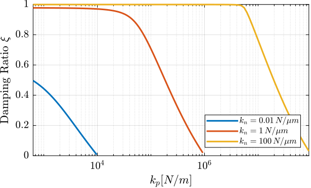

Maximum achievable simultaneous damping with IFF as a function of the parallel stiffness for all three nano-hexapod stiffnesses

Let's choose $k_p = \SI{e3}{\newton\per\m}$, $k_p = \SI{e4}{\newton\per\m}$ and $k_p = \SI{e6}{\newton\per\m}$ for the three considered nano-hexapods respectively based on Figure ref:fig:rotating_iff_kp_nass_optimal_gain.

The corresponding optimal controller gains are shown in Table ref:tab:iff_kp_opt_iff_kp_params_nass.

%% Find result with wanted parallel stiffness
[~, i_kp_vc] = min(abs(kps_vc - 1e3));
[~, i_kp_md] = min(abs(kps_md - 1e4));
[~, i_kp_pz] = min(abs(kps_pz - 1e6));

	$g$	$\xi_{\text{opt}}$
$k_n = 0.01\,N/\mu m$	47.9	0.44
$k_n = 1\,N/\mu m$	465.57	0.97
$k_n = 100\,N/\mu m$	4624.25	1.0

The root locus for the three nano-hexapod with parallel stiffnesses are shown in Figure ref:fig:rotating_root_locus_iff_kp_nass.

Similarly to what was found with the IFF and added High Pass Filter:

• the stiff nano-hexapod is less affected by the rotation than the soft one
• the achievable damping is much larger with the stiff nano-hexapods

%% Optimal IFF with added parallel stiffness
Kiff_kp_vc = opt_iff_kp_gain_vc(i_kp_vc)/(s + 0.1*sqrt(1e4/(ms+mn)))*eye(2);
Kiff_kp_vc.InputName = {'fu', 'fv'};
Kiff_kp_vc.OutputName = {'Fu', 'Fv'};

Kiff_kp_md = opt_iff_kp_gain_md(i_kp_md)/(s + 0.1*sqrt(1e6/(ms+mn)))*eye(2);
Kiff_kp_md.InputName = {'fu', 'fv'};
Kiff_kp_md.OutputName = {'Fu', 'Fv'};

Kiff_kp_pz = opt_iff_kp_gain_pz(i_kp_pz)/(s + 0.1*sqrt(1e8/(ms+mn)))*eye(2);
Kiff_kp_pz.InputName = {'fu', 'fv'};
Kiff_kp_pz.OutputName = {'Fu', 'Fv'};

%% Identify plant with optimal parallel stiffness - Soft nano-hexapod
kp = kps_vc(i_kp_vc);
cp = 2*0.001*sqrt((ms + mn)*kp);
kn = 1e4-kp; % Nano-Hexapod Stiffness [N/m]
cn = 2*0.01*sqrt((ms + mn)*kn); % Nano-Hexapod Damping [N/(m/s)]

% Identify dynamics
Wz = 2*pi; % [rad/s]
G_vc_kp_fast = linearize(mdl, io, 0);
G_vc_kp_fast.InputName  = {'Fu', 'Fv', 'Fdx', 'Fdy', 'Dfx', 'Dfy'};
G_vc_kp_fast.OutputName = {'fu', 'fv', 'Du', 'Dv', 'Dx', 'Dy'};

Wz = 0; % [rad/s]
G_vc_kp_norot = linearize(mdl, io, 0);
G_vc_kp_norot.InputName  = {'Fu', 'Fv', 'Fdx', 'Fdy', 'Dfx', 'Dfy'};
G_vc_kp_norot.OutputName = {'fu', 'fv', 'Du', 'Dv', 'Dx', 'Dy'};

%% Identify plant with optimal parallel stiffness - Stiff nano-hexapod
kp = kps_md(i_kp_md);
cp = 2*0.001*sqrt((ms + mn)*kp);
kn = 1e6 - kp; % Nano-Hexapod Stiffness [N/m]
cn = 2*0.01*sqrt((ms + mn)*kn); % Nano-Hexapod Damping [N/(m/s)]

% Identify dynamics
Wz = 2*pi; % [rad/s]
G_md_kp_fast = linearize(mdl, io, 0);
G_md_kp_fast.InputName  = {'Fu', 'Fv', 'Fdx', 'Fdy', 'Dfx', 'Dfy'};
G_md_kp_fast.OutputName = {'fu', 'fv', 'Du', 'Dv', 'Dx', 'Dy'};

Wz = 0; % [rad/s]
G_md_kp_norot = linearize(mdl, io, 0);
G_md_kp_norot.InputName  = {'Fu', 'Fv', 'Fdx', 'Fdy', 'Dfx', 'Dfy'};
G_md_kp_norot.OutputName = {'fu', 'fv', 'Du', 'Dv', 'Dx', 'Dy'};

%% Identify plant with optimal parallel stiffness - Stiff nano-hexapod
kp = kps_pz(i_kp_pz);
cp = 2*0.001*sqrt((ms + mn)*kp);
kn = 1e8 - kp; % Nano-Hexapod Stiffness [N/m]
cn = 2*0.01*sqrt((ms + mn)*kn); % Nano-Hexapod Damping [N/(m/s)]

% Identify dynamics
Wz = 2*pi; % [rad/s]
G_pz_kp_fast = linearize(mdl, io, 0);
G_pz_kp_fast.InputName  = {'Fu', 'Fv', 'Fdx', 'Fdy', 'Dfx', 'Dfy'};
G_pz_kp_fast.OutputName = {'fu', 'fv', 'Du', 'Dv', 'Dx', 'Dy'};

Wz = 0; % [rad/s]
G_pz_kp_norot = linearize(mdl, io, 0);
G_pz_kp_norot.InputName  = {'Fu', 'Fv', 'Fdx', 'Fdy', 'Dfx', 'Dfy'};
G_pz_kp_norot.OutputName = {'fu', 'fv', 'Du', 'Dv', 'Dx', 'Dy'};

%% Root Locus for optimal parameters - Comparison of attainable damping with the soft and moderately stiff nano-hexapods
gains = logspace(-2, 2, 400);

figure;
tiledlayout(1, 3, 'TileSpacing', 'Compact', 'Padding', 'None');

ax1 = nexttile();
hold on;
% Soft Nano-Hexapod - No Rotation
for g = gains
    clpoles = pole(feedback(G_vc_kp_norot({'fu', 'fv'}, {'Fu', 'Fv'}), g*Kiff_kp_vc));
    plot(real(clpoles), imag(clpoles), '.', 'color', colors(1,:),'MarkerSize',4, ...
        'HandleVisibility', 'off');
end
clpoles = pole(feedback(G_vc_kp_norot({'fu', 'fv'}, {'Fu', 'Fv'}), Kiff_kp_vc));
plot(real(clpoles), imag(clpoles), '.', 'color', colors(1,:),'MarkerSize', 15, ...
    'DisplayName', '$\Omega = 0$');
plot(real(pole(G_vc_kp_norot({'fu', 'fv'}, {'Fu', 'Fv'})*Kiff_kp_vc)), ...
     imag(pole(G_vc_kp_norot({'fu', 'fv'}, {'Fu', 'Fv'})*Kiff_kp_vc)), ...
     'x', 'color', colors(1,:),'MarkerSize',8, ...
        'HandleVisibility', 'off');
plot(real(tzero(G_vc_kp_norot({'fu', 'fv'}, {'Fu', 'Fv'})*Kiff_kp_vc)), ...
     imag(tzero(G_vc_kp_norot({'fu', 'fv'}, {'Fu', 'Fv'})*Kiff_kp_vc)), ...
     'o', 'color', colors(1,:),'MarkerSize',8, ...
        'HandleVisibility', 'off');

% Soft Nano-Hexapod - High Speed Rotation
for g = gains
    clpoles = pole(feedback(G_vc_kp_fast({'fu', 'fv'}, {'Fu', 'Fv'}), g*Kiff_kp_vc));
    plot(real(clpoles), imag(clpoles), '.', 'color', colors(2,:),'MarkerSize',4, ...
        'HandleVisibility', 'off');
end
clpoles = pole(feedback(G_vc_kp_fast({'fu', 'fv'}, {'Fu', 'Fv'}), Kiff_kp_vc));
plot(real(clpoles), imag(clpoles), '.', 'color', colors(2,:),'MarkerSize', 15, ...
    'DisplayName', '$\Omega = 60$ rpm');
plot(real(pole(G_vc_kp_fast({'fu', 'fv'}, {'Fu', 'Fv'})*Kiff_kp_vc)), ...
     imag(pole(G_vc_kp_fast({'fu', 'fv'}, {'Fu', 'Fv'})*Kiff_kp_vc)), ...
     'x', 'color', colors(2,:),'MarkerSize',8, ...
        'HandleVisibility', 'off');
plot(real(tzero(G_vc_kp_fast({'fu', 'fv'}, {'Fu', 'Fv'})*Kiff_kp_vc)), ...
     imag(tzero(G_vc_kp_fast({'fu', 'fv'}, {'Fu', 'Fv'})*Kiff_kp_vc)), ...
     'o', 'color', colors(2,:),'MarkerSize',8, ...
        'HandleVisibility', 'off');
plot([0, -1e2*opt_iff_kp_xi_vc(i_kp_vc)], [0, 1e2*cos(asin(opt_iff_kp_xi_vc(i_kp_vc)))], '-', ...
     'DisplayName', sprintf('$\\xi = %.2f$', opt_iff_kp_xi_vc(i_kp_vc)), 'color', [zeros(1,3), 0.5]);
hold off;
axis square;
xlabel('Real Part'); ylabel('Imaginary Part');
xlim([-65, 5]); ylim([-35, 35]);
set(gca, 'XTickLabel',[]); set(gca, 'YTickLabel',[]);
title('$k_n = 0.01\,N/\mu m$');
ldg = legend('location', 'northwest', 'FontSize', 8, 'NumColumns', 1);
ldg.ItemTokenSize = [10, 1];

ax2 = nexttile();
hold on;
% Stiff Nano-Hexapod - No Rotation
for g = gains
    clpoles = pole(feedback(G_md_kp_norot({'fu', 'fv'}, {'Fu', 'Fv'}), g*Kiff_kp_md));
    plot(real(clpoles), imag(clpoles), '.', 'color', colors(1,:),'MarkerSize',4);
end
clpoles = pole(feedback(G_md_kp_norot({'fu', 'fv'}, {'Fu', 'Fv'}), Kiff_kp_md));
plot(real(clpoles), imag(clpoles), '.', 'color', colors(1,:),'MarkerSize', 15);
plot(real(pole(G_md_kp_norot({'fu', 'fv'}, {'Fu', 'Fv'})*Kiff_kp_md)), ...
     imag(pole(G_md_kp_norot({'fu', 'fv'}, {'Fu', 'Fv'})*Kiff_kp_md)), ...
     'x', 'color', colors(1,:),'MarkerSize',8);
plot(real(tzero(G_md_kp_norot({'fu', 'fv'}, {'Fu', 'Fv'})*Kiff_kp_md)), ...
     imag(tzero(G_md_kp_norot({'fu', 'fv'}, {'Fu', 'Fv'})*Kiff_kp_md)), ...
     'o', 'color', colors(1,:),'MarkerSize',8);

% Stiff Nano-Hexapod - High Speed Rotation
for g = gains
    clpoles = pole(feedback(G_md_kp_fast({'fu', 'fv'}, {'Fu', 'Fv'}), g*Kiff_kp_md));
    plot(real(clpoles), imag(clpoles), '.', 'color', colors(2,:),'MarkerSize',4);
end
clpoles = pole(feedback(G_md_kp_fast({'fu', 'fv'}, {'Fu', 'Fv'}), Kiff_kp_md));
plot(real(clpoles), imag(clpoles), '.', 'color', colors(2,:),'MarkerSize', 15);
plot(real(pole(G_md_kp_fast({'fu', 'fv'}, {'Fu', 'Fv'})*Kiff_kp_md)), ...
     imag(pole(G_md_kp_fast({'fu', 'fv'}, {'Fu', 'Fv'})*Kiff_kp_md)), ...
     'x', 'color', colors(2,:),'MarkerSize',8);
plot(real(tzero(G_md_kp_fast({'fu', 'fv'}, {'Fu', 'Fv'})*Kiff_kp_md)), ...
     imag(tzero(G_md_kp_fast({'fu', 'fv'}, {'Fu', 'Fv'})*Kiff_kp_md)), ...
     'o', 'color', colors(2,:),'MarkerSize',8);
L = plot([0, -1e3*opt_iff_kp_xi_md(i_kp_md)], [0, 1e3*cos(asin(opt_iff_kp_xi_md(i_kp_md)))], '-', ...
     'DisplayName', sprintf('$\\xi = %.2f$', opt_iff_kp_xi_md(i_kp_md)), 'color', [zeros(1,3), 0.5]);
leg = legend(L, 'location', 'northwest', 'FontSize', 8);
leg.ItemTokenSize(1) = 10;
hold off;
axis square;
xlabel('Real Part'); ylabel('Imaginary Part');
set(gca, 'XTickLabel',[]); set(gca, 'YTickLabel',[]);
xlim([-520, 20]); ylim([-270, 270]);
title('$k_n = 1\,N/\mu m$');

ax3 = nexttile();
hold on;
% Stiff Nano-Hexapod - No Rotation
for g = gains
    clpoles = pole(feedback(G_pz_kp_norot({'fu', 'fv'}, {'Fu', 'Fv'}), g*Kiff_kp_pz));
    plot(real(clpoles), imag(clpoles), '.', 'color', colors(1,:),'MarkerSize',4);
end
clpoles = pole(feedback(G_pz_kp_norot({'fu', 'fv'}, {'Fu', 'Fv'}), Kiff_kp_pz));
plot(real(clpoles), imag(clpoles), '.', 'color', colors(1,:),'MarkerSize', 15);
plot(real(pole(G_pz_kp_norot({'fu', 'fv'}, {'Fu', 'Fv'})*Kiff_kp_pz)), ...
     imag(pole(G_pz_kp_norot({'fu', 'fv'}, {'Fu', 'Fv'})*Kiff_kp_pz)), ...
     'x', 'color', colors(1,:),'MarkerSize',8);
plot(real(tzero(G_pz_kp_norot({'fu', 'fv'}, {'Fu', 'Fv'})*Kiff_kp_pz)), ...
     imag(tzero(G_pz_kp_norot({'fu', 'fv'}, {'Fu', 'Fv'})*Kiff_kp_pz)), ...
     'o', 'color', colors(1,:),'MarkerSize',8);

% Stiff Nano-Hexapod - High Speed Rotation
for g = gains
    clpoles = pole(feedback(G_pz_kp_fast({'fu', 'fv'}, {'Fu', 'Fv'}), g*Kiff_kp_pz));
    plot(real(clpoles), imag(clpoles), '.', 'color', colors(2,:),'MarkerSize',4);
end
clpoles = pole(feedback(G_pz_kp_fast({'fu', 'fv'}, {'Fu', 'Fv'}), Kiff_kp_pz));
plot(real(clpoles), imag(clpoles), '.', 'color', colors(2,:),'MarkerSize', 15);
plot(real(pole(G_pz_kp_fast({'fu', 'fv'}, {'Fu', 'Fv'})*Kiff_kp_pz)), ...
     imag(pole(G_pz_kp_fast({'fu', 'fv'}, {'Fu', 'Fv'})*Kiff_kp_pz)), ...
     'x', 'color', colors(2,:),'MarkerSize',8);
plot(real(tzero(G_pz_kp_fast({'fu', 'fv'}, {'Fu', 'Fv'})*Kiff_kp_pz)), ...
     imag(tzero(G_pz_kp_fast({'fu', 'fv'}, {'Fu', 'Fv'})*Kiff_kp_pz)), ...
     'o', 'color', colors(2,:),'MarkerSize',8);
L = plot([0, -1e4*opt_iff_kp_xi_pz(i_kp_pz)], [0, 1e4*cos(asin(opt_iff_kp_xi_pz(i_kp_pz)))], '-', ...
     'DisplayName', sprintf('$\\xi = %.2f$', opt_iff_kp_xi_pz(i_kp_pz)), 'color', [zeros(1,3), 0.5]);
leg = legend(L, 'location', 'northwest', 'FontSize', 8);
leg.ItemTokenSize(1) = 10;
hold off;
axis square;
xlabel('Real Part'); ylabel('Imaginary Part');
set(gca, 'XTickLabel',[]); set(gca, 'YTickLabel',[]);
xlim([-5200, 200]); ylim([-2700, 2700]);
title('$k_n = 100\,N/\mu m$');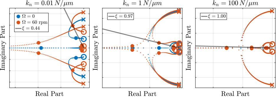

Root Locus for optimal parameters (IFF + $k_p$ strategy) - Comparison of attainable damping with the three nano-hexapod stiffnesses

Optimal Relative Motion Control

For each considered nano-hexapod stiffness, relative damping control is applied and the achievable damping ratio as a function of the controller gain is shown in Figure ref:fig:rotating_rdc_optimal_gain.

%% Computes the optimal parameters and attainable simultaneous damping - Piezo nano-hexapod
rdc_gains = 2*logspace(1, 5, 200);
% Obtained simultaneous damping
rdc_xi_vc = zeros(1, length(rdc_gains));
rdc_xi_md = zeros(1, length(rdc_gains));
rdc_xi_pz = zeros(1, length(rdc_gains));

Krdc = s*eye(2);
Krdc.InputName  = {'Du', 'Dv'};
Krdc.OutputName = {'Fu', 'Fv'};

for g_i = 1:length(rdc_gains)
    [~, xi] = damp(feedback(G_vc_fast({'Du', 'Dv'}, {'Fu', 'Fv'}), rdc_gains(g_i)*Krdc));
    rdc_xi_vc(g_i) = min(xi);

    [~, xi] = damp(feedback(G_md_fast({'Du', 'Dv'}, {'Fu', 'Fv'}), rdc_gains(g_i)*Krdc));
    rdc_xi_md(g_i) = min(xi);

    [~, xi] = damp(feedback(G_pz_fast({'Du', 'Dv'}, {'Fu', 'Fv'}), rdc_gains(g_i)*Krdc));
    rdc_xi_pz(g_i) = min(xi);
end

%% Optimal IFF gain and associated simultaneous damping as a function of the parallel stiffness
figure;
hold on;
plot(rdc_gains, rdc_xi_vc, '-', 'DisplayName', '$k_n = 0.01\,N/\mu m$');
plot(rdc_gains, rdc_xi_md, '-', 'DisplayName', '$k_n = 1\,N/\mu m$');
plot(rdc_gains, rdc_xi_pz, '-', 'DisplayName', '$k_n = 100\,N/\mu m$');
hold off;
xlabel('Relative Damping Controller gain $g$');
ylabel('Damping Ratio $\xi$');
set(gca, 'XScale', 'log');
set(gca, 'YScale', 'lin');
ylim([0,1]);
xlim([rdc_gains(1), rdc_gains(end)])
legend('location', 'southeast', 'FontSize', 8);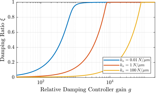

Achievable simultaneous damping with "Relative Damping Control" as a function of the controller gain for all three nano-hexapod stiffnesses

The gain is chosen is chosen such that 99% of modal damping is obtained. The root locus for all three nano-hexapod stiffnesses are shown in Figure ref:fig:rotating_root_locus_rdc_nass.

Relative damping control is much less impacted by gyroscopic effects. It can be easily applied on the nano-hexapod with and without rotation without much differences.

%% Optimal RDC
[~, i_rdc_vc] = min(abs(rdc_xi_vc - 0.99));
[~, i_rdc_md] = min(abs(rdc_xi_md - 0.99));
[~, i_rdc_pz] = min(abs(rdc_xi_pz - 0.99));

Krdc_vc = rdc_gains(i_rdc_vc)*Krdc;
Krdc_md = rdc_gains(i_rdc_md)*Krdc;
Krdc_pz = rdc_gains(i_rdc_pz)*Krdc;

%% Root Locus for optimal parameters - Comparison of attainable damping with the soft and moderately strdc nano-hexapods
gains = logspace(-2, 3, 200);

figure;
tiledlayout(1, 3, 'TileSpacing', 'Compact', 'Padding', 'None');

% Voice coil Nano-Hexapod
ax1 = nexttile();
hold on;
for g = gains
    clpoles = pole(feedback(G_vc_norot({'Du', 'Dv'}, {'Fu', 'Fv'}), g*Krdc_vc));
    plot(real(clpoles), imag(clpoles), '.', 'color', colors(1,:),'MarkerSize',4, ...
         'HandleVisibility', 'off');
end
clpoles = pole(feedback(G_vc_norot({'Du', 'Dv'}, {'Fu', 'Fv'}), Krdc_vc));
plot(real(clpoles), imag(clpoles), '.', 'color', colors(1,:),'MarkerSize', 15, ...
     'DisplayName', '$\Omega = 0$');
plot(real(pole(G_vc_norot({'Du', 'Dv'}, {'Fu', 'Fv'})*Krdc_vc)), ...
     imag(pole(G_vc_norot({'Du', 'Dv'}, {'Fu', 'Fv'})*Krdc_vc)), ...
     'x', 'color', colors(1,:),'MarkerSize',8, ...
     'HandleVisibility', 'off');
plot(real(tzero(G_vc_norot({'Du', 'Dv'}, {'Fu', 'Fv'})*Krdc_vc)), ...
     imag(tzero(G_vc_norot({'Du', 'Dv'}, {'Fu', 'Fv'})*Krdc_vc)), ...
     'o', 'color', colors(1,:),'MarkerSize',8, ...
     'HandleVisibility', 'off');

for g = gains
    clpoles = pole(feedback(G_vc_fast({'Du', 'Dv'}, {'Fu', 'Fv'}), g*Krdc_vc));
    plot(real(clpoles), imag(clpoles), '.', 'color', colors(2,:),'MarkerSize',4, ...
         'HandleVisibility', 'off');
end
clpoles = pole(feedback(G_vc_fast({'Du', 'Dv'}, {'Fu', 'Fv'}), Krdc_vc));
plot(real(clpoles), imag(clpoles), '.', 'color', colors(2,:),'MarkerSize', 15, ...
     'DisplayName', '$\Omega = 60$ rpm');
plot(real(pole(G_vc_fast({'Du', 'Dv'}, {'Fu', 'Fv'})*Krdc_vc)), ...
     imag(pole(G_vc_fast({'Du', 'Dv'}, {'Fu', 'Fv'})*Krdc_vc)), ...
     'x', 'color', colors(2,:),'MarkerSize',8, ...
     'HandleVisibility', 'off');
plot(real(tzero(G_vc_fast({'Du', 'Dv'}, {'Fu', 'Fv'})*Krdc_vc)), ...
     imag(tzero(G_vc_fast({'Du', 'Dv'}, {'Fu', 'Fv'})*Krdc_vc)), ...
     'o', 'color', colors(2,:),'MarkerSize',8, ...
     'HandleVisibility', 'off');

plot([0, -1e2*rdc_xi_vc(i_rdc_vc)], [0, 1e2*cos(asin(rdc_xi_vc(i_rdc_vc)))], '-', ...
     'DisplayName', sprintf('$\\xi = %.2f$', rdc_xi_vc(i_rdc_vc)), 'color', [zeros(1,3), 0.5])
hold off;
axis square;
xlabel('Real Part'); ylabel('Imaginary Part');
xlim([-65, 5]); ylim([-35, 35]);
set(gca, 'XTickLabel',[]); set(gca, 'YTickLabel',[]);
title('$k_n = 0.01\,N/\mu m$');
ldg = legend('location', 'northwest', 'FontSize', 8, 'NumColumns', 1);
ldg.ItemTokenSize = [10, 1];

% APA Nano-Hexapod
ax2 = nexttile();
hold on;
for g = gains
    clpoles = pole(feedback(G_md_norot({'Du', 'Dv'}, {'Fu', 'Fv'}), g*Krdc_md));
    plot(real(clpoles), imag(clpoles), '.', 'color', colors(1,:),'MarkerSize',4);
end
clpoles = pole(feedback(G_md_norot({'Du', 'Dv'}, {'Fu', 'Fv'}), Krdc_md));
plot(real(clpoles), imag(clpoles), '.', 'color', colors(1,:),'MarkerSize', 15);
plot(real(pole(G_md_norot({'Du', 'Dv'}, {'Fu', 'Fv'})*Krdc_md)), ...
     imag(pole(G_md_norot({'Du', 'Dv'}, {'Fu', 'Fv'})*Krdc_md)), ...
     'x', 'color', colors(1,:),'MarkerSize',8);
plot(real(tzero(G_md_norot({'Du', 'Dv'}, {'Fu', 'Fv'})*Krdc_md)), ...
     imag(tzero(G_md_norot({'Du', 'Dv'}, {'Fu', 'Fv'})*Krdc_md)), ...
     'o', 'color', colors(1,:),'MarkerSize',8);

for g = gains
    clpoles = pole(feedback(G_md_fast({'Du', 'Dv'}, {'Fu', 'Fv'}), g*Krdc_md));
    plot(real(clpoles), imag(clpoles), '.', 'color', colors(2,:),'MarkerSize',4);
end
clpoles = pole(feedback(G_md_fast({'Du', 'Dv'}, {'Fu', 'Fv'}), Krdc_md));
plot(real(clpoles), imag(clpoles), '.', 'color', colors(2,:),'MarkerSize', 15);
plot(real(pole(G_md_fast({'Du', 'Dv'}, {'Fu', 'Fv'})*Krdc_md)), ...
     imag(pole(G_md_fast({'Du', 'Dv'}, {'Fu', 'Fv'})*Krdc_md)), ...
     'x', 'color', colors(2,:),'MarkerSize',8);
plot(real(tzero(G_md_fast({'Du', 'Dv'}, {'Fu', 'Fv'})*Krdc_md)), ...
     imag(tzero(G_md_fast({'Du', 'Dv'}, {'Fu', 'Fv'})*Krdc_md)), ...
     'o', 'color', colors(2,:),'MarkerSize',8);

L = plot([0, -1e3*rdc_xi_md(i_rdc_md)], [0, 1e3*cos(asin(rdc_xi_md(i_rdc_md)))], '-', ...
         'DisplayName', sprintf('$\\xi = %.2f$', rdc_xi_md(i_rdc_md)), 'color', [zeros(1,3), 0.5]);
leg = legend(L, 'location', 'northwest', 'FontSize', 8);
leg.ItemTokenSize(1) = 10;
hold off;
axis square;
xlabel('Real Part'); ylabel('Imaginary Part');
xlim([-520, 20]); ylim([-270, 270]);
set(gca, 'XTickLabel',[]); set(gca, 'YTickLabel',[]);
title('$k_n = 1\,N/\mu m$');

% Piezo Nano-Hexapod
ax3 = nexttile();
hold on;
for g = gains
    clpoles = pole(feedback(G_pz_norot({'Du', 'Dv'}, {'Fu', 'Fv'}), g*Krdc_pz));
    plot(real(clpoles), imag(clpoles), '.', 'color', colors(1,:),'MarkerSize',4);
end
clpoles = pole(feedback(G_pz_norot({'Du', 'Dv'}, {'Fu', 'Fv'}), Krdc_pz));
plot(real(clpoles), imag(clpoles), '.', 'color', colors(1,:),'MarkerSize', 15);
plot(real(pole(G_pz_norot({'Du', 'Dv'}, {'Fu', 'Fv'})*Krdc_pz)), ...
     imag(pole(G_pz_norot({'Du', 'Dv'}, {'Fu', 'Fv'})*Krdc_pz)), ...
     'x', 'color', colors(1,:),'MarkerSize',8);
plot(real(tzero(G_pz_norot({'Du', 'Dv'}, {'Fu', 'Fv'})*Krdc_pz)), ...
     imag(tzero(G_pz_norot({'Du', 'Dv'}, {'Fu', 'Fv'})*Krdc_pz)), ...
     'o', 'color', colors(1,:),'MarkerSize',8);

for g = gains
    clpoles = pole(feedback(G_pz_fast({'Du', 'Dv'}, {'Fu', 'Fv'}), g*Krdc_pz));
    plot(real(clpoles), imag(clpoles), '.', 'color', colors(2,:),'MarkerSize',4);
end
clpoles = pole(feedback(G_pz_fast({'Du', 'Dv'}, {'Fu', 'Fv'}), Krdc_pz));
plot(real(clpoles), imag(clpoles), '.', 'color', colors(2,:),'MarkerSize', 15);
plot(real(pole(G_pz_fast({'Du', 'Dv'}, {'Fu', 'Fv'})*Krdc_pz)), ...
     imag(pole(G_pz_fast({'Du', 'Dv'}, {'Fu', 'Fv'})*Krdc_pz)), ...
     'x', 'color', colors(2,:),'MarkerSize',8);
plot(real(tzero(G_pz_fast({'Du', 'Dv'}, {'Fu', 'Fv'})*Krdc_pz)), ...
     imag(tzero(G_pz_fast({'Du', 'Dv'}, {'Fu', 'Fv'})*Krdc_pz)), ...
     'o', 'color', colors(2,:),'MarkerSize',8);

L = plot([0, -1e4*rdc_xi_pz(i_rdc_pz)], [0, 1e4*cos(asin(rdc_xi_pz(i_rdc_pz)))], '-', ...
         'DisplayName', sprintf('$\\xi = %.2f$', rdc_xi_pz(i_rdc_pz)), 'color', [zeros(1,3), 0.5]);
leg = legend(L, 'location', 'northwest', 'FontSize', 8);
leg.ItemTokenSize(1) = 10;
hold off;
axis square;
xlabel('Real Part'); ylabel('Imaginary Part');
xlim([-5200, 20]); ylim([-2700, 2700]);
set(gca, 'XTickLabel',[]); set(gca, 'YTickLabel',[]);
title('$k_n = 100\,N/\mu m$');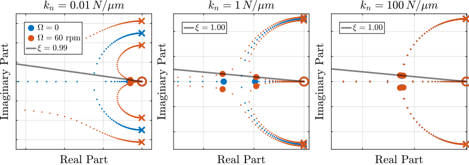

Root Locus for optimal parameters - Comparison of attainable damping with the soft and moderately stiff nano-hexapods

Comparison of the obtained damped plants

Let's now compare the obtained damped plants for the three active damping techniques applied on the three nano-hexapod stiffnesses (Figure ref:fig:rotating_nass_damped_plant_comp).

Similarly to what was concluded in previous analysis:

• IFF adds coupling below the resonance frequency as compared to the open-loop and RDC cases
• Add three methods are yielding good damping, except for IFF applied on the soft nano-hexapod where things are more complicated
• Coupling is smaller for stiff nano-hexapods

%% Saved controllers
save('./matlab/mat/nass_controllers.mat', ...
     'Kiff_hpf_vc', 'Kiff_hpf_md', 'Kiff_hpf_pz', ...
     'Kiff_kp_vc', 'Kiff_kp_md', 'Kiff_kp_pz', ...
     'Krdc_vc', 'Krdc_md', 'Krdc_pz');

%% Load controllers
load('nass_controllers.mat');

%% Closed Loop Plants - IFF with HPF
G_vc_norot_iff_hpf = feedback(G_vc_norot, Kiff_hpf_vc, 'name');
G_vc_fast_iff_hpf  = feedback(G_vc_fast,  Kiff_hpf_vc, 'name');

G_md_norot_iff_hpf = feedback(G_md_norot, Kiff_hpf_md, 'name');
G_md_fast_iff_hpf  = feedback(G_md_fast,  Kiff_hpf_md, 'name');

G_pz_norot_iff_hpf = feedback(G_pz_norot, Kiff_hpf_pz, 'name');
G_pz_fast_iff_hpf  = feedback(G_pz_fast,  Kiff_hpf_pz, 'name');

%% Closed Loop Plants - IFF with Parallel Stiffness
G_vc_norot_iff_kp = feedback(G_vc_kp_norot, Kiff_kp_vc, 'name');
G_vc_fast_iff_kp  = feedback(G_vc_kp_fast,  Kiff_kp_vc, 'name');

G_md_norot_iff_kp = feedback(G_md_kp_norot, Kiff_kp_md, 'name');
G_md_fast_iff_kp  = feedback(G_md_kp_fast,  Kiff_kp_md, 'name');

G_pz_norot_iff_kp = feedback(G_pz_kp_norot, Kiff_kp_pz, 'name');
G_pz_fast_iff_kp  = feedback(G_pz_kp_fast,  Kiff_kp_pz, 'name');

%% Closed Loop Plants - RDC
G_vc_norot_rdc = feedback(G_vc_norot, Krdc_vc, 'name');
G_vc_fast_rdc  = feedback(G_vc_fast,  Krdc_vc, 'name');

G_md_norot_rdc = feedback(G_md_norot, Krdc_md, 'name');
G_md_fast_rdc  = feedback(G_md_fast,  Krdc_md, 'name');

G_pz_norot_rdc = feedback(G_pz_norot, Krdc_pz, 'name');
G_pz_fast_rdc  = feedback(G_pz_fast,  Krdc_pz, 'name');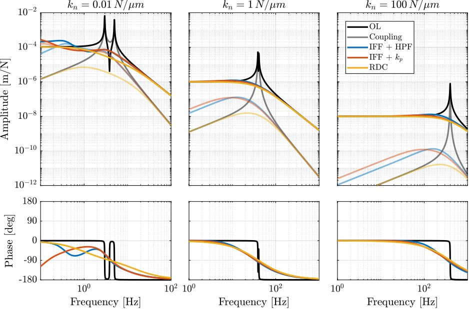

Comparison of the damped plants (direct and coupling terms) for the three proposed active damping techniques (IFF with HPF, IFF with $k_p$ and RDC) applied on the three nano-hexapod stiffnesses. $\Omega = 60\,\text{rmp}$ and $m_n + m_s = \SI{16}{\kg}$.

Nano-Active-Stabilization-System with rotation

<<sec:rotating_nass>>

Introduction   ignore

Up until now, the model used consisted of an infinitely stiff vertical rotating stage with a X-Y suspended stage.

While quite simplistic, this allowed to study the effects of rotation and the associated limitations when active damping is to be applied.

In this section, the limited compliance of the micro-station is taken into account as well as the rotation of the spindle.

NASS model

In order to be a bit closer to the NASS application, the 2DoF nano-hexapod (modelled as shown in Figure ref:fig:rotating_3dof_model_schematic) is now located on top of a model of the micro-station including (see Figure ref:fig:rotating_nass_model for a 3D view):

• the floor whose motion is imposed
• a 2DoF granite ($k_{g,x} = k_{g,y} = \SI{950}{\N\per\mu\m}$, $m_g = \SI{2500}{\kg}$)
• a 2DoF $T_y$ stage ($k_{t,x} = k_{t,y} = \SI{520}{\N\per\mu\m}$, $m_g = \SI{600}{\kg}$)
• a spindle (vertical rotation) stage whose rotation is imposed ($m_s = \SI{600}{\kg}$)
• a 2DoF micro-hexapod ($k_{h,x} = k_{h,y} = \SI{61}{\N\per\mu\m}$, $m_g = \SI{15}{\kg}$)

A payload is rigidly fixed to the nano-hexapod and the $x,y$ motion of the payload is measured with respect to the granite.

3D view of the Nano-Active-Stabilization-System model.

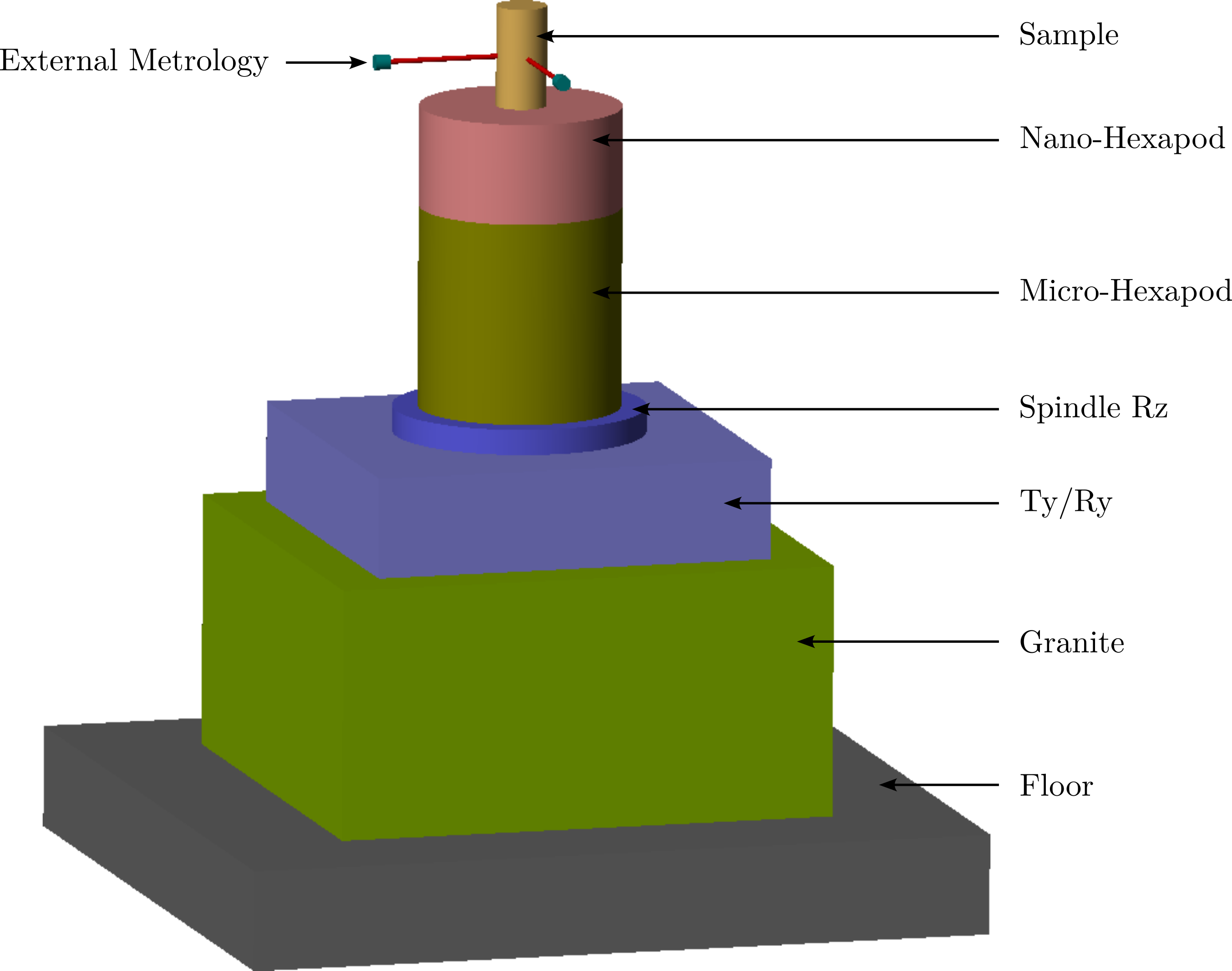
System dynamics

%% Nano-Hexapod
mn = 15; % Nano-Hexapod mass [kg]

%% Light Sample
ms = 1; % Sample Mass [kg]

%% General Configuration
model_config = struct();
model_config.controller = "open_loop"; % Default: Open-Loop
model_config.Tuv_type   = "normal";    % Default: 2DoF stage

%% Input/Output definition
clear io; io_i = 1;
io(io_i) = linio([mdl, '/controller'],   1, 'openinput');  io_i = io_i + 1; % Actuator Forces [Fu, Fv]
io(io_i) = linio([mdl, '/fd'],           1, 'openinput');  io_i = io_i + 1; % Direct Forces on Sample [Fdx, Fdy]
io(io_i) = linio([mdl, '/xf'],           1, 'openinput');  io_i = io_i + 1; % Floor Motion [Dfx, Dfy]
io(io_i) = linio([mdl, '/ft'],           1, 'openinput');  io_i = io_i + 1; % Micro-Station Disturbances [Ftx, Fty]
io(io_i) = linio([mdl, '/nano_hexapod'], 1, 'openoutput'); io_i = io_i + 1; % [Fmu, Fmv]
io(io_i) = linio([mdl, '/nano_hexapod'], 2, 'openoutput'); io_i = io_i + 1; % [Du, Dv]
io(io_i) = linio([mdl, '/ext_metrology'],1, 'openoutput'); io_i = io_i + 1; % [Dx, Dy]

The dynamics of the undamped and damped plants are identified. The active damping parameters used are the optimal ones previously identified (i.e. for the rotating nano-hexapod fixed on a rigid platform).

%% Voice Coil (i.e. soft) Nano-Hexapod
kn = 1e4; % Nano-Hexapod Stiffness [N/m]
cn = 2*0.005*sqrt((ms + mn)*kn); % Nano-Hexapod Damping [N/(m/s)]

Wz = 0; % Rotating Velocity [rad/s]
G_vc_norot = linearize(mdl, io, 0.0);
G_vc_norot.InputName = {'Fu', 'Fv', 'Fdx', 'Fdy', 'Dfx', 'Dfy', 'Ftx', 'Fty'};
G_vc_norot.OutputName = {'fu', 'fv', 'Du', 'Dv', 'Dx', 'Dy'};

Wz = 2*pi; % Rotating Velocity [rad/s]
G_vc_fast = linearize(mdl, io, 0.0);
G_vc_fast.InputName = {'Fu', 'Fv', 'Fdx', 'Fdy', 'Dfx', 'Dfy', 'Ftx', 'Fty'};
G_vc_fast.OutputName = {'fu', 'fv', 'Du', 'Dv', 'Dx', 'Dy'};

%% APA (i.e. relatively stiff) Nano-Hexapod
kn = 1e6; % Nano-Hexapod Stiffness [N/m]
cn = 2*0.005*sqrt((ms + mn)*kn); % Nano-Hexapod Damping [N/(m/s)]

Wz = 0; % Rotating Velocity [rad/s]
G_md_norot = linearize(mdl, io, 0.0);
G_md_norot.InputName = {'Fu', 'Fv', 'Fdx', 'Fdy', 'Dfx', 'Dfy', 'Ftx', 'Fty'};
G_md_norot.OutputName = {'fu', 'fv', 'Du', 'Dv', 'Dx', 'Dy'};

Wz = 2*pi; % Rotating Velocity [rad/s]
G_md_fast = linearize(mdl, io, 0.0);
G_md_fast.InputName = {'Fu', 'Fv', 'Fdx', 'Fdy', 'Dfx', 'Dfy', 'Ftx', 'Fty'};
G_md_fast.OutputName = {'fu', 'fv', 'Du', 'Dv', 'Dx', 'Dy'};

%% Piezoelectric (i.e. stiff) Nano-Hexapod
kn = 1e8; % Nano-Hexapod Stiffness [N/m]
cn = 2*0.005*sqrt((ms + mn)*kn); % Nano-Hexapod Damping [N/(m/s)]

Wz = 0; % Rotating Velocity [rad/s]
G_pz_norot = linearize(mdl, io, 0.0);
G_pz_norot.InputName = {'Fu', 'Fv', 'Fdx', 'Fdy', 'Dfx', 'Dfy', 'Ftx', 'Fty'};
G_pz_norot.OutputName = {'fu', 'fv', 'Du', 'Dv', 'Dx', 'Dy'};

Wz = 2*pi; % Rotating Velocity [rad/s]
G_pz_fast = linearize(mdl, io, 0.0);
G_pz_fast.InputName = {'Fu', 'Fv', 'Fdx', 'Fdy', 'Dfx', 'Dfy', 'Ftx', 'Fty'};
G_pz_fast.OutputName = {'fu', 'fv', 'Du', 'Dv', 'Dx', 'Dy'};

%% Identify plants with Parallel stiffnesses
model_config.Tuv_type   = "parallel_k";    % Default: 2DoF stage

% Voice Coil
kp = 1e3;
cp = 2*0.001*sqrt((ms + mn)*kp);
kn = 1e4-kp; % Nano-Hexapod Stiffness [N/m]
cn = 2*0.01*sqrt((ms + mn)*kn); % Nano-Hexapod Damping [N/(m/s)]

% Identify dynamics
Wz = 2*pi; % [rad/s]
G_vc_kp_fast = linearize(mdl, io, 0);
G_vc_kp_fast.InputName  = {'Fu', 'Fv', 'Fdx', 'Fdy', 'Dfx', 'Dfy', 'Ftx', 'Fty'};
G_vc_kp_fast.OutputName = {'fu', 'fv', 'Du', 'Dv', 'Dx', 'Dy'};

Wz = 0; % [rad/s]
G_vc_kp_norot = linearize(mdl, io, 0);
G_vc_kp_norot.InputName  = {'Fu', 'Fv', 'Fdx', 'Fdy', 'Dfx', 'Dfy', 'Ftx', 'Fty'};
G_vc_kp_norot.OutputName = {'fu', 'fv', 'Du', 'Dv', 'Dx', 'Dy'};

% APA
kp = 1e4;
cp = 2*0.001*sqrt((ms + mn)*kp);
kn = 1e6 - kp; % Nano-Hexapod Stiffness [N/m]
cn = 2*0.01*sqrt((ms + mn)*kn); % Nano-Hexapod Damping [N/(m/s)]

% Identify dynamics
Wz = 2*pi; % [rad/s]
G_md_kp_fast = linearize(mdl, io, 0);
G_md_kp_fast.InputName  = {'Fu', 'Fv', 'Fdx', 'Fdy', 'Dfx', 'Dfy', 'Ftx', 'Fty'};
G_md_kp_fast.OutputName = {'fu', 'fv', 'Du', 'Dv', 'Dx', 'Dy'};

Wz = 0; % [rad/s]
G_md_kp_norot = linearize(mdl, io, 0);
G_md_kp_norot.InputName  = {'Fu', 'Fv', 'Fdx', 'Fdy', 'Dfx', 'Dfy', 'Ftx', 'Fty'};
G_md_kp_norot.OutputName = {'fu', 'fv', 'Du', 'Dv', 'Dx', 'Dy'};

% Piezo
kp = 1e5;
cp = 2*0.001*sqrt((ms + mn)*kp);
kn = 1e8 - kp; % Nano-Hexapod Stiffness [N/m]
cn = 2*0.01*sqrt((ms + mn)*kn); % Nano-Hexapod Damping [N/(m/s)]

% Identify dynamics
Wz = 2*pi; % [rad/s]
G_pz_kp_fast = linearize(mdl, io, 0);
G_pz_kp_fast.InputName  = {'Fu', 'Fv', 'Fdx', 'Fdy', 'Dfx', 'Dfy', 'Ftx', 'Fty'};
G_pz_kp_fast.OutputName = {'fu', 'fv', 'Du', 'Dv', 'Dx', 'Dy'};

Wz = 0; % [rad/s]
G_pz_kp_norot = linearize(mdl, io, 0);
G_pz_kp_norot.InputName  = {'Fu', 'Fv', 'Fdx', 'Fdy', 'Dfx', 'Dfy', 'Ftx', 'Fty'};
G_pz_kp_norot.OutputName = {'fu', 'fv', 'Du', 'Dv', 'Dx', 'Dy'};

%% Closed Loop Plants - IFF with HPF
G_vc_norot_iff_hpf = feedback(G_vc_norot, Kiff_hpf_vc, 'name');
G_vc_fast_iff_hpf  = feedback(G_vc_fast,  Kiff_hpf_vc, 'name');

G_md_norot_iff_hpf = feedback(G_md_norot, Kiff_hpf_md, 'name');
G_md_fast_iff_hpf  = feedback(G_md_fast,  Kiff_hpf_md, 'name');

G_pz_norot_iff_hpf = feedback(G_pz_norot, Kiff_hpf_pz, 'name');
G_pz_fast_iff_hpf  = feedback(G_pz_fast,  Kiff_hpf_pz, 'name');

%% Closed Loop Plants - IFF with Parallel Stiffness
G_vc_norot_iff_kp = feedback(G_vc_kp_norot, Kiff_kp_vc, 'name');
G_vc_fast_iff_kp  = feedback(G_vc_kp_fast,  Kiff_kp_vc, 'name');

G_md_norot_iff_kp = feedback(G_md_kp_norot, Kiff_kp_md, 'name');
G_md_fast_iff_kp  = feedback(G_md_kp_fast,  Kiff_kp_md, 'name');

G_pz_norot_iff_kp = feedback(G_pz_kp_norot, Kiff_kp_pz, 'name');
G_pz_fast_iff_kp  = feedback(G_pz_kp_fast,  Kiff_kp_pz, 'name');

%% Closed Loop Plants - RDC
G_vc_norot_rdc = feedback(G_vc_norot, Krdc_vc, 'name');
G_vc_fast_rdc  = feedback(G_vc_fast,  Krdc_vc, 'name');

G_md_norot_rdc = feedback(G_md_norot, Krdc_md, 'name');
G_md_fast_rdc  = feedback(G_md_fast,  Krdc_md, 'name');

G_pz_norot_rdc = feedback(G_pz_norot, Krdc_pz, 'name');
G_pz_fast_rdc  = feedback(G_pz_fast,  Krdc_pz, 'name');

The undamped and damped plants are shown in Figure ref:fig:rotating_nass_plant_comp_stiffness. Three nano-hexapod velocities are shown (from left to right): $k_n = \SI{0.01}{\N\per\mu\m}$, $k_n = \SI{1}{\N\per\mu\m}$ and $k_n = \SI{100}{\N\per\mu\m}$. The direct terms are shown by the solid curves while the coupling terms are shown by the shaded ones.

It can be observed on Figure ref:fig:rotating_nass_plant_comp_stiffness that:

• Coupling (ratio between the off-diagonal and direct terms) is larger for the soft nano-hexapod
• Damping added by the three proposed techniques is quite high and the obtained plant is rather easy to control
• There is some coupling between nano-hexapod and micro-station dynamics for the stiff nano-hexapod (mode at 200Hz)
• The two proposed IFF modification yields similar results

Bode plot of the transfer function from nano-hexapod actuator to measured motion by the external metrology

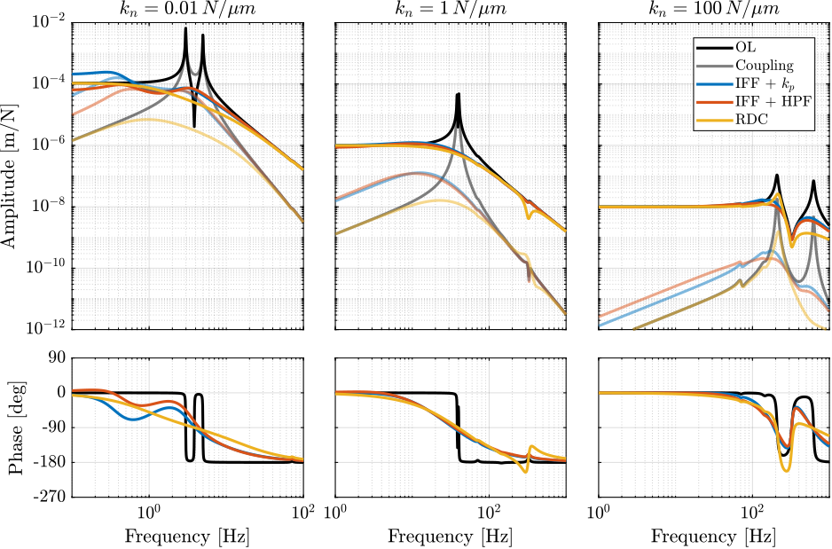
To confirm that the coupling is smaller when the stiffness of the nano-hexapod is increase, the coupling ratio for the three nano-hexapod stiffnesses are shown in Figure ref:fig:rotating_nass_plant_coupling_comp.

Coupling ratio for the proposed active damping techniques evaluated for the three nano-hexapod stiffnesses

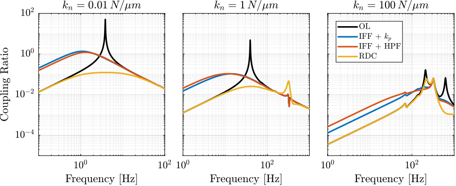
Effect of disturbances

The effect of three disturbances are considered:

• Floor motion (Figure ref:fig:rotating_nass_effect_floor_motion)
• Micro-Station vibrations (Figure ref:fig:rotating_nass_effect_stage_vibration)
• Direct force applied on the payload (Figure ref:fig:rotating_nass_effect_direct_forces)

Conclusions are similar than with the uniaxial (non-rotating) model:

• Regarding the effect of floor motion and forces applied on the payload:

  • The stiffer, the better (magnitudes are lower for the right curves, Figures ref:fig:rotating_nass_effect_floor_motion and ref:fig:rotating_nass_effect_direct_forces)
  • Integral Force Feedback degrades the performances at low frequency compared to relative damping control

• Regarding the effect of micro-station vibrations:

  • Having a soft nano-hexapod allows to filter these vibrations between the suspensions modes of the nano-hexapod and some flexible modes of the micro-station. Using relative damping control reduce this filtering (Figure ref:fig:rotating_nass_effect_stage_vibration, left).

Effect of Floor motion on the position error - Comparison of active damping techniques for the three nano-hexapod stiffnesses

Effect of micro-station vibrations on the position error - Comparison of active damping techniques for the three nano-hexapod stiffnesses

Effect of sample forces on the position error - Comparison of active damping techniques for the three nano-hexapod stiffnesses

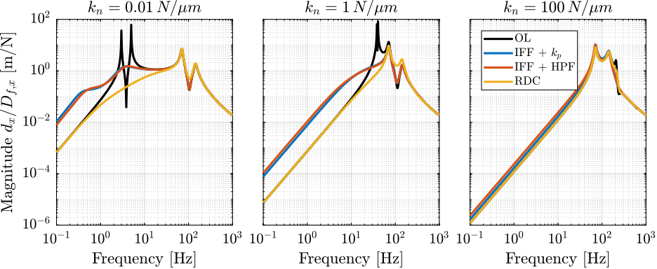
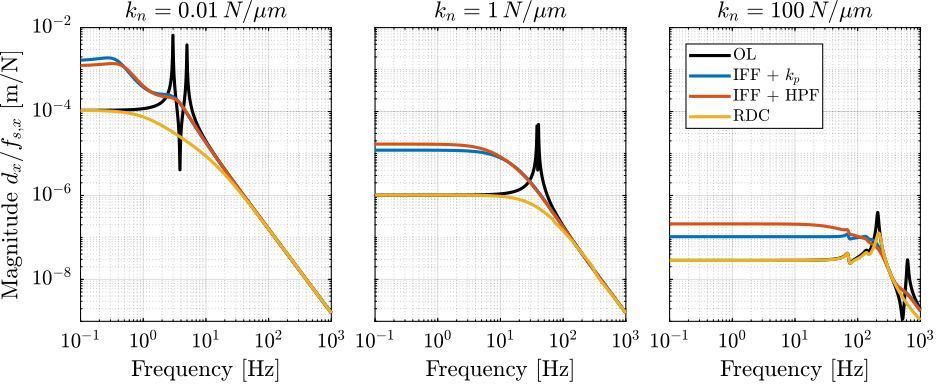
Conclusion

In this study, the gyroscopic effects induced by the spindle's rotation have been studied using a spindle model (Section ref:sec:rotating_system_description). Decentralized IFF with pure integrators was shown to be unstable when applied to rotating platforms (Section ref:sec:rotating_iff_pure_int). Two modifications of the classical IFF control have been proposed to overcome this issue.

The first modification concerns the controller and consists of adding an high pass filter to the pure integrators. This is equivalent as to moving the controller pole to the left along the real axis. This allows the closed loop system to be stable up to some value of the controller gain (Section ref:sec:rotating_iff_pseudo_int).

The second proposed modification concerns the mechanical system. Additional springs are added in parallel with the actuators and force sensors. It was shown that if the stiffness $k_p$ of the additional springs is larger than the negative stiffness $m \Omega^2$ induced by centrifugal forces, the classical decentralized IFF regains its unconditional stability property (Section ref:sec:rotating_iff_parallel_stiffness).

These two modifications were compared with relative damping control in Section ref:sec:rotating_comp_act_damp. While having very different implementations, both proposed modifications were found to be very similar when it comes to the attainable damping and the obtained closed loop system behavior.

Then, this study has been applied to a rotating system that corresponds to the nano-hexapod parameters (Section ref:sec:rotating_nano_hexapod). To be closer to the real system dynamics, the limited compliance of the micro-station has been taken into account. Results show that the two proposed IFF modifications can be applied for the NASS even in the presence of spindle rotation.

Bibliography   ignore