140 KiB
Nano Active Stabilization System - Introduction
- Context of this thesis
- Challenge definition
- Original Contributions
- Introduction
- 6DoF vibration control of a rotating platform
- Mechatronics design approach
- Multi-body simulations with reduced order flexible bodies obtained by FEA
- Control Robustness by design
- Active Damping of rotating mechanical systems using Integral Force Feedback
- Design of complementary filters using $\mathcal{H}_\infty$ Synthesis
- Experimental validation of the Nano Active Stabilization System
- Thesis Outline - Mechatronics Design Approach
- Bibliography
Context of this thesis
Synchrotron Radiation Facilities
Synchrotron radiation facilities, are particle accelerators where electrons are accelerated to near the speed of light. As these electrons traverse magnetic fields, typically generated by insertion devices or bending magnets, they produce exceptionally bright light known as synchrotron light. This intense electromagnetic radiation, particularly in the X-ray spectrum, is subsequently utilized for the detailed study of matter. Approximately 70 synchrotron light sources are operational worldwide, some of which are indicated in Figure ref:fig:introduction_synchrotrons. This global distribution of such facilities underscores the significant utility of synchrotron light for the scientific community.
These facilities fundamentally comprise two main parts: the accelerator complex, where electron acceleration and light generation occur, and the beamlines, where the intense X-ray beams are conditioned and directed for experimental use.
The European Synchrotron Radiation Facility (ESRF), shown in Figure ref:fig:introduction_esrf_picture, is a joint research institution supported by 19 member countries. The ESRF commenced user operations in 1994 as the world's first third-generation synchrotron. Its accelerator complex, schematically depicted in Figure ref:fig:introduction_esrf_schematic, includes a linear accelerator where electrons are initially generated and accelerated, a booster synchrotron to further accelerate the electrons, and an 844-meter circumference storage ring where electrons are maintained in a stable orbit.
Synchrotron light are emitted in more than 40 beamlines surrounding the storage ring, each having specialized experimental stations. These beamlines host diverse instrumentation that enables a wide spectrum of scientific investigations, including structural biology, materials science, and study of matter under extreme conditions.
In August 2020, following an extensive 20-month upgrade period, the ESRF inaugurated its Extremely Brilliant Source (EBS), establishing it as the world's premier fourth-generation synchrotron cite:&raimondi21_commis_hybrid_multib_achrom_lattic. This upgrade implemented a novel storage ring concept that substantially increases the brilliance and coherence of the X-ray beams.
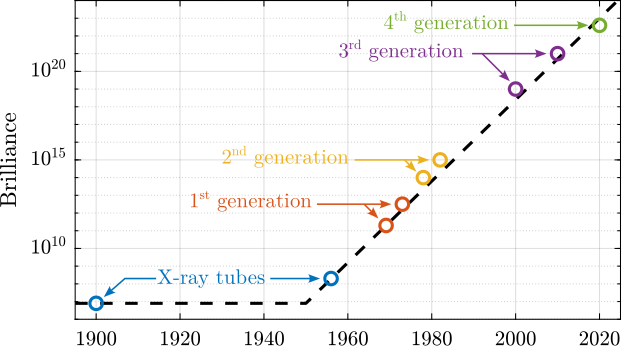
Brilliance, a measure of the photon flux, is a key figure of merit for synchrotron facilities. It experienced an approximate 100-fold increase with the implementation of EBS, as shown in the historical evolution depicted in Figure ref:fig:introduction_moore_law_brillance. While this enhanced beam quality presents unprecedented scientific opportunities, it concurrently introduces considerable engineering challenges, particularly regarding experimental instrumentation and sample positioning systems.
The ID31 ESRF Beamline
Each beamline begins with a "white" beam generated by the insertion device. This beam carries substantial power, typically exceeding kilowatts, and is generally unsuitable for direct application to samples.
Instead, the beam passes through a series of optical elements—including absorbers, mirrors, slits, and monochromators—that filter and shape the X-rays to the desired specifications. These components are housed in multiple Optical Hutches, as depicted in Figure ref:fig:introduction_id31_oh.
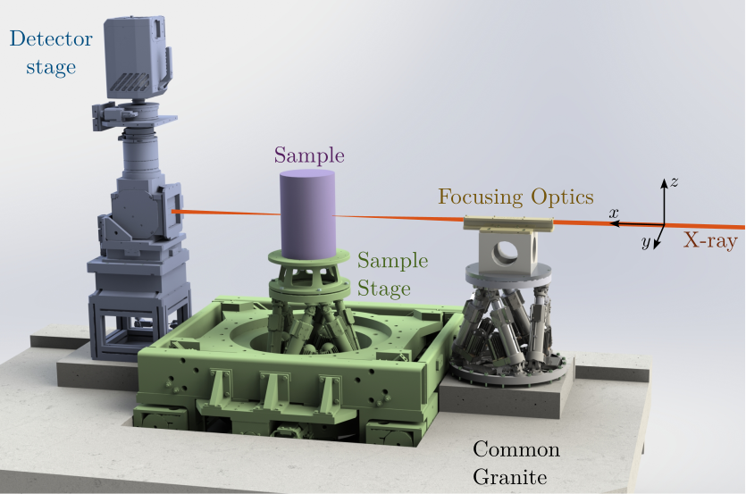
Following the optical hutches, the conditioned beam enters the Experimental Hutch (Figure ref:fig:introduction_id31_cad), where, for experiments pertinent to this work, focusing optics are utilized. The sample is mounted on a positioning stage, referred to as the "end-station", that enables precise alignment relative to the X-ray beam. Detectors are used to capture the X-rays transmitted through or scattered by the sample. Throughout this thesis, the standard ESRF coordinate system is adopted, wherein the X-axis aligns with the beam direction, Y is transverse horizontal, and Z is vertical upwards against gravity.
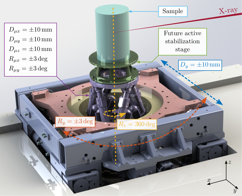
The specific end-station employed on the ID31 beamline is designated the "micro-station". As depicted in Figure ref:fig:introduction_micro_station_dof, it comprises a stack of positioning stages: a translation stage (in blue), a tilt stage (in red), a spindle for continuous rotation (in yellow), and a micro-hexapod (in purple). The sample itself (cyan), potentially housed within complex sample environments (e.g., for high pressure or extreme temperatures), is mounted on top of this assembly. Each stage serves distinct positioning functions; for example, the micro-hexapod enables fine static adjustments, while the $T_y$ translation and $R_z$ rotation stages are utilized for specific scanning applications.
The "stacked-stages" configuration of the micro-station provides high mobility, enabling diverse scientific experiments and imaging techniques. Two illustrative examples are provided.
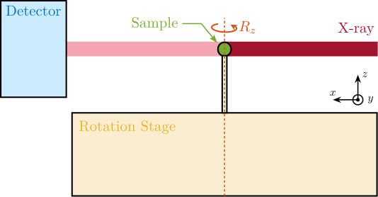
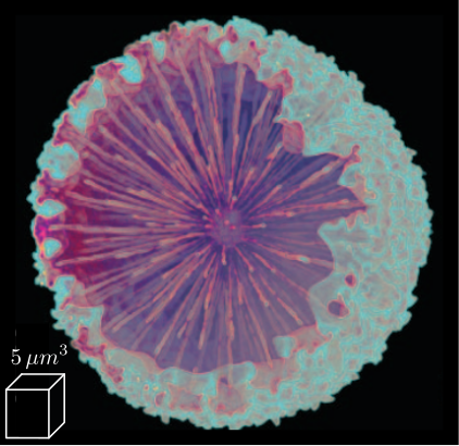
Tomography experiments, schematically represented in Figure ref:fig:introduction_tomography_schematic, involve placing a sample in the X-ray beam path while controlling its vertical rotation angle using a dedicated stage. Detector images are captured at numerous rotation angles, allowing the reconstruction of three-dimensional sample structure (Figure ref:fig:introduction_tomography_results) cite:&schoeppler17_shapin_highl_regul_glass_archit. This reconstruction depends critically on maintaining the sample's point of interest within the beam throughout the rotation process.
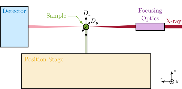
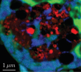
Mapping or scanning experiments, depicted in Figure ref:fig:introduction_scanning_schematic, typically utilize focusing optics to have a small beam size at the sample's location. The sample is then translated perpendicular to the beam (along Y and Z axes), while data is collected at each position. An example cite:&sanchez-cano17_synch_x_ray_fluor_nanop of a resulting two-dimensional map, acquired with 20nm step increments, is shown in Figure ref:fig:introduction_scanning_results. The fidelity and resolution of such images are intrinsically linked to the focused beam size and the positioning precision of the sample relative to the focused beam. Positional instabilities, such as vibrations and thermal drifts, inevitably lead to blurring and distortion in the obtained image. Other advanced imaging modalities practiced on ID31 include reflectivity, diffraction tomography, and small/wide-angle X-ray scattering (SAXS/WAXS).
Need of Accurate Positioning End-Stations with High Dynamics
Continuous advancements in both synchrotron source technology and X-ray optics have led to the availability of smaller, more intense, and more stable X-ray beams. The ESRF-EBS upgrade, for instance, resulted in a significantly reduced source size, particularly in the horizontal dimension, coupled with increased brilliance, as illustrated in Figure ref:fig:introduction_beam_3rd_4th_gen.
Concurrently, substantial progress has been made in micro- and nano-focusing optics since the early days of ESRF, where typical spot sizes were on the order of $10\,\mu m$ cite:&riekel89_microf_works_at_esrf. Various technologies, including zone plates, Kirkpatrick-Baez mirrors, and compound refractive lenses, have been developed and refined, each presenting unique advantages and limitations cite:&barrett16_reflec_optic_hard_x_ray. The historical reduction in achievable spot sizes is represented in Figure ref:fig:introduction_moore_law_focus. Presently, focused beam dimensions in the range of 10 to 20 nm (Full Width at Half Maximum, FWHM) are routinely achieved on specialized nano-focusing beamlines.
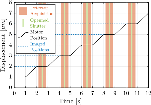
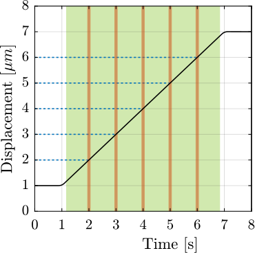
The increased brilliance introduces challenges related to radiation damage, particularly at high-energy beamlines like ID31. Consequently, prolonged exposure of a single sample area to the focused beam must be avoided. Traditionally, experiments were conducted in a "step-scan" mode, illustrated in Figure ref:fig:introduction_scan_step. In this mode, the sample is moved to the desired position, the detector acquisition is initiated, and a beam shutter is opened for a brief, controlled duration to limit radiation damage before closing; this cycle is repeated for each measurement point. While effective for mitigating radiation damage, this sequential process can be time-consuming, especially for high-resolution maps requiring numerous points.
An alternative, more efficient approach is the "fly-scan" or "continuous-scan" methodology cite:&xu23_high_nsls_ii, depicted in Figure ref:fig:introduction_scan_fly. Here, the sample is moved continuously while the detector is triggered to acquire data "on the fly" at predefined positions or time intervals. This technique significantly accelerates data acquisition, enabling better utilization of valuable beamtime while potentially enabling finer spatial resolution cite:&huang15_fly_scan_ptych.
Recent developments in detector technology have yielded sensors with improved spatial resolution, lower noise characteristics, and substantially higher frame rates cite:&hatsui15_x_ray_imagin_detec_synch_xfel_sourc. Historically, detector integration times for scanning and tomography experiments were in the range of 0.1 to 1 second. This extended integration effectively filtered high-frequency vibrations in beam or sample position, resulting in apparently stable but larger beam.
With higher X-ray flux and reduced detector noise, integration times can now be shortened to approximately 1 millisecond, with frame rates exceeding 100 Hz. This reduction in integration time has two major implications for positioning requirements. Firstly, for a given spatial sampling ("pixel size"), faster integration necessitates proportionally higher scanning velocities. Secondly, the shorter integration times make the measurements more susceptible to high-frequency vibrations. Therefore, not only must the sample position be stable against long-term drifts, but it must also be actively controlled to minimize vibrations, especially during dynamic fly-scan acquisitions.
Existing Nano Positioning End-Stations
To contextualize the system developed within this thesis, a brief overview of existing strategies and technologies for high-accuracy, high-dynamics end-stations is provided. The aim is to identify the specific characteristics that distinguish the proposed system from current state-of-the-art implementations.
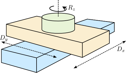
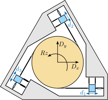
Positioning systems can be broadly categorized based on their kinematic architecture, typically serial or parallel, as exemplified by the 3-Degree-of-Freedom (DoF) platforms in Figure ref:fig:introduction_kinematics. Serial kinematics (Figure ref:fig:introduction_serial_kinematics) utilizes stacked stages where each degree of freedom is controlled by a dedicated actuator. This configuration offers great mobility, but positioning errors (e.g., guiding inaccuracies, thermal expansion) accumulate through the stack, compromising overall accuracy. Similarly, the overall dynamic performance (stiffness, resonant frequencies) is limited by the softest component in the stack, often resulting in poor dynamic behavior when many stages are combined.
Conversely, parallel kinematic architectures (Figure ref:fig:introduction_parallel_kinematics) involve the coordinated motion of multiple actuators to achieve the desired end-effector motion. While theoretically offering the same controlled degrees of freedom as stacked stages, parallel systems generally provide limited stroke but significantly enhanced stiffness and superior dynamic performance.
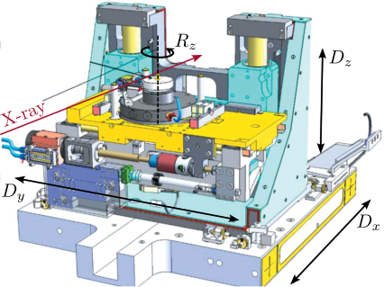
Most end stations, particularly those requiring extensive mobility, employ stacked stages. Their positioning performance consequently depends entirely on the accuracy of individual components. Strategies include employing a limited number of high-performance stages, such as air-bearing spindles cite:&riekel10_progr_micro_nano_diffr_at, and maintaining extremely stable thermal environments within the experimental hutch, often requiring extended stabilization times cite:&leake19_nanod_beaml_id01. Examples of such end-stations, including those at beamlines ID16B cite:&martinez-criado16_id16b and ID11 cite:&wright20_new_oppor_at_mater_scien, are shown in Figure ref:fig:introduction_passive_stations. However, when a large number of DoFs are required, the cumulative errors and limited dynamic stiffness of stacked configurations can make experiments with nano-focused beams extremely challenging or infeasible.
The concept of using an external metrology to measure and potentially correct for positioning errors is increasing used for nano-positioning end-stations. Ideally, the relative position between the sample's point of interest and the X-ray beam focus would be measured directly. In practice, direct measurement is often impossible; instead, the sample position is typically measured relative to a reference frame associated with the focusing optics, providing an indirect measurement.
This measured position can be utilized in several ways: for post-processing correction of acquired data; for calibration routines to compensate for repeatable errors; or, most relevantly here, for real-time feedback control. Various sensor technologies have been employed, with capacitive sensors cite:&schroer17_ptynam;&villar18_nanop_esrf_id16a_nano_imagin_beaml;&schropp20_ptynam and, increasingly, fiber-based interferometers cite:&nazaretski15_pushin_limit;&stankevic17_inter_charac_rotat_stages_x_ray_nanot;&holler17_omny_pin_versat_sampl_holder;&holler18_omny_tomog_nano_cryo_stage;&engblom18_nanop_resul;&schropp20_ptynam;&nazaretski22_new_kirkp_baez_based_scann;&kelly22_delta_robot_long_travel_nano;&xu23_high_nsls_ii;&geraldes23_sapot_carnaub_sirius_lnls being prominent choices.
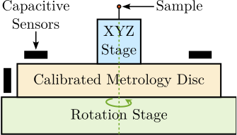
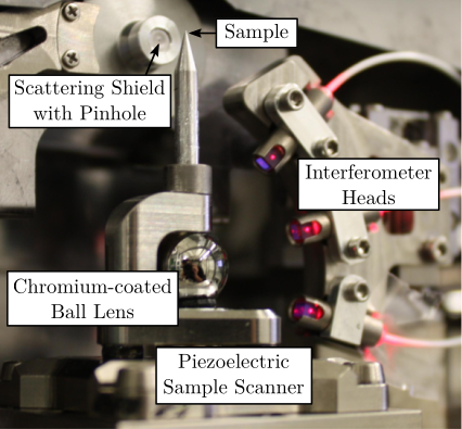
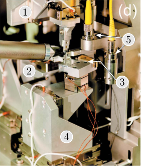
Two examples illustrating the integration of online metrology are presented in Figure ref:fig:introduction_metrology_stations. The system at NSLS X8C (Figure ref:fig:introduction_stages_wang) utilized capacitive sensors for rotation stage calibration and image alignment during tomography post-processing cite:&wang12_autom_marker_full_field_hard. The PtiNAMi microscope at DESY P06 (Figure ref:fig:introduction_stages_schroer) employs interferometers directed at a spherical target below the sample for position monitoring during tomography, with plans for future feedback loop implementation cite:&schropp20_ptynam.
For applications requiring active compensation of measured errors, particularly with nano-beams, feedback control loops are implemented. Actuation is typically achieved using piezoelectric actuators cite:&nazaretski15_pushin_limit;&holler17_omny_pin_versat_sampl_holder;&holler18_omny_tomog_nano_cryo_stage;&villar18_nanop_esrf_id16a_nano_imagin_beaml;&nazaretski22_new_kirkp_baez_based_scann, 3-phase linear motors cite:&stankevic17_inter_charac_rotat_stages_x_ray_nanot;&engblom18_nanop_resul, or voice coil actuators cite:&kelly22_delta_robot_long_travel_nano;&geraldes23_sapot_carnaub_sirius_lnls. While often omitted, feedback bandwidth for such stages are relatively low (around 1 Hz), primarily targeting the compensation of slow thermal drifts. More recently, higher bandwidths (up to 100 Hz) have been demonstrated, particularly with the use of voice coil actuators cite:&kelly22_delta_robot_long_travel_nano;&geraldes23_sapot_carnaub_sirius_lnls.
Figure ref:fig:introduction_active_stations showcases two end-stations incorporating online metrology and active feedback control. The ID16A system at ESRF (Figure ref:fig:introduction_stages_villar) uses capacitive sensors and a piezoelectric hexapod to compensate for rotation stage errors and to perform accurate scans cite:&villar18_nanop_esrf_id16a_nano_imagin_beaml. Another example, shown in Figure ref:fig:introduction_stages_nazaretski, employs interferometers and piezoelectric stages to compensate for thermal drifts cite:&nazaretski15_pushin_limit;&nazaretski17_desig_perfor_x_ray_scann. A more comprehensive review of actively controlled end-stations is provided in Section ref:sec:nhexa_platform_review.
For tomography experiments, correcting spindle guiding errors is critical. Correction stages are typically placed either below the spindle cite:&stankevic17_inter_charac_rotat_stages_x_ray_nanot;&holler17_omny_pin_versat_sampl_holder;&holler18_omny_tomog_nano_cryo_stage;&villar18_nanop_esrf_id16a_nano_imagin_beaml;&engblom18_nanop_resul;&nazaretski22_new_kirkp_baez_based_scann;&xu23_high_nsls_ii or above it cite:&wang12_autom_marker_full_field_hard;&schroer17_ptynam;&schropp20_ptynam;&geraldes23_sapot_carnaub_sirius_lnls. In most reported cases, only translation errors are actively corrected. Payload capacities for these high-precision systems are usually limited, typically handling calibrated samples on the micron scale, although capacities up to 500g have been reported cite:&nazaretski22_new_kirkp_baez_based_scann;&kelly22_delta_robot_long_travel_nano. The system developed in this thesis aims for payload capabilities approximately 100 times heavier (up to 50 kg) than previous stations with similar positioning requirements.
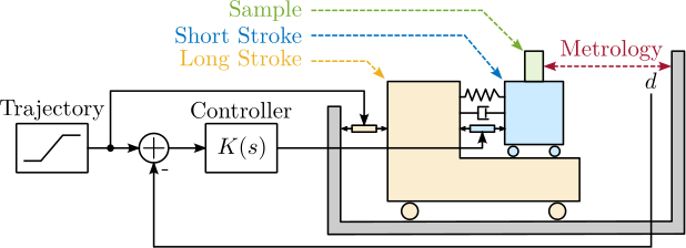
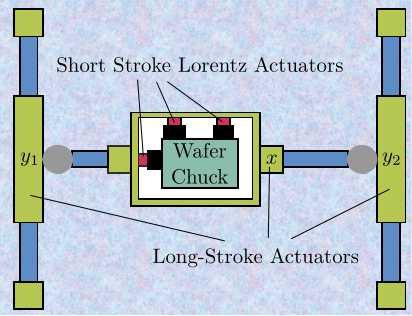
End-stations integrating online metrology for active nano-positioning often exhibit limited operational ranges, typically constrained to a few degrees of freedom with strokes around $100\,\mu m$. Recently, voice coil actuators were used to increase the stroke up to $3\,\text{mm}$ cite:&kelly22_delta_robot_long_travel_nano;&geraldes23_sapot_carnaub_sirius_lnls An alternative strategy involves a "long stroke-short stroke" architecture, illustrated conceptually in Figure ref:fig:introduction_two_stage_schematic. In this configuration, a high-accuracy, high-bandwidth short-stroke stage is mounted on top of a less precise long-stroke stage. The short-stroke stage actively compensates for errors based on metrology feedback, while the long-stroke stage performs the larger movements. This approach allows combining extended travel with high precision and good dynamical response, but is often implemented for only one or a few DoFs, as seen in Figures ref:fig:introduction_two_stage_schematic and ref:fig:introduction_two_stage_control_h_bridge.
Challenge definition
Introduction ignore
The advent of fourth-generation light sources, coupled with advancements in focusing optics and detector technology, imposes stringent new requirements on sample positioning systems.
With ID31's anticipated minimum beam dimensions of approximately $200\,\text{nm}\times 100\,\text{nm}$, the primary experimental objective is maintaining the sample's point of interest within this beam. This necessitates peak-to-peak positioning errors below $200\,\text{nm}$ in $D_y$ and $200\,\text{nm}$ in $D_z$, corresponding to RMS errors of $30\,\text{nm}$ and $15\,\text{nm}$, respectively. Additionally, the $R_y$ tilt angle error must remain below $0.1\,\text{mdeg}$ ($250\,\text{nrad RMS}$). Given the high frame rates of modern detectors, these specified positioning errors must be maintained even when considering high-frequency vibrations.
These demanding stability requirements must be achieved within the specific context of the ID31 beamline, which necessitates the integration with the existing micro-station, accommodating a wide range of experimental configurations requiring high mobility, and handling substantial payloads up to 50 kg.
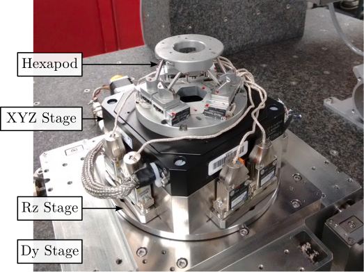
The existing micro-station, despite being composed of high-performance stages, exhibits positioning accuracy limited to approximately $10\,\mu m$ and $10\,\mu\text{rad}$ due to inherent factors such as backlash, mechanical play, thermal expansion, imperfect guiding, and vibrations.
The primary objective of this project is therefore defined as enhancing the positioning accuracy and stability of the ID31 micro-station by roughly two orders of magnitude, to fully leverage the capabilities offered by the ESRF-EBS source and modern detectors, without compromising its existing mobility and payload capacity.
The Nano Active Stabilization System Concept
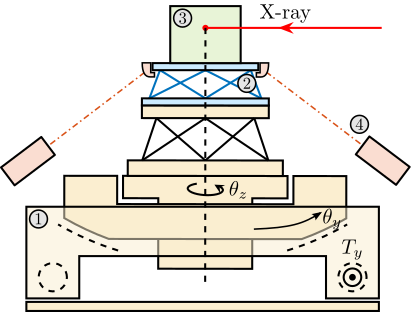
To address these challenges, the concept of a Nano Active Stabilization System (NASS) is proposed. As schematically illustrated in Figure ref:fig:introduction_nass_concept_schematic, the NASS comprises four principal components integrated with the existing micro-station (yellow): a 5-DoF online metrology system (red), an active stabilization platform (blue), and the associated control system and instrumentation (purple). This system essentially functions as a high-performance, multi-axis vibration isolation and error correction platform situated between the micro-station and the sample. It actively compensates for positioning errors measured by the external metrology system.
Online Metrology system
The performance of the NASS is fundamentally reliant on the accuracy and bandwidth of its online metrology system, as the active control is based directly on these measurements. This metrology system must fulfill several criteria: measure the sample position in 5 DoF (excluding rotation about the vertical Z-axis); possess a measurement range compatible with the micro-station's extensive mobility and continuous spindle rotation; achieve an accuracy compatible with the sub-100 nm positioning target; and offer high bandwidth for real-time control.
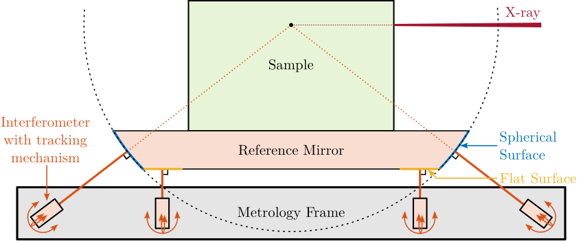
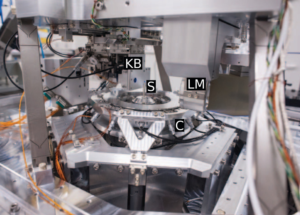
A proposed concept (illustrated in Figure ref:fig:introduction_nass_metrology) features a spherical reflector with a flat bottom attached below the sample, with its center aligned to the X-ray focus. Fiber interferometers target both surfaces. A tracking system maintains perpendicularity between the interferometer beams and the mirror, such that Abbe errors are eliminated. Interferometers pointing at the spherical surface provides translation measurement, while the ones pointing at the flat bottom surface yield tilt angles. The development of this complex metrology system constitutes a significant mechatronic project in itself and is currently ongoing; it is not further detailed within this thesis. For the work presented herein, the metrology system is assumed to provide accurate, high-bandwidth 5-DoF position measurements.
Active Stabilization Platform Design
The active stabilization platform, positioned between the micro-station top plate and the sample, must satisfy several demanding requirements. It needs to provide active motion compensation in 5 degrees of freedom ($D_x$, $D_y$, $D_z$, $R_x$ and $R_y$). It must possess excellent dynamic properties to enable high-bandwidth control capable of suppressing vibrations and tracking desired trajectories with nanometer-level precision. Consequently, it must be free from backlash and play, and its active components (e.g., actuators) should introduce minimal vibrations. Critically, it must accommodate payloads up to 50 kg.
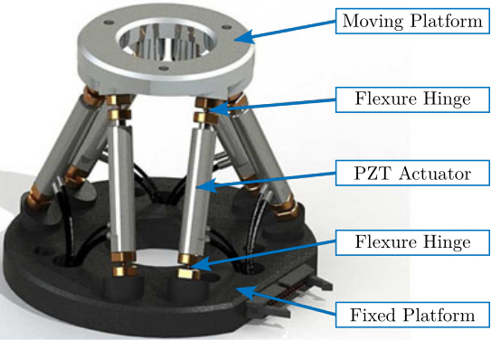
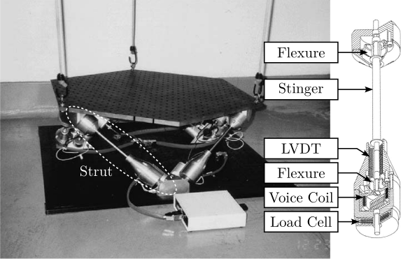
A suitable candidate architecture for this platform is the Stewart platform (also known as "hexapod"), a parallel kinematic mechanism capable of 6-DoF motion. Stewart platforms are widely employed in positioning and vibration isolation applications due to their inherent stiffness and potential for high precision. Various designs exist, differing in geometry, actuation technology, sensing methods, and control strategies, as exemplified in Figure ref:fig:introduction_stewart_platform_piezo. A central challenge addressed in this thesis is the optimal mechatronic design of such an active platform tailored to the specific requirements of the NASS. A more detailed review of Stewart platform and its main components will be given in Section ref:sec:detail_kinematics_stewart_review.
Robust Control
The control system must compute the position measurements from the online metrology system and computes the reference positions derived from each micro-station desired movement. It then commands the active platform in real time to stabilize the sample and compensate for all error sources, including stage imperfections, thermal drifts, and vibrations. Ensuring the stability and robustness of these feedback loops is crucial, especially within the demanding operational context of a synchrotron beamline, which requires reliable 24/7 operation with minimal intervention.
Several factors complicate the design of robust feedback control for the NASS. First, the system must operate under across diverse experimental conditions, including different scan types (tomography, linear scans) and payloads' inertia. The continuous rotation of the spindle introduces gyroscopic effects that can affect the system dynamics. As actuators of the active platforms rotate relative to stationary sensors, the control kinematics to map the errors in the frame of the active platform is complex. But perhaps the most significant challenge is the wide variation in payload mass (1 kg up to 50 kg) that the system must accommodate. Designing for robustness against large payload variations typically necessitates larger stability margins, which can compromise achievable performance. Consequently, high-performance positioning stages often work with well-characterized payload, as seen in systems like wafer-scanners or atomic force microscopes.
Furthermore, unlike many systems where the active stage and sample are significantly lighter than the underlying coarse stages, the NASS payload mass can be substantially greater than the mass of the micro-station's top stage. This leads to strong dynamic coupling between the active platform and the micro-station structure, resulting in a more complex multi-inputs multi-outputs (MIMO) system with significant cross-talk between axes.
These variations in operating conditions and payload translate into significant uncertainty or changes in the plant dynamics that the controller must handle. Therefore, the feedback controller must be designed to be robust against this plant uncertainty while still delivering the required nanometer-level performance.
Predictive Design / Mechatronics approach
The overall performance achieved by the NASS is determined by numerous factors, such as external disturbances, the noise characteristics of the instrumentation, the dynamics resulting from the chosen mechanical architecture, and the achievable bandwidth dictated by the control architecture. Ensuring the final system met its stringent specifications requires the implementation of a predictive design methodology, also known as a mechatronics design approach. The goal is to rigorously evaluate different concepts, predict performance limitations, and guide the design process. Key challenges within this approach include developing appropriate design methodologies, creating accurate models capable of comparing different concepts quantitatively, and converging on a final design that achieves the target performance levels.
Original Contributions
Introduction ignore
This thesis presents several original contributions aimed at addressing the challenges inherent in the design, control, and implementation of the Nano Active Stabilization System, primarily within the fields of Control Theory, Mechatronics Design, and Experimental Validation.
6DoF vibration control of a rotating platform
Traditional long-stroke/short-stroke architectures typically operate in one or two degrees of freedom. This work extends the concept to six degrees of freedom, with the active platform designed not only to correct rotational errors but to simultaneously compensate for errors originating from all underlying micro-station stages. The application of a continuously rotating Stewart platform for active vibration control and error compensation in this manner is believed to be novel in the reviewed literature.
Mechatronics design approach
A rigorous mechatronics design methodology was applied consistently throughout the NASS development lifecycle cite:&dehaeze18_sampl_stabil_for_tomog_exper;&dehaeze21_mechat_approac_devel_nano_activ_stabil_system. Although the mechatronics approach itself is not new, its comprehensive application here, from initial concept evaluation using simplified models to detailed design optimization and experimental validation informed by increasingly sophisticated models, potentially offers useful insights to the existing literature. This thesis documents this process chronologically, illustrating how models of varying complexity can be effectively utilized at different project phases and how design decisions were systematically based on quantitative model predictions and analyses. While the resulting system is highly specific, the documented effectiveness of this design approach may contribute to the broader adoption of mechatronics methodologies in the design of future synchrotron instrumentation.
Multi-body simulations with reduced order flexible bodies obtained by FEA
A key tool employed extensively in this work was a combined multi-body simulation and Finite Element Analysis technique, specifically utilizing Component Mode Synthesis to represent flexible bodies within the multi-body framework cite:&brumund21_multib_simul_reduc_order_flexib_bodies_fea. This hybrid approach, while established, was experimentally validated in this work for components critical to the NASS, namely amplified piezoelectric actuators and flexible joints. It proved invaluable for designing and optimizing components intended for integration into a larger, complex dynamic system. This methodology, detailed in Section ref:sec:detail_fem, is presented as a potentially useful tool for future mechatronic instrument development.
Control Robustness by design
The requirement for robust operation across diverse conditions—including payloads up to 50kg, complex underlying dynamics from the micro-station, and varied operational modes like different rotation speeds—presented a critical design challenge. This challenge was met by embedding robustness directly into the active platform's design, rather than depending solely on complex post-design control synthesis techniques such as $\mathcal{H}_\infty\text{-synthesis}$ and $\mu\text{-synthesis}$. Key elements of this strategy included the model-based evaluation of active stage designs to identify architectures inherently easier to control, the incorporation of collocated actuator/sensor pairs to leverage passivity-based guaranteed stability, and the comparison of architecture to combine several sensors such as sensor fusion and High Authority Control / Low Authority Control (HAC-LAC). Furthermore, decoupling strategies for parallel manipulators were compared (Section ref:sec:detail_control_decoupling), addressing a topic identified as having limited treatment in the literature. Consequently, the specified performance targets were met utilizing controllers which, facilitated by this design approach, proved to be robust, readily tunable, and easily maintained.
Active Damping of rotating mechanical systems using Integral Force Feedback
During conceptual design, it was found that the guaranteed stability property of the established active damping technique known as Integral Force Feedback (IFF) is compromised when applied to rotating platforms like the NASS. To address this instability issue, two modifications to the classical IFF control scheme were proposed and analyzed. The first involves a minor adjustment to the control law itself, while the second incorporates physical springs in parallel with the force sensors. Stability conditions and optimal parameter tuning guidelines were derived for both modified schemes. This is further discussed in Section ref:sec:rotating and was the subject of publications cite:&dehaeze20_activ_dampin_rotat_platf_integ_force_feedb;&dehaeze21_activ_dampin_rotat_platf_using.
Design of complementary filters using $\mathcal{H}_\infty$ Synthesis
For implementing sensor fusion, where signals from multiple sensors are combined, complementary filters are often employed. A novel method for designing these filters using $\mathcal{H}_\infty$ synthesis techniques was developed cite:&dehaeze19_compl_filter_shapin_using_synth. This method allows explicit shaping of the filter norms, providing guarantees on the performance of the sensor fusion process. This synthesis technique, discussed further in Section ref:sec:detail_control_sensor, has subsequently found application in optimizing sensor fusion for gravitational wave detectors cite:&tsang22_optim_sensor_fusion_method_activ. The integration of such filters into feedback control architectures can also lead to advantageous control structures, as proposed in cite:&verma20_virtual_sensor_fusion_high_precis_contr and further studied in Section ref:sec:detail_control_cf.
Experimental validation of the Nano Active Stabilization System
The conclusion of this work involved the experimental implementation and validation of the complete NASS on the ID31 beamline. Experimental results, presented in Section ref:sec:test_id31, demonstrate that the system successfully improves the effective positioning accuracy of the micro-station from its native $\approx 10\,\mu m$ level down to the target $\approx 100\,nm$ range during representative scientific experiments. Crucially, robustness to variations in sample mass and diverse experimental conditions was verified. The NASS thus provides a versatile end-station solution, uniquely combining high payload capacity with nanometer-level accuracy, enabling optimal utilization of the advanced capabilities of the ESRF-EBS beam and associated detectors. To the author's knowledge, this represents the first demonstration of such a 5-DoF active stabilization platform being used to enhance the accuracy of a complex positioning system to this level.
Thesis Outline - Mechatronics Design Approach
Introduction ignore
This thesis is structured chronologically, mirroring the phases of the mechatronics development approach employed for the NASS project. It is divided into three chapters, each corresponding to a distinct phase of this methodology: Conceptual Design, Detailed Design, and Experimental Validation. While the chapters follow this logical progression, care has been taken to structure each chapter such that its constitutive sections may also be consulted independently based on the reader's specific interests.
Conceptual design development
The conceptual design phase, detailed in Chapter ref:chap:concept, followed a methodical progression from simplified uniaxial models to more complex multi-body representations. Initial uniaxial analysis (Section ref:sec:uniaxial) provided fundamental insights, particularly regarding the influence of active platform stiffness on performance. The introduction of rotation in a 3-DoF model (Section ref:sec:rotating) allowed investigation of gyroscopic effects, revealing challenges for softer platform designs. Experimental modal analysis of the existing micro-station (Section ref:sec:modal) confirmed its complex dynamics but supported a rigid-body assumption for the different stages, justifying the development of a detailed multi-body model. This model, tuned against experimental data and incorporating measured disturbances, was validated through simulation (Section ref:sec:ustation). The Stewart platform architecture was selected for the active stage, and its kinematics, dynamics, and control were analyzed (Section ref:sec:nhexa). The chapter culminates in Section ref:sec:nass with closed-loop simulations of the integrated NASS concept under realistic conditions, validating its feasibility and providing confidence for proceeding to the detailed design phase. Dynamic error budgeting cite:&monkhorst04_dynam_error_budget;&okyay16_mechat_desig_dynam_contr_metrol was employed throughout this phase to identify performance limitations and guide concept selection.
Detailed design
Chapter ref:chap:detail focuses on translating the validated NASS concept into an optimized, implementable design. Building upon the conceptual model which used idealized components, this phase addresses the detailed specification and optimization of each subsystem. It starts with the determination of the optimal nano-hexapod geometry (Section ref:sec:detail_kinematics), analyzing the influence of geometric parameters on mobility, stiffness, and dynamics, leading to specific requirements for actuator stroke and joint mobility. A hybrid multi-body/FEA modeling methodology is introduced and experimentally validated (Section ref:sec:detail_fem), then applied to optimize the actuators (Section ref:sec:detail_fem_actuator) and flexible joints (Section ref:sec:detail_fem_joint) while maintaining system-level simulation capability. Control strategy refinement (Section ref:sec:detail_control) involves optimal integration of multiple sensors in the control architecture, evaluating decoupling strategies, and discussing controller optimization for decoupled systems. Instrumentation selection (Section ref:sec:detail_instrumentation) is guided by dynamic error budgeting to establish noise specifications, followed by experimental characterization. The chapter concludes (Section ref:sec:detail_design) by presenting the final, optimized nano-hexapod design, ready for procurement and assembly.
Experimental validation
Chapter ref:chap:test details the experimental validation process, proceeding systematically from component-level characterization to full system evaluation on the beamline. Actuators of the active platform were characterized, models validated, and active damping (IFF) tested (Section ref:sec:test_apa). Flexible joints were tested on a dedicated bench to verify stiffness and stroke specifications (Section ref:sec:test_joints). Assembled struts (actuators + joints) were then characterized to ensure consistency and validate multi-body models (Section ref:sec:test_struts). The complete nano-hexapod assembly was tested on an isolated table, allowing accurate dynamic identification and model validation under various payload conditions (Section ref:sec:test_nhexa). Finally, the integrated NASS was validated on the ID31 beamline using a purpose-built short-stroke metrology system (Section ref:sec:test_id31). The implemented control architecture was tested under realistic experimental scenarios, including tomography with heavy payloads, confirming the system's performance and robustness.
