phd-nass-geometry/nass-geometry.org

Nano Hexapod - Optimal Geometry

• Introduction
• Review of Stewart platforms
  • Introduction
• Effect of geometry on Stewart platform properties
  • Introduction
  • Platform Mobility
    • Introduction
    • Mobility in translation
    • Mobility in rotation
    • Combined translations and rotations
  • Stiffness
    • Introduction
    • Translation Stiffness
    • Rotational Stiffness
    • Diagonal Stiffness Matrix
  • Dynamical properties
    • In the Cartesian Frame
    • In the frame of the Struts
    • Dynamic Isotropy
  • Conclusion
• The Cubic Architecture
  • Introduction
  • The Cubic Architecture
  • Static Properties
    • Uniform stiffness
    • Uniform Mobility
  • Dynamical Decoupling
    • Introduction
    • Cube's center at the Center of Mass of the mobile platform
    • Cube's center not coincident with the Mass of the Mobile platform
    • Dynamic isotropy
    • Conclusion
  • Decentralized Control
    • Introduction
    • Cubic Architecture
    • Non-Cubic Architecture
    • Conclusion
  • Cubic architecture with Cube's center above the top platform
    • Introduction
    • Small cube
    • Medium sized cube
    • Large cube
    • Required size of the platforms
    • Conclusion
  • Conclusion
• Conclusion
• Bibliography

Introduction   ignore

• In the conceptual design phase, the geometry of the Stewart platform was chosen arbitrarily and not optimized
• In the detail design phase, we want to see if the geometry can be optimized to improve the overall performances
• Optimization criteria: mobility, stiffness, dynamical decoupling, more performance / bandwidth

Outline:

• Review of Stewart platform (Section ref:sec:detail_kinematics_stewart_review) Geometry, Actuators, Sensors, Joints
• Effect of geometry on the Stewart platform characteristics (Section ref:sec:detail_kinematics_geometry)
• Cubic configuration: benefits? (Section ref:sec:detail_kinematics_cubic)
• Obtained geometry for the nano hexapod (Section ref:sec:detail_kinematics_nano_hexapod)

Review of Stewart platforms

<<sec:detail_kinematics_stewart_review>>

Introduction   ignore

• As was explained in the conceptual phase, Stewart platform have the following key elements:

  • Two plates connected by six struts

  • Each strut is composed of:

    • a flexible joint at each end
    • an actuator
    • one or several sensors
• The exact geometry (i.e. position of joints and orientation of the struts) can be chosen freely depending on the application.
• This results in many different designs found in the literature.
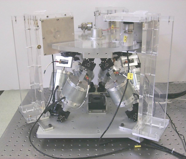
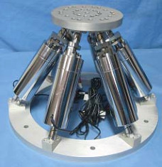
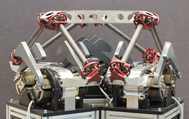
• The focus is here made on Stewart platforms for nano-positioning and vibration control. Long stroke stewart platforms are not considered here as their design impose other challenges. Some Stewart platforms found in the literature are listed in Table ref:tab:detail_kinematics_stewart_review
• All presented Stewart platforms are using flexible joints, as it is a prerequisites for nano-positioning capabilities.

• Most of stewart platforms are using voice coil actuators or piezoelectric actuators. The actuators used for the Stewart platform will be chosen in the next section.

• Depending on the application, various sensors are integrated in the struts or on the plates. The choice of sensor for the nano-hexapod will be described in the next section.

• There are two categories of Stewart platform geometry:

  • Cubic architecture (Figure ref:fig:detail_kinematics_stewart_examples_cubic). Struts are positioned along 6 sides of a cubic (and are therefore orthogonal to each other). Such specific architecture has some special properties that will be studied in Section ref:sec:detail_kinematics_cubic.
  • Non-cubic architecture (Figure ref:fig:detail_kinematics_stewart_examples_non_cubic)

\bigskip

\bigskip

	Geometry	Actuators	Sensors	Reference
	Cubic	Magnetostrictive	Force, Accelerometers	cite:&geng93_six_degree_of_freed_activ;&geng94_six_degree_of_freed_activ;&geng95_intel_contr_system_multip_degree
Figure ref:fig:detail_kinematics_jpl	Cubic	Voice Coil (0.5 mm)	Force	cite:&spanos95_soft_activ_vibrat_isolat;&rahman98_multiax
	Cubic	Voice Coil (10 mm)	Force, LVDT, Geophones	cite:&thayer98_stewar;&thayer02_six_axis_vibrat_isolat_system;&hauge04_sensor_contr_space_based_six
Figure ref:fig:detail_kinematics_uw_gsp	Cubic	Voice Coil	Force	cite:&mcinroy99_dynam;&mcinroy99_precis_fault_toler_point_using_stewar_platf;&mcinroy00_desig_contr_flexur_joint_hexap;&li01_simul_vibrat_isolat_point_contr;&jafari03_orthog_gough_stewar_platf_microm
	Cubic	Piezoelectric ($25\,\mu m$)	Force	cite:&defendini00_techn
Figure ref:fig:detail_kinematics_ulb_pz	Cubic	APA ($50\,\mu m$)	Force	cite:&abu02_stiff_soft_stewar_platf_activ
Figure ref:fig:detail_kinematics_pph	Non-Cubic	Voice Coil	Accelerometers	cite:&chen03_payload_point_activ_vibrat_isolat
	Cubic	Voice Coil	Force	cite:&hanieh03_activ_stewar;&preumont07_six_axis_singl_stage_activ
Figure ref:fig:detail_kinematics_uqp	Cubic	Piezoelectric ($50\,\mu m$)	Geophone	cite:&agrawal04_algor_activ_vibrat_isolat_spacec
	Non-Cubic	Piezoelectric ($16\,\mu m$)	Eddy Current	cite:&furutani04_nanom_cuttin_machin_using_stewar
	Cubic	Piezoelectric ($120\,\mu m$)	(External) Capacitive	cite:&ting06_desig_stewar_nanos_platf;&ting13_compos_contr_desig_stewar_nanos_platf
	Non-Cubic	Piezoelectric ($160\,\mu m$)	(External) Capacitive	cite:&ting07_measur_calib_stewar_microm_system
Figure ref:fig:detail_kinematics_zhang11	Non-cubic	Magnetostrictive	Accelerometer	cite:&zhang11_six_dof
	Non-Cubic	Piezoelectric	Strain Gauge	cite:&du14_piezo_actuat_high_precis_flexib
	Cubic	Voice Coil	Accelerometer	cite:&chi15_desig_exper_study_vcm_based;&tang18_decen_vibrat_contr_voice_coil;&jiao18_dynam_model_exper_analy_stewar
	Cubic	Piezoelectric	Force	cite:&wang16_inves_activ_vibrat_isolat_stewar
	Almost cubic	Voice Coil	Force, Accelerometer	cite:&beijen18_self_tunin_mimo_distur_feedf;&tjepkema12_activ_ph
Figure ref:fig:detail_kinematics_yang19	Almost cubic	Piezoelectric	Force, Strain gauge	cite:&yang19_dynam_model_decoup_contr_flexib
Figure ref:fig:detail_kinematics_naves	Non-Cubic	3-phase rotary motor	Rotary Encoder	cite:&naves20_desig;&naves20_t_flex

Conclusion:

• Various Stewart platform designs:

  • geometry, sizes, orientation of struts
  • Lot's have a "cubic" architecture that will be discussed in Section ref:sec:detail_kinematics_cubic
  • actuator types
  • various sensors
  • flexible joints (discussed in next chapter)
• The effect of geometry on the properties of the Stewart platform is studied in section ref:sec:detail_kinematics_geometry
• It is determined what is the optimal geometry for the NASS

Effect of geometry on Stewart platform properties

<<sec:detail_kinematics_geometry>>

Introduction   ignore

• As was shown during the conceptual phase, the geometry of the Stewart platform influences:

  • the stiffness and compliance properties
  • the mobility
  • the force authority
  • the dynamics of the manipulator
• It is therefore important to understand how the geometry impact these properties, and to be able to optimize the geometry for a specific application.

One important tool to study this is the Jacobian matrix which depends on the $\bm{b}_i$ (join position w.r.t top platform) and $\hat{\bm{s}}_i$ (orientation of struts). The choice of frames ($\{A\}$ and $\{B\}$), independently of the physical Stewart platform geometry, impacts the obtained kinematics and stiffness matrix, as it is defined for forces and motion evaluated at the chosen frame.

Platform Mobility

Introduction   ignore

The mobility of the Stewart platform (or any manipulator) is here defined as the range of motion that it can perform. It corresponds to the set of possible pose (i.e. combined translation and rotation) of frame {B} with respect to frame {A}. It should therefore be represented in a six dimensional space.

As was shown during the conceptual phase, for small displacements, the Jacobian matrix can be used to link the strut motion to the motion of frame B with respect to A through equation eqref:eq:detail_kinematics_jacobian.

\begin{equation}\label{eq:detail_kinematics_jacobian} \begin{bmatrix} \delta l_1 \\ \delta l_2 \\ \delta l_3 \\ \delta l_4 \\ \delta l_5 \\ \delta l_6 \end{bmatrix} = \begin{bmatrix} {{}^A\hat{\bm{s}}_1}^T & ({}^A\bm{b}_1 \times {}^A\hat{\bm{s}}_1)^T \\ {{}^A\hat{\bm{s}}_2}^T & ({}^A\bm{b}_2 \times {}^A\hat{\bm{s}}_2)^T \\ {{}^A\hat{\bm{s}}_3}^T & ({}^A\bm{b}_3 \times {}^A\hat{\bm{s}}_3)^T \\ {{}^A\hat{\bm{s}}_4}^T & ({}^A\bm{b}_4 \times {}^A\hat{\bm{s}}_4)^T \\ {{}^A\hat{\bm{s}}_5}^T & ({}^A\bm{b}_5 \times {}^A\hat{\bm{s}}_5)^T \\ {{}^A\hat{\bm{s}}_6}^T & ({}^A\bm{b}_6 \times {}^A\hat{\bm{s}}_6)^T \end{bmatrix} \begin{bmatrix} \delta x \\ \delta y \\ \delta z \\ \delta \theta_x \\ \delta \theta_y \\ \delta \theta_z \end{bmatrix} = \begin{bmatrix} {{}^A\hat{\bm{s}}_1}^T & ({}^A\bm{b}_1 \times {}^A\hat{\bm{s}}_1)^T \\ {{}^A\hat{\bm{s}}_2}^T & ({}^A\bm{b}_2 \times {}^A\hat{\bm{s}}_2)^T \\ {{}^A\hat{\bm{s}}_3}^T & ({}^A\bm{b}_3 \times {}^A\hat{\bm{s}}_3)^T \\ {{}^A\hat{\bm{s}}_4}^T & ({}^A\bm{b}_4 \times {}^A\hat{\bm{s}}_4)^T \\ {{}^A\hat{\bm{s}}_5}^T & ({}^A\bm{b}_5 \times {}^A\hat{\bm{s}}_5)^T \\ {{}^A\hat{\bm{s}}_6}^T & ({}^A\bm{b}_6 \times {}^A\hat{\bm{s}}_6)^T \end{bmatrix} \begin{bmatrix} \delta x \\ \delta y \\ \delta z \\ \delta \theta_x \\ \delta \theta_y \\ \delta \theta_z \end{bmatrix} \begin{bmatrix} \delta x \\ \delta y \\ \delta z \\ \delta \theta_x \\ \delta \theta_y \\ \delta \theta_z \end{bmatrix}

\end{equation}

Therefore, the mobility of the Stewart platform (set of $[\delta x\ \delta y\ \delta z\ \delta \theta_x\ \delta \theta_y\ \delta \theta_z]$) depends on:

• the stroke of each strut
• the geometry of the Stewart platform (embodied in the Jacobian matrix)

More specifically:

• the XYZ mobility only depends on the si (orientation of struts)
• the mobility in rotation depends on bi (position of top joints)

As will be shown in Section ref:sec:detail_kinematics_cubic, there are some geometry that gives same stroke in X, Y and Z directions.

As the mobility is of dimension six, it is difficult to represent. Depending on the applications, only the translation mobility or the rotation mobility may be represented.

Mobility in translation

Here, for simplicity, only translations are first considered:

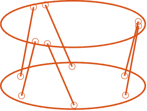
• Let's consider a general Stewart platform geometry shown in Figure ref:fig:detail_kinematics_mobility_trans_arch.
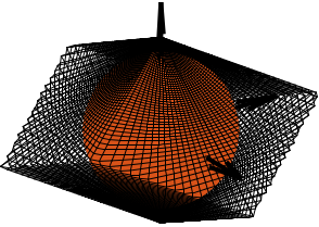
• In the general case: the translational mobility can be represented by a 3D shape with 12 faces (each actuator limits the stroke along its orientation in positive and negative directions). The faces are therefore perpendicular to the strut direction. The obtained mobility is shown in Figure ref:fig:detail_kinematics_mobility_trans_result.
• Considering an actuator stroke of $\pm d$, the mobile platform can be translated in any direction with a stroke of $d$ A circle with radius $d$ can be contained in the general shape. It will touch the shape along six lines defined by the strut axes. The sphere with radius $d$ is shown in Figure ref:fig:detail_kinematics_mobility_trans_result.
• Therefore, for any (small stroke) Stewart platform with actuator stroke $\pm d$, it is possible to move the top platform in any direction by at least a distance $d$. Note that no platform angular motion is here considered. When combining angular motion, the linear stroke decreases.
• When considering some symmetry in the system (as typically the case), the shape becomes a Trigonal trapezohedron whose height and width depends on the orientation of the struts. We only get 6 faces as usually the Stewart platform consists of 3 sets of 2 parallels struts.

thetas = linspace(0, pi, 100);
phis = linspace(0, 2*pi, 100);
rs = zeros(length(thetas), length(phis));

for i = 1:length(thetas)
    for j = 1:length(phis)
        Tx = sin(thetas(i))*cos(phis(j));
        Ty = sin(thetas(i))*sin(phis(j));
        Tz = cos(thetas(i));

        dL = stewart.kinematics.J*[Tx; Ty; Tz; 0; 0; 0;]; % dL required for 1m displacement in theta/phi direction

        rs(i, j) = L_max/max(abs(dL));
    end
end

% Sphere with radius equal to actuator stroke
[Xs,Ys,Zs] = sphere;
Xs = 1e6*L_max*Xs;
Ys = 1e6*L_max*Ys;
Zs = 1e6*L_max*Zs;

[phi_grid, theta_grid] = meshgrid(phis, thetas);
X = 1e6 * rs .* sin(theta_grid) .* cos(phi_grid);
Y = 1e6 * rs .* sin(theta_grid) .* sin(phi_grid);
Z = 1e6 * rs .* cos(theta_grid);

figure('Renderer', 'painters');
hold on;
surf(X,  Y,  Z,  'FaceColor', 'none', 'LineWidth', 0.1, 'EdgeColor', [0, 0, 0]);
surf(Xs, Ys, Zs, 'FaceColor', colors(2,:), 'EdgeColor', 'none');
quiver3(0, 0, 0, 100, 0, 0, 'k', 'LineWidth', 2, 'MaxHeadSize', 0.9);
quiver3(0, 0, 0, 0, 100, 0, 'k', 'LineWidth', 2, 'MaxHeadSize', 0.9);
quiver3(0, 0, 0, 0, 0, 100, 'k', 'LineWidth', 2, 'MaxHeadSize', 0.9);
hold off;
axis equal;
grid off;
axis off;
view(55, 25);

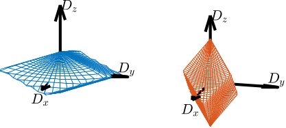
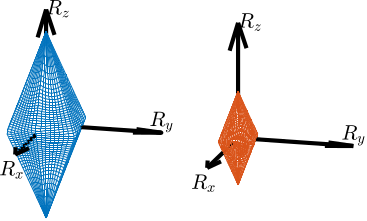
To better understand how the geometry of the Stewart platform impacts the translational mobility, two configurations are compared:

• Struts oriented horizontally (Figure ref:fig:detail_kinematics_stewart_mobility_vert_struts) => more stroke in horizontal direction
• Struts oriented vertically (Figure ref:fig:detail_kinematics_stewart_mobility_hori_struts) => more stroke in vertical direction
• Corresponding mobility shown in Figure ref:fig:detail_kinematics_mobility_translation_strut_orientation

\bigskip

Mobility in rotation

As shown by equation eqref:eq:detail_kinematics_jacobian, the rotational mobility depends both on the orientation of the struts and on the location of the top joints.

Similarly to the translational case, to increase the rotational mobility in one direction, it is advantageous to have the struts more perpendicular to the rotational direction.

For instance, having the struts more vertical (Figure ref:fig:detail_kinematics_stewart_mobility_vert_struts) gives less rotational stroke along the vertical direction than having the struts oriented more horizontally (Figure ref:fig:detail_kinematics_stewart_mobility_hori_struts).

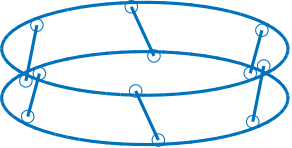
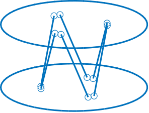
Two cases are considered with same strut orientation but with different top joints positions:

• struts close to each other (Figure ref:fig:detail_kinematics_stewart_mobility_close_struts)
• struts further apart (Figure ref:fig:detail_kinematics_stewart_mobility_space_struts)

The mobility for pure rotations are compared in Figure ref:fig:detail_kinematics_mobility_angle_strut_distance. Note that the same strut stroke are considered in both cases to evaluate the mobility. Having struts further apart decreases the "level arm" and therefore the rotational mobility is reduced.

For rotations and translations, having more mobility also means increasing the effect of actuator noise on the considering degree of freedom. Somehow, the level arm is increased, so any strut vibration gets amplified. Therefore, the designed Stewart platform should just have the necessary mobility.

\bigskip

Combined translations and rotations

It is possible to consider combined translations and rotations. Displaying such mobility is more complex. It will be used for the nano-hexapod to verify that the obtained design has the necessary mobility.

For a fixed geometry and a wanted mobility (combined translations and rotations), it is possible to estimate the required minimum actuator stroke. It will be done in Section ref:sec:detail_kinematics_nano_hexapod to estimate the required actuator stroke for the nano-hexapod geometry.

Stiffness

Introduction   ignore

Stiffness matrix:

• defines how the nano-hexapod deforms (frame $\{B\}$ with respect to frame $\{A\}$) due to static forces/torques applied on $\{B\}$.
• Depends on the Jacobian matrix (i.e. the geometry) and the strut axial stiffness eqref:eq:detail_kinematics_stiffness_matrix
• Contribution of joints stiffness is here not considered cite:&mcinroy00_desig_contr_flexur_joint_hexap;&mcinroy02_model_desig_flexur_joint_stewar

\begin{equation}\label{eq:detail_kinematics_stiffness_matrix} \bm{K} = \bm{J}^T \bm{\mathcal{K}} \bm{J}

\end{equation}

It is assumed that the stiffness of all strut is the same: $\bm{\mathcal{K}} = k \cdot \mathbf{I}_6$. Obtained stiffness matrix linearly depends on the strut stiffness $k$ eqref:eq:detail_kinematics_stiffness_matrix_simplified.

\begin{equation}\label{eq:detail_kinematics_stiffness_matrix_simplified} \bm{K} = k \bm{J}^T \bm{J} = k ≤ft[ \begin{array}{c|c} Σ_{i = 0}⁶ \hat{\bm{s}}_i ⋅ \hat{\bm{s}}_i^T & Σ_{i = 0}⁶ \bm{\hat{s}}_i ⋅ ({}^A\bm{b}_i × {}^A\hat{\bm{s}}_i)^T
\hline Σ_{i = 0}⁶ ({}^A\bm{b}_i × {}^A\hat{\bm{s}}_i) ⋅ \hat{\bm{s}}_i^T & Σ_{i = 0}⁶ ({}^A\bm{b}_i × {}^A\hat{\bm{s}}_i) ⋅ ({}^A\bm{b}_i × {}^A\hat{\bm{s}}_i)^T\\

\end{array} \right]

\end{equation}

Translation Stiffness

XYZ stiffnesses:

• Only depends on the orientation of the struts and not their location: $\hat{\bm{s}}_i \cdot \hat{\bm{s}}_i^T$
• Extreme case: all struts are vertical $s_i = [0,\ 0,\ 1]$ => vertical stiffness of $6 k$, but null stiffness in X and Y directions
• If two struts along X, two struts along Y, and two struts along Z => $\hat{\bm{s}}_i \cdot \hat{\bm{s}}_i^T = 2 \bm{I}_3$ Stiffness is well distributed along directions. This corresponds to the cubic architecture.

If struts more vertical (Figure ref:fig:detail_kinematics_stewart_mobility_vert_struts):

• increase vertical stiffness
• decrease horizontal stiffness
• increase Rx,Ry stiffness
• decrease Rz stiffness

Opposite conclusions if struts are not horizontal (Figure ref:fig:detail_kinematics_stewart_mobility_hori_struts).

Rotational Stiffness

Rotational stiffnesses:

• Same orientation but increased distances (bi) by a factor 2 => rotational stiffness increased by factor 4 Figure ref:fig:detail_kinematics_stewart_mobility_close_struts Figure ref:fig:detail_kinematics_stewart_mobility_space_struts

Struts further apart:

• no change to XYZ
• increase in rotational stiffness (by the square of the distance)

Diagonal Stiffness Matrix

Having the stiffness matrix $\bm{K}$ diagonal can be beneficial for control purposes as it would make the plant in the cartesian frame decoupled at low frequency.

This depends on the geometry and on the chosen {A} frame.

For specific configurations, it is possible to have a diagonal K matrix.

Dynamical properties

In the Cartesian Frame

Dynamical equations (both in the cartesian frame and in the frame of the struts) for the Stewart platform were derived during the conceptual phase with simplifying assumptions (massless struts and perfect joints).

The dynamics depends both on the geometry (Jacobian matrix) but also on the payload being placed on top of the platform.

Under very specific conditions, the equations of motion can be decoupled in the Cartesian space. These are studied in Section ref:ssec:detail_kinematics_cubic_dynamic.

\begin{equation}\label{eq:nhexa_transfer_function_cart} \frac{{\mathcal{X}}}{\bm{\mathcal{F}}}(s) = ( \bm{M} s^2 + \bm{J}^T \bm{\mathcal{C}} \bm{J} s + \bm{J}^T \bm{\mathcal{K}} \bm{J} )^-1

\end{equation}

In the frame of the Struts

In the frame of the struts, the equations of motion are well decoupled at low frequency. This is why most of Stewart platforms are controlled in the frame of the struts: bellow the resonance frequency, the system is decoupled and SISO control may be applied for each strut.

\begin{equation}\label{eq:nhexa_transfer_function_struts} \frac{\bm{\mathcal{L}}}{\bm{f}}(s) = ( \bm{J}^-T \bm{M} \bm{J}^-1 s^2 + \bm{\mathcal{C}} + \bm{\mathcal{K}} )^-1

\end{equation}

Coupling between sensors (force sensors, relative position sensor, inertial sensors) in different struts may also be important for decentralized control. Can the geometry be optimized to have lower coupling between the struts? This will be studied with the cubic architecture.

TODO Dynamic Isotropy

cite:&afzali-far16_vibrat_dynam_isotr_hexap_analy_studies: "Dynamic isotropy, leading to equal eigenfrequencies, is a powerful optimization measure."

Conclusion

The effects of two changes in the manipulator's geometry, namely the position and orientation of the legs, are summarized in Table ref:tab:detail_kinematics_geometry. These results could have been easily deduced based on some mechanical principles, but thanks to the kinematic analysis, they can be quantified.

These trade-offs give some guidelines when choosing the Stewart platform geometry.

	legs pointing more vertically	legs further apart
Vertical stiffness	$\nearrow$	$=$
Horizontal stiffness	$\searrow$	$=$
Vertical rotation stiffness	$\searrow$	$\nearrow$
Horizontal rotation stiffness	$\nearrow$	$\nearrow$
Vertical force authority	$\nearrow$	$=$
Horizontal force authority	$\searrow$	$=$
Vertical torque authority	$\searrow$	$\nearrow$
Horizontal torque authority	$\nearrow$	$\nearrow$
Vertical stroke	$\searrow$	$=$
Horizontal stroke	$\nearrow$	$=$
Vertical rotation stroke	$\nearrow$	$\searrow$
Horizontal rotation stroke	$\searrow$	$\searrow$

Effect of a change in geometry on the manipulator's stiffness, force authority and stroke

The Cubic Architecture

<<sec:detail_kinematics_cubic>>

Introduction   ignore

The Cubic configuration for the Stewart platform was first proposed in cite:&geng94_six_degree_of_freed_activ.

This configuration is quite specific in the sense that the active struts are arranged in a mutually orthogonal configuration connecting the corners of a cube Figure ref:fig:detail_kinematics_cubic_schematic.

Cubic configuration:

• The struts are corresponding to 6 of the 8 edges of a cube.
• This way, all struts are perpendicular to each other (except sets of two that are parallel).

  \begin{tikzpicture}
    \begin{scope}[rotate={45}, shift={(0, 0, -4)}]
      % We first define the coordinate of the points of the Cube
      \coordinate[] (bot) at (0,0,4);
      \coordinate[] (top) at (4,4,0);
      \coordinate[] (A1) at (0,0,0);
      \coordinate[] (A2) at (4,0,4);
      \coordinate[] (A3) at (0,4,4);
      \coordinate[] (B1) at (4,0,0);
      \coordinate[] (B2) at (4,4,4);
      \coordinate[] (B3) at (0,4,0);

      % Center of the Cube
      \node[] (cubecenter) at ($0.5*(bot) + 0.5*(top)$){$\bullet$};
      % \node[above right] at (cubecenter){$C$};

      % We draw parts of the cube that corresponds to the Stewart platform
      \draw[] (A1)node[]{$\bullet$} -- (B1)node[]{$\bullet$} -- (A2)node[]{$\bullet$} -- (B2)node[]{$\bullet$} -- (A3)node[]{$\bullet$} -- (B3)node[]{$\bullet$} -- (A1);
      \draw[opacity=0.5] (bot) -- (A1);
      \draw[opacity=0.5] (bot) -- (A2);
      \draw[opacity=0.5] (bot) -- (A3);
      \draw[opacity=0.5] (top) -- (B1);
      \draw[opacity=0.5] (top) -- (B2);
      \draw[opacity=0.5] (top) -- (B3);

      % ai and bi are computed
      \def\lfrom{0.1}
      \def\lto{0.9}

      \coordinate(a1) at ($(A1) - \lfrom*(A1) + \lfrom*(B1)$);
      \coordinate(b1) at ($(A1) - \lto*(A1)   + \lto*(B1)$);
      \coordinate(a2) at ($(A2) - \lfrom*(A2) + \lfrom*(B1)$);
      \coordinate(b2) at ($(A2) - \lto*(A2)   + \lto*(B1)$);
      \coordinate(a3) at ($(A2) - \lfrom*(A2) + \lfrom*(B2)$);
      \coordinate(b3) at ($(A2) - \lto*(A2)   + \lto*(B2)$);
      \coordinate(a4) at ($(A3) - \lfrom*(A3) + \lfrom*(B2)$);
      \coordinate(b4) at ($(A3) - \lto*(A3)   + \lto*(B2)$);
      \coordinate(a5) at ($(A3) - \lfrom*(A3) + \lfrom*(B3)$);
      \coordinate(b5) at ($(A3) - \lto*(A3)   + \lto*(B3)$);
      \coordinate(a6) at ($(A1) - \lfrom*(A1) + \lfrom*(B3)$);
      \coordinate(b6) at ($(A1) - \lto*(A1)   + \lto*(B3)$);

      % Center of the Stewart Platform
      % \node[color=colorblue] at ($0.25*(a1) + 0.25*(a6) + 0.25*(b3) + 0.25*(b4)$){$\bullet$};

      % We draw the fixed and mobiles platforms
      \path[fill=colorblue, opacity=0.2] (a1) -- (a2) -- (a3) -- (a4) -- (a5) -- (a6) -- cycle;
      \path[fill=colorblue, opacity=0.2] (b1) -- (b2) -- (b3) -- (b4) -- (b5) -- (b6) -- cycle;
      \draw[color=colorblue, dashed] (a1) -- (a2) -- (a3) -- (a4) -- (a5) -- (a6) -- cycle;
      \draw[color=colorblue, dashed] (b1) -- (b2) -- (b3) -- (b4) -- (b5) -- (b6) -- cycle;

      % The legs of the hexapod are drawn
      \draw[color=colorblue] (a1)node{$\bullet$} -- (b1)node{$\bullet$};
      \draw[color=colorblue] (a2)node{$\bullet$} -- (b2)node{$\bullet$};
      \draw[color=colorblue] (a3)node{$\bullet$} -- (b3)node{$\bullet$};
      \draw[color=colorblue] (a4)node{$\bullet$} -- (b4)node{$\bullet$};
      \draw[color=colorblue] (a5)node{$\bullet$} -- (b5)node{$\bullet$};
      \draw[color=colorblue] (a6)node{$\bullet$} -- (b6)node{$\bullet$};
    \end{scope}

    % Height of the Hexapod
    \coordinate[] (sizepos) at ($(a2)+(0.2, 0)$);
    \coordinate[] (origin) at (0,0,0);
    % \draw[<->, dashed] (a2-|sizepos) -- node[midway, right]{$H$} (b2-|sizepos);
    % Height offset
    % \draw[<->, dashed] (a2-|sizepos) -- node[midway, right]{$H_0$} (origin-|sizepos);

    % \draw[<->, dashed] (0.5,2,0) --node[near end, right]{${}^{F}O_{C}$} ++(0,2,0);
    % \draw[<->, dashed] (-2,2,0) --node[midway, right]{${}^{F}H_{A}$} ++(0,1,0);
    % \draw[<->, dashed] (-2,6,0) --node[midway, right]{${}^{M}H_{B}$} ++(0,-1.5,0);

    % Useful part of the cube
    % \draw[<->, dashed] ($(A2)+(0.5,0)$) -- node[midway, right]{$H_{C}$} ($(B1)+(0.5,0)$);
  \end{tikzpicture}

Stewart platform Cubic architecture. The struts are aligned with the sides of a cube.

The cubic configuration is attributed a number of properties that made this configuration widely used (cite:&preumont07_six_axis_singl_stage_activ;&jafari03_orthog_gough_stewar_platf_microm). From cite:&geng94_six_degree_of_freed_activ:

1. Uniformity in control capability in all directions
2. Uniformity in stiffness in all directions
3. Minimum cross coupling force effect among actuators
4. Facilitate collocated sensor-actuator control system design
5. Simple kinematics relationships
6. Simple dynamic analysis
7. Simple mechanical design

According to cite:&preumont07_six_axis_singl_stage_activ, it "minimizes the cross-coupling amongst actuators and sensors of different legs" (being orthogonal to each other).

Specific points of interest are:

• uniform mobility, uniform stiffness, and coupling properties

In this section:

• Such properties are studied
• Additional properties interesting for control?
• It is determined if the cubic architecture is interested for the nano-hexapod

The Cubic Architecture

<<ssec:detail_kinematics_cubic_presentation>>

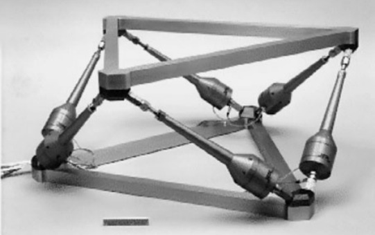
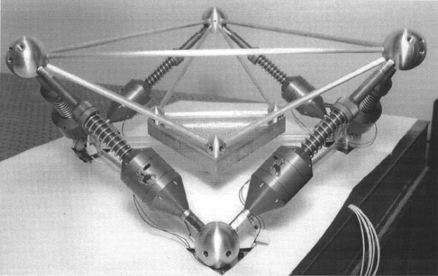
Typical cubic architecture (Figure ref:fig:detail_kinematics_cubic_architecture_examples).

Struts with similar size than the cube's edge (Figure ref:fig:detail_kinematics_cubic_architecture_example). Similar to Figures ref:fig:detail_kinematics_jpl, ref:fig:detail_kinematics_uw_gsp and ref:fig:detail_kinematics_uqp.

Struts smaller than the cube's edge (Figure ref:fig:detail_kinematics_cubic_architecture_example_small). Similar to the Stewart platform of Figure ref:fig:detail_kinematics_ulb_pz.

The two stewart platform are having the same properties (stiffness matrix, when evaluated at the cube's center).

Static Properties

<<ssec:detail_kinematics_cubic_static>>

Uniform stiffness

First, we have to understand what is the physical meaning of the Stiffness matrix $\bm{K}$.

The Stiffness matrix links forces $\bm{f}$ and torques $\bm{n}$ applied on the mobile platform at $\{B\}$ to the displacement $\Delta\bm{\mathcal{X}}$ of the mobile platform represented by $\{B\}$ with respect to $\{A\}$: \[ \bm{\mathcal{F}} = \bm{K} \Delta\bm{\mathcal{X}} \]

with:

• $\bm{\mathcal{F}} = [\bm{f}\ \bm{n}]^{T}$
• $\Delta\bm{\mathcal{X}} = [\delta x, \delta y, \delta z, \delta \theta_{x}, \delta \theta_{y}, \delta \theta_{z}]^{T}$

If the stiffness matrix is inversible, its inverse is the compliance matrix: $\bm{C} = \bm{K}^{-1$ and: \[ \Delta \bm{\mathcal{X}} = C \bm{\mathcal{F}} \]

Thus, if the stiffness matrix is diagonal, the compliance matrix is also diagonal and a force (resp. torque) $\bm{\mathcal{F}}_i$ applied on the mobile platform at $\{B\}$ will induce a pure translation (resp. rotation) of the mobile platform represented by $\{B\}$ with respect to $\{A\}$.

• Frames at the center of the cube => diagonal K matrix => static decoupling in the cartesian frame (show the control architecture?)
• Frames above the top platform => non-diagonal K matrix => coupled at low frequency
• Uniform stiffness in X,Y,Z, equal to two times the actuator stiffness Krx = Kry, but not equal to Krz
• Jacobian matrix? Any special?

The cubic architecture has indeed identical translational stiffnesses.

Therefore, the cubic architecture is special only when considering a frame located at the center of the cube. This is not very convenient, as in the vast majority of cases, the interesting frame is located about the top platform.

• Get the analytical formula for the Stiffness matrix?

2.0	0.0	-0.0	-0.0	0.0	-0.0
0.0	2.0	-0.0	-0.0	-0.0	-0.0
-0.0	-0.0	2.0	-0.0	0.0	0.0
-0.0	-0.0	-0.0	0.015	-0.0	0.0
0.0	-0.0	0.0	-0.0	0.015	-0.0
-0.0	-0.0	0.0	0.0	-0.0	0.06

2.0	-0.0	-0.0	0.0	-0.2	0.0
-0.0	2.0	0.0	0.2	-0.0	0.0
-0.0	0.0	2.0	-0.0	0.0	0.0
0.0	0.2	-0.0	0.035	-0.0	0.0
-0.2	-0.0	0.0	-0.0	0.035	0.0
0.0	0.0	0.0	0.0	0.0	0.06

Note that the cube's center needs not to be at the "center" of the Stewart platform. This can lead to interesting architectures shown in Section ref:ssec:detail_kinematics_cubic_design.

Here are the conclusion about the Stiffness matrix for the Cubic configuration:

• The cubic configuration permits to have $k_x = k_y = k_z$ and $k_{\theta_x} = k_{\theta_y}$
• The stiffness matrix $K$ is diagonal for the cubic configuration if the Jacobian is estimated at the cube center

Uniform Mobility

Uniform mobility in X,Y,Z directions

Show that be obtain a cube.

Cubic configuration: "Vertical cube" with

%% With cubic configuration
H = 100e-3;     % Height of the Stewart platform [m]
Hc = 100e-3;   % Size of the useful part of the cube [m]
FOc = 50e-3; % Center of the cube at the Stewart platform center
MO_B = -50e-3;  % Position {B} with respect to {M} [m]
MHb = 0;

stewart_cubic = initializeStewartPlatform();
stewart_cubic = initializeFramesPositions(stewart_cubic, 'H', H, 'MO_B', MO_B);
stewart_cubic = generateCubicConfiguration(stewart_cubic, 'Hc', Hc, 'FOc', FOc, 'FHa', 5e-3, 'MHb', MHb);
stewart_cubic = computeJointsPose(stewart_cubic);
stewart_cubic = initializeStrutDynamics(stewart_cubic, 'k', 1);
stewart_cubic = computeJacobian(stewart_cubic);
stewart_cubic = initializeCylindricalPlatforms(stewart_cubic, 'Fpr', 150e-3, 'Mpr', 150e-3);

% Let's now define the actuator stroke.
L_max =  50e-6; % [m]

thetas = linspace(0, pi, 100);
phis = linspace(0, 2*pi, 200);
rs = zeros(length(thetas), length(phis));

for i = 1:length(thetas)
    for j = 1:length(phis)
        Tx = sin(thetas(i))*cos(phis(j));
        Ty = sin(thetas(i))*sin(phis(j));
        Tz = cos(thetas(i));

        dL = stewart_cubic.kinematics.J*[Tx; Ty; Tz; 0; 0; 0;]; % dL required for 1m displacement in theta/phi direction

        rs(i, j) = L_max/max(abs(dL));
        % rs(i, j) = max(abs([dL(dL<0)*L_min; dL(dL>=0)*L_max]));
    end
end

% Get circle that fits inside the accessible space
min(min(rs))
max(max(rs))

[phi_grid, theta_grid] = meshgrid(phis, thetas);
X = 1e6 * rs .* sin(theta_grid) .* cos(phi_grid);
Y = 1e6 * rs .* sin(theta_grid) .* sin(phi_grid);
Z = 1e6 * rs .* cos(theta_grid);

figure;
s = surf(X, Y, Z, 'FaceColor', 'white');
s.EdgeColor = colors(1,:);
axis equal;
grid on;
xlabel('X Translation [$\mu$m]'); ylabel('Y Translation [$\mu$m]'); zlabel('Z Translation [$\mu$m]');
xlim(5e6*[-L_max, L_max]); ylim(5e6*[-L_max, L_max]); zlim(5e6*[-L_max, L_max]);

Dynamical Decoupling

<<ssec:detail_kinematics_cubic_dynamic>>

Introduction   ignore

cite:&mcinroy00_desig_contr_flexur_joint_hexap

In this section, we study the dynamics of the platform in the cartesian frame.

We here suppose that there is one relative motion sensor in each strut ($\delta\bm{\mathcal{L}}$ is measured) and we would like to control the position of the top platform pose $\delta \bm{\mathcal{X}}$.

Thanks to the Jacobian matrix, we can use the "architecture" shown in Figure ref:fig:detail_kinematics_local_to_cartesian_coordinates to obtain the dynamics of the system from forces/torques applied by the actuators on the top platform to translations/rotations of the top platform.

\begin{tikzpicture}
  \node[block] (Jt) at (0, 0) {$\bm{J}^{-T}$};
  \node[block, right= of Jt] (G) {$\bm{G}$};
  \node[block, right= of G] (J) {$\bm{J}^{-1}$};

  \draw[->] ($(Jt.west)+(-0.8, 0)$) -- (Jt.west) node[above left]{$\bm{\mathcal{F}}$};
  \draw[->] (Jt.east) -- (G.west) node[above left]{$\bm{\tau}$};
  \draw[->] (G.east) -- (J.west) node[above left]{$\delta\bm{\mathcal{L}}$};
  \draw[->] (J.east) -- ++(0.8, 0) node[above left]{$\delta\bm{\mathcal{X}}$};
\end{tikzpicture}

From Strut coordinate to Cartesian coordinate using the Jacobian matrix

We here study the dynamics from $\bm{\mathcal{F}}$ to $\delta\bm{\mathcal{X}}$.

One has to note that when considering the static behavior: \[ \bm{G}(s = 0) = \begin{bmatrix} 1/k_1 & & 0 \\ & \ddots & 0 \\ 0 & & 1/k_6 \end{bmatrix}\]

And thus: \[ \frac{\delta\bm{\mathcal{X}}}{\bm{\mathcal{F}}}(s = 0) = \bm{J}^{-1} \bm{G}(s = 0) \bm{J}^{-T} = \bm{K}^{-1} = \bm{C} \]

We conclude that the static behavior of the platform depends on the stiffness matrix. For the cubic configuration, we have a diagonal stiffness matrix is the frames $\{A\}$ and $\{B\}$ are coincident with the cube's center.

Cube's center at the Center of Mass of the mobile platform

Let's create a Cubic Stewart Platform where the Center of Mass of the mobile platform is located at the center of the cube.

We define the size of the Stewart platform and the position of frames $\{A\}$ and $\{B\}$.

H    = 200e-3; % height of the Stewart platform [m]
MO_B = -10e-3;  % Position {B} with respect to {M} [m]

Now, we set the cube's parameters such that the center of the cube is coincident with $\{A\}$ and $\{B\}$.

Hc   = 2.5*H;    % Size of the useful part of the cube [m]
FOc  = H + MO_B; % Center of the cube with respect to {F}

stewart = initializeStewartPlatform();
stewart = initializeFramesPositions(stewart, 'H', H, 'MO_B', MO_B);
stewart = generateCubicConfiguration(stewart, 'Hc', Hc, 'FOc', FOc, 'FHa', 25e-3, 'MHb', 25e-3);
stewart = computeJointsPose(stewart);
stewart = initializeStrutDynamics(stewart, 'k', 1e6, 'c', 1e1);
stewart = initializeJointDynamics(stewart, 'type_F', 'universal', 'type_M', 'spherical');
stewart = computeJacobian(stewart);
stewart = initializeStewartPose(stewart);

Now we set the geometry and mass of the mobile platform such that its center of mass is coincident with $\{A\}$ and $\{B\}$.

stewart = initializeCylindricalPlatforms(stewart, 'Fpr', 1.2*max(vecnorm(stewart.platform_F.Fa)), ...
                                         'Mpm', 10, ...
                                         'Mph', 20e-3, ...
                                         'Mpr', 1.2*max(vecnorm(stewart.platform_M.Mb)));

And we set small mass for the struts.

stewart = initializeCylindricalStruts(stewart, 'Fsm', 1e-3, 'Msm', 1e-3);
stewart = initializeInertialSensor(stewart);

No flexibility below the Stewart platform and no payload.

ground = initializeGround('type', 'none');
payload = initializePayload('type', 'none');
controller = initializeController('type', 'open-loop');

The obtain geometry is shown in figure fig:stewart_cubic_conf_decouple_dynamics.

<<plt-matlab>>

Geometry used for the simulations - The cube's center, the frames $\{A\}$ and $\{B\}$ and the Center of mass of the mobile platform are coincident (png, pdf)

We now identify the dynamics from forces applied in each strut $\bm{\tau}$ to the displacement of each strut $d \bm{\mathcal{L}}$.

open('stewart_platform_model.slx')

%% Options for Linearized
options = linearizeOptions;
options.SampleTime = 0;

%% Name of the Simulink File
mdl = 'stewart_platform_model';

%% Input/Output definition
clear io; io_i = 1;
io(io_i) = linio([mdl, '/Controller'],        1, 'openinput');  io_i = io_i + 1; % Actuator Force Inputs [N]
io(io_i) = linio([mdl, '/Stewart Platform'],  1, 'openoutput', [], 'dLm'); io_i = io_i + 1; % Relative Displacement Outputs [m]

%% Run the linearization
G = linearize(mdl, io, options);
G.InputName  = {'F1', 'F2', 'F3', 'F4', 'F5', 'F6'};
G.OutputName = {'Dm1', 'Dm2', 'Dm3', 'Dm4', 'Dm5', 'Dm6'};

Now, thanks to the Jacobian (Figure fig:local_to_cartesian_coordinates), we compute the transfer function from $\bm{\mathcal{F}}$ to $\bm{\mathcal{X}}$.

Gc = inv(stewart.kinematics.J)*G*inv(stewart.kinematics.J');
Gc = inv(stewart.kinematics.J)*G*stewart.kinematics.J;
Gc.InputName  = {'Fx', 'Fy', 'Fz', 'Mx', 'My', 'Mz'};
Gc.OutputName = {'Dx', 'Dy', 'Dz', 'Rx', 'Ry', 'Rz'};

The obtain dynamics $\bm{G}_{c}(s) = \bm{J}^{-T} \bm{G}(s) \bm{J}^{-1}$ is shown in Figure fig:stewart_cubic_decoupled_dynamics_cartesian.

<<plt-matlab>>

Dynamics from $\bm{\mathcal{F}}$ to $\bm{\mathcal{X}}$ (png, pdf)

It is interesting to note here that the system shown in Figure fig:local_to_cartesian_coordinates_bis also yield a decoupled system (explained in section 1.3.3 in cite:li01_simul_fault_vibrat_isolat_point).

\begin{tikzpicture}
  \node[block] (Jt) at (0, 0) {$\bm{J}$};
  \node[block, right= of Jt] (G) {$\bm{G}$};
  \node[block, right= of G] (J) {$\bm{J}^{-1}$};

  \draw[->] ($(Jt.west)+(-0.8, 0)$) -- (Jt.west);
  \draw[->] (Jt.east) -- (G.west) node[above left]{$\bm{\tau}$};
  \draw[->] (G.east) -- (J.west) node[above left]{$\delta\bm{\mathcal{L}}$};
  \draw[->] (J.east) -- ++(0.8, 0) node[above left]{$\delta\bm{\mathcal{X}}$};
\end{tikzpicture}

Alternative way to decouple the system

The dynamics is well decoupled at all frequencies.

We have the same dynamics for:

• $D_x/F_x$, $D_y/F_y$ and $D_z/F_z$
• $R_x/M_x$ and $D_y/F_y$

The Dynamics from $F_i$ to $D_i$ is just a 1-dof mass-spring-damper system.

This is because the Mass, Damping and Stiffness matrices are all diagonal.

Cube's center not coincident with the Mass of the Mobile platform

Let's create a Stewart platform with a cubic architecture where the cube's center is at the center of the Stewart platform.

H    = 200e-3; % height of the Stewart platform [m]
MO_B = -100e-3;  % Position {B} with respect to {M} [m]

Now, we set the cube's parameters such that the center of the cube is coincident with $\{A\}$ and $\{B\}$.

Hc   = 2.5*H;    % Size of the useful part of the cube [m]
FOc  = H + MO_B; % Center of the cube with respect to {F}

stewart = initializeStewartPlatform();
stewart = initializeFramesPositions(stewart, 'H', H, 'MO_B', MO_B);
stewart = generateCubicConfiguration(stewart, 'Hc', Hc, 'FOc', FOc, 'FHa', 25e-3, 'MHb', 25e-3);
stewart = computeJointsPose(stewart);
stewart = initializeStrutDynamics(stewart, 'K', 1e6*ones(6,1), 'C', 1e1*ones(6,1));
stewart = initializeJointDynamics(stewart, 'type_F', 'universal', 'type_M', 'spherical');
stewart = computeJacobian(stewart);
stewart = initializeStewartPose(stewart);

However, the Center of Mass of the mobile platform is not located at the cube's center.

stewart = initializeCylindricalPlatforms(stewart, 'Fpr', 1.2*max(vecnorm(stewart.platform_F.Fa)), ...
                                         'Mpm', 10, ...
                                         'Mph', 20e-3, ...
                                         'Mpr', 1.2*max(vecnorm(stewart.platform_M.Mb)));

And we set small mass for the struts.

stewart = initializeCylindricalStruts(stewart, 'Fsm', 1e-3, 'Msm', 1e-3);
stewart = initializeInertialSensor(stewart);

No flexibility below the Stewart platform and no payload.

ground = initializeGround('type', 'none');
payload = initializePayload('type', 'none');
controller = initializeController('type', 'open-loop');

The obtain geometry is shown in figure fig:stewart_cubic_conf_mass_above.

<<plt-matlab>>

Geometry used for the simulations - The cube's center is coincident with the frames $\{A\}$ and $\{B\}$ but not with the Center of mass of the mobile platform (png, pdf)

We now identify the dynamics from forces applied in each strut $\bm{\tau}$ to the displacement of each strut $d \bm{\mathcal{L}}$.

open('stewart_platform_model.slx')

%% Options for Linearized
options = linearizeOptions;
options.SampleTime = 0;

%% Name of the Simulink File
mdl = 'stewart_platform_model';

%% Input/Output definition
clear io; io_i = 1;
io(io_i) = linio([mdl, '/Controller'],        1, 'openinput');  io_i = io_i + 1; % Actuator Force Inputs [N]
io(io_i) = linio([mdl, '/Stewart Platform'],  1, 'openoutput', [], 'dLm'); io_i = io_i + 1; % Relative Displacement Outputs [m]

%% Run the linearization
G = linearize(mdl, io, options);
G.InputName  = {'F1', 'F2', 'F3', 'F4', 'F5', 'F6'};
G.OutputName = {'Dm1', 'Dm2', 'Dm3', 'Dm4', 'Dm5', 'Dm6'};

And we use the Jacobian to compute the transfer function from $\bm{\mathcal{F}}$ to $\bm{\mathcal{X}}$.

Gc = inv(stewart.kinematics.J)*G*inv(stewart.kinematics.J');
Gc.InputName  = {'Fx', 'Fy', 'Fz', 'Mx', 'My', 'Mz'};
Gc.OutputName = {'Dx', 'Dy', 'Dz', 'Rx', 'Ry', 'Rz'};

The obtain dynamics $\bm{G}_{c}(s) = \bm{J}^{-T} \bm{G}(s) \bm{J}^{-1}$ is shown in Figure fig:stewart_conf_coupling_mass_matrix.

<<plt-matlab>>

Obtained Dynamics from $\bm{\mathcal{F}}$ to $\bm{\mathcal{X}}$ (png, pdf)

The system is decoupled at low frequency (the Stiffness matrix being diagonal), but it is not decoupled at all frequencies.

This was expected as the mass matrix is not diagonal (the Center of Mass of the mobile platform not being coincident with the frame $\{B\}$).

Dynamic isotropy

cite:&afzali-far16_vibrat_dynam_isotr_hexap_analy_studies:

• proposes an architecture where the CoM can be above the top platform
• Try to find a stewart platform an a payload for witch all resonances are equal. Massless struts and plates. Cylindrical payload tuned to obtained such property. Show that all modes can be optimally damped? Compare with Stewart platform with different resonance frequencies. Also need to have parallel stiffness with the struts
• Same resonance frequencies for suspension modes? Maybe in one case: sphere at the CoM? Could be nice to show that. Say that this can be nice for optimal damping for instance (link to paper explaining that)

• Show examples where the dynamics can indeed be decoupled in the cartesian frame (i.e. decoupled K and M matrices)

Conclusion

• Better decoupling between the struts? Next section

Some conclusions can be drawn from the above analysis:

• Static Decoupling <=> Diagonal Stiffness matrix <=> {A} and {B} at the cube's center
• Dynamic Decoupling <=> Static Decoupling + CoM of mobile platform coincident with {A} and {B}.

TODO Decentralized Control

Introduction   ignore

From cite:preumont07_six_axis_singl_stage_activ, the cubic configuration "minimizes the cross-coupling amongst actuators and sensors of different legs (being orthogonal to each other)".

This would facilitate the use of decentralized control.

In this section, we wish to study such properties of the cubic architecture.

We will compare the transfer function from sensors to actuators in each strut for a cubic architecture and for a non-cubic architecture (where the struts are not orthogonal with each other).

Cubic Architecture

Let's generate a Cubic architecture where the cube's center and the frames $\{A\}$ and $\{B\}$ are coincident.

H    = 200e-3; % height of the Stewart platform [m]
MO_B = -10e-3;  % Position {B} with respect to {M} [m]
Hc   = 2.5*H;    % Size of the useful part of the cube [m]
FOc  = H + MO_B; % Center of the cube with respect to {F}

stewart = initializeStewartPlatform();
stewart = initializeFramesPositions(stewart, 'H', H, 'MO_B', MO_B);
stewart = generateCubicConfiguration(stewart, 'Hc', Hc, 'FOc', FOc, 'FHa', 25e-3, 'MHb', 25e-3);
stewart = computeJointsPose(stewart);
stewart = initializeStrutDynamics(stewart, 'k', 1e6, 'c', 1e1);
stewart = initializeJointDynamics(stewart, 'type_F', 'universal', 'type_M', 'spherical');
stewart = computeJacobian(stewart);
stewart = initializeStewartPose(stewart);
stewart = initializeCylindricalPlatforms(stewart, 'Fpr', 1.2*max(vecnorm(stewart.platform_F.Fa)), ...
                                         'Mpm', 10, ...
                                         'Mph', 20e-3, ...
                                         'Mpr', 1.2*max(vecnorm(stewart.platform_M.Mb)));
stewart = initializeCylindricalStruts(stewart, 'Fsm', 1e-3, 'Msm', 1e-3);
stewart = initializeInertialSensor(stewart);

No flexibility below the Stewart platform and no payload.

ground = initializeGround('type', 'none');
payload = initializePayload('type', 'none');
controller = initializeController('type', 'open-loop');

disturbances = initializeDisturbances();
references = initializeReferences(stewart);

And we identify the dynamics from the actuator forces $\tau_{i}$ to the relative motion sensors $\delta \mathcal{L}_{i}$ (Figure fig:coupling_struts_relative_sensor_cubic) and to the force sensors $\tau_{m,i}$ (Figure fig:coupling_struts_force_sensor_cubic).

Non-Cubic Architecture

Now we generate a Stewart platform which is not cubic but with approximately the same size as the previous cubic architecture.

H    = 200e-3; % height of the Stewart platform [m]
MO_B = -10e-3;  % Position {B} with respect to {M} [m]

stewart = initializeStewartPlatform();
stewart = initializeFramesPositions(stewart, 'H', H, 'MO_B', MO_B);
stewart = generateGeneralConfiguration(stewart, 'FR', 250e-3, 'MR', 150e-3);
stewart = computeJointsPose(stewart);
stewart = initializeStrutDynamics(stewart, 'k', 1e6, 'c', 1e1);
stewart = initializeJointDynamics(stewart, 'type_F', 'universal', 'type_M', 'spherical');
stewart = computeJacobian(stewart);
stewart = initializeStewartPose(stewart);
stewart = initializeCylindricalPlatforms(stewart, 'Fpr', 1.2*max(vecnorm(stewart.platform_F.Fa)), ...
                                         'Mpm', 10, ...
                                         'Mph', 20e-3, ...
                                         'Mpr', 1.2*max(vecnorm(stewart.platform_M.Mb)));
stewart = initializeCylindricalStruts(stewart, 'Fsm', 1e-3, 'Msm', 1e-3);
stewart = initializeInertialSensor(stewart);

No flexibility below the Stewart platform and no payload.

ground = initializeGround('type', 'none');
payload = initializePayload('type', 'none');
controller = initializeController('type', 'open-loop');

And we identify the dynamics from the actuator forces $\tau_{i}$ to the relative motion sensors $\delta \mathcal{L}_{i}$ (Figure fig:coupling_struts_relative_sensor_non_cubic) and to the force sensors $\tau_{m,i}$ (Figure fig:coupling_struts_force_sensor_non_cubic).

Conclusion

The Cubic architecture seems to not have any significant effect on the coupling between actuator and sensors of each strut and thus provides no advantages for decentralized control.

Cubic architecture with Cube's center above the top platform

<<ssec:detail_kinematics_cubic_design>>

Introduction   ignore

We saw in section ref:ssec:detail_kinematics_cubic_static that in order to have a diagonal stiffness matrix, the cube's center needs to be located at frames $\{A\}$ and $\{B\}$. Or, typically $\{A\}$ and $\{B\}$ are located above the top platform where forces are applied and where displacements are expressed.

Say a 100mm tall Stewart platform needs to be designed with the CoM of the payload 20mm above the top platform. The cube's center therefore needs to be positioned 20mm above the top platform.

The obtained design depends on the considered size of the cube

%% Cubic configurations with center of the cube above the top platform
H    = 100e-3; % height of the Stewart platform [m]
MO_B = 20e-3;  % Position {B} with respect to {M} [m]
FOc  = H + MO_B; % Center of the cube with respect to {F}

Small cube

Similar to cite:&furutani04_nanom_cuttin_machin_using_stewar, even though it is not mentioned that the system has a cubic configuration.

%% Small cube
Hc   = 2*MO_B;    % Size of the useful part of the cube [m]

stewart = initializeStewartPlatform();
stewart = initializeFramesPositions(stewart, 'H', H, 'MO_B', MO_B);
stewart = generateCubicConfiguration(stewart, 'Hc', Hc, 'FOc', FOc, 'FHa', 5e-3, 'MHb', 5e-3);
stewart = computeJointsPose(stewart);
stewart = initializeStrutDynamics(stewart, 'k', 1);
stewart = computeJacobian(stewart);
stewart = initializeCylindricalPlatforms(stewart, 'Fpr', 1.1*max(vecnorm(stewart.platform_F.Fa)), 'Mpr', 1.1*max(vecnorm(stewart.platform_M.Mb)));

Example of a cubic architecture with cube's center above the top platform - Small cube size

Medium sized cube

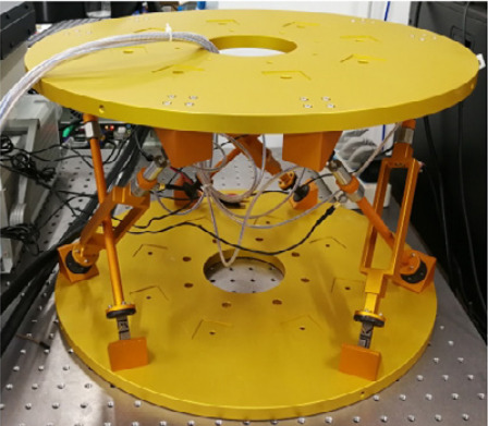
Similar to cite:yang19_dynam_model_decoup_contr_flexib (Figure ref:fig:detail_kinematics_yang19)

Example of a cubic architecture with cube's center above the top platform - Medium cube size

Large cube

Example of a cubic architecture with cube's center above the top platform - Large cube size

TODO Required size of the platforms

The minimum size of the platforms depends on the cube's size and the height between the platform and the cube's center.

Let's denote:

• $H$ the height between the cube's center and the considered platform
• $D$ the size of the cube's edges

Let's denote by $a$ and $b$ the points of both ends of one of the cube's edge.

Initially, we have:

\begin{align} a &= \frac{D}{2} \begin{bmatrix}-1 \\ -1 \\ 1\end{bmatrix} \\ b &= \frac{D}{2} \begin{bmatrix} 1 \\ -1 \\ 1\end{bmatrix} \end{align}

We rotate the cube around its center (origin of the rotated frame) such that one of its diagonal is vertical. \[ R = \begin{bmatrix} \frac{2}{\sqrt{6}} & 0 & \frac{1}{\sqrt{3}} \\ \frac{-1}{\sqrt{6}} & \frac{1}{\sqrt{2}} & \frac{1}{\sqrt{3}} \\ \frac{-1}{\sqrt{6}} & \frac{-1}{\sqrt{2}} & \frac{1}{\sqrt{3}} \end{bmatrix} \]

After rotation, the points $a$ and $b$ become:

\begin{align} a &= \frac{D}{2} \begin{bmatrix}-\frac{\sqrt{2}}{\sqrt{3}} \\ -\sqrt{2} \\ -\frac{1}{\sqrt{3}}\end{bmatrix} \\ b &= \frac{D}{2} \begin{bmatrix} \frac{\sqrt{2}}{\sqrt{3}} \\ -\sqrt{2} \\ \frac{1}{\sqrt{3}}\end{bmatrix} \end{align}

Points $a$ and $b$ define a vector $u = b - a$ that gives the orientation of one of the Stewart platform strut: \[ u = \frac{D}{\sqrt{3}} \begin{bmatrix} -\sqrt{2} \\ 0 \\ -1\end{bmatrix} \]

Then we want to find the intersection between the line that defines the strut with the plane defined by the height $H$ from the cube's center. To do so, we first find $g$ such that: \[ a_z + g u_z = -H \] We obtain:

\begin{align} g &= - \frac{H + a_z}{u_z} \\ &= \sqrt{3} \frac{H}{D} - \frac{1}{2} \end{align}

Then, the intersection point $P$ is given by:

\begin{align} P &= a + g u \\ &= \begin{bmatrix} H \sqrt{2} \\ D \frac{1}{\sqrt{2}} \\ H \end{bmatrix} \end{align}

Finally, the circle can contains the intersection point has a radius $r$:

\begin{align} r &= \sqrt{P_x^2 + P_y^2} \\ &= \sqrt{2 H^2 + \frac{1}{2}D^2} \end{align}

By symmetry, we can show that all the other intersection points will also be on the circle with a radius $r$.

For a small cube: \[ r \approx \sqrt{2} H \]

Conclusion

For each of the configuration, the Stiffness matrix is diagonal with $k_x = k_y = k_y = 2k$ with $k$ is the stiffness of each strut. However, the rotational stiffnesses are increasing with the cube's size but the required size of the platform is also increasing, so there is a trade-off here.

We found that we can have a diagonal stiffness matrix using the cubic architecture when $\{A\}$ and $\{B\}$ are located above the top platform. Depending on the cube's size, we obtain 3 different configurations.

Conclusion

Conclusion

<<sec:detail_kinematics_conclusion>>

Inertia used for experiments will be very broad => difficult to optimize the dynamics Specific geometry is not found to have a huge impact on performances. Practical implementation is important.

Geometry impacts the static and dynamical characteristics of the Stewart platform. Considering the design constrains, the slight change of geometry will not significantly impact the obtained results.

Bibliography   ignore