231 KiB
Nano Hexapod - Optimal Geometry
- Introduction
- Review of Stewart platforms
- Effect of geometry on Stewart platform properties
- The Cubic Architecture
- Nano Hexapod
- Conclusion
- Bibliography
Introduction ignore
The performance of a Stewart platform depends on its geometric configuration, especially the orientation of its struts and the positioning of its joints. During the conceptual design phase of the nano-hexapod, a preliminary geometry was selected based on general principles without detailed optimization. As the project advanced to the detailed design phase, a rigorous analysis of how geometry influences system performance became essential to ensure that the final design would meet the demanding requirements of the Nano Active Stabilization System (NASS).
In this chapter, the nano-hexapod geometry is optimized through careful analysis of how design parameters influence critical performance aspects: attainable workspace, mechanical stiffness, strut-to-strut coupling for decentralized control strategies, and dynamic response in Cartesian coordinates.
The chapter begins with a comprehensive review of existing Stewart platform designs in Section ref:sec:detail_kinematics_stewart_review, surveying various approaches to geometry, actuation, sensing, and joint design from the literature. Section ref:sec:detail_kinematics_geometry develops the analytical framework that connects geometric parameters to performance characteristics, establishing quantitative relationships that guide the optimization process. Section ref:sec:detail_kinematics_cubic examines the cubic configuration, a specific architecture that has gathered significant attention, to evaluate its suitability for the nano-hexapod application. Finally, Section ref:sec:detail_kinematics_nano_hexapod presents the optimized nano-hexapod geometry derived from these analyses and demonstrates how it addresses the specific requirements of the NASS.
Review of Stewart platforms
<<sec:detail_kinematics_stewart_review>>
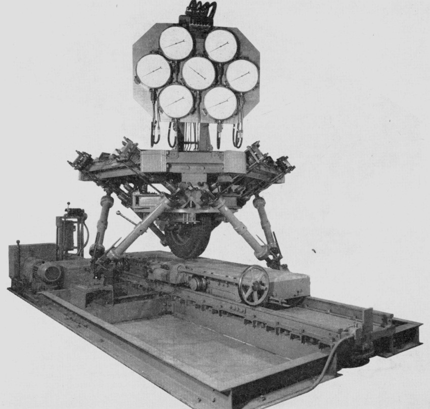
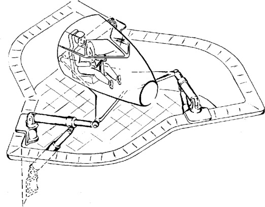
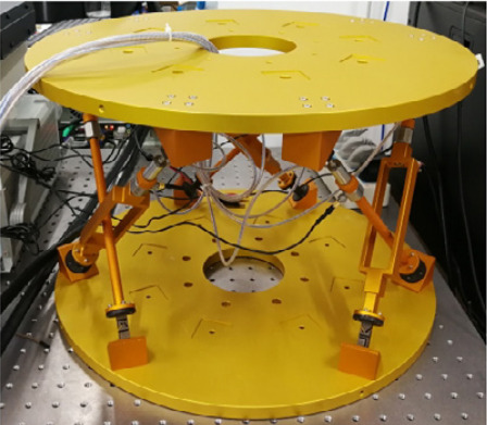
The first parallel platform similar to the Stewart platform was built in 1954 by Gough cite:&gough62_univer_tyre_test_machin, for a tyre test machine (shown in Figure ref:fig:detail_geometry_gough_paper). Subsequently, Stewart proposed a similar design for a flight simulator (shown in Figure ref:fig:detail_geometry_stewart_flight_simulator) in a 1965 publication cite:&stewart65_platf_with_six_degrees_freed. Since then, the Stewart platform (sometimes referred to as the Stewart-Gough platform) has been utilized across diverse applications cite:&dasgupta00_stewar_platf_manip, including large telescopes cite:&kazezkhan14_dynam_model_stewar_platf_nansh_radio_teles;&yun19_devel_isotr_stewar_platf_teles_secon_mirror, machine tools cite:&russo24_review_paral_kinem_machin_tools, and Synchrotron instrumentation cite:&marion04_hexap_esrf;&villar18_nanop_esrf_id16a_nano_imagin_beaml.
As explained in the conceptual phase, Stewart platforms comprise the following key elements: two plates connected by six struts, with each strut composed of a joint at each end, an actuator, and one or several sensors.
The specific geometry (i.e., position of joints and orientation of the struts) can be selected based on the application requirements, resulting in numerous designs throughout the literature. This discussion focuses primarily on Stewart platforms designed for nano-positioning and vibration control, which necessitates the use of flexible joints. The implementation of these flexible joints, will be discussed when designing the nano-hexapod flexible joints. Long stroke Stewart platforms are not addressed here as their design presents different challenges, such as singularity-free workspace and complex kinematics cite:&merlet06_paral_robot.
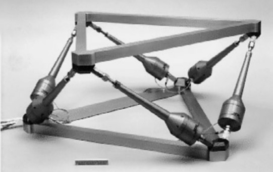
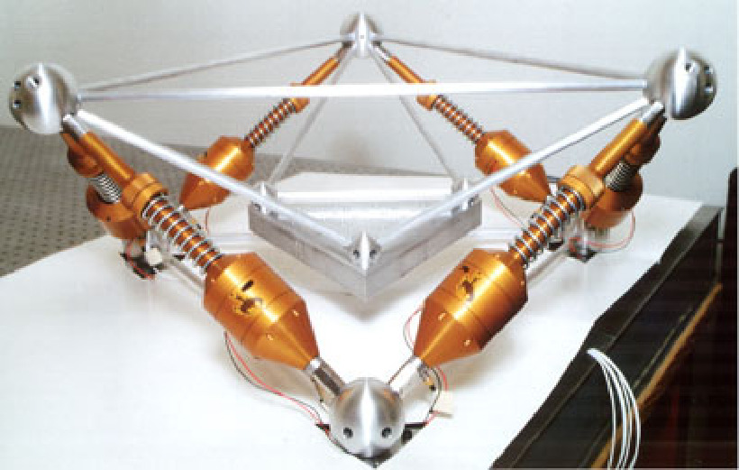
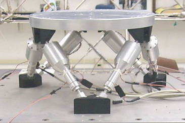
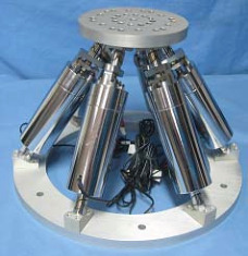
In terms of actuation, mainly two types are used: voice coil actuators and piezoelectric actuators. Voice coil actuators, providing stroke ranges from $0.5\,mm$ to $10\,mm$, are commonly implemented in cubic architectures (as illustrated in Figures ref:fig:detail_kinematics_jpl, ref:fig:detail_kinematics_uw_gsp and ref:fig:detail_kinematics_pph) and are mainly used for vibration isolation cite:&spanos95_soft_activ_vibrat_isolat;&rahman98_multiax;&thayer98_stewar;&mcinroy99_dynam;&preumont07_six_axis_singl_stage_activ. For applications requiring short stroke (typically smaller than $500\,\mu m$), piezoelectric actuators present an interesting alternative, as shown in cite:&agrawal04_algor_activ_vibrat_isolat_spacec;&furutani04_nanom_cuttin_machin_using_stewar;&yang19_dynam_model_decoup_contr_flexib. Examples of piezoelectric-actuated Stewart platforms are presented in Figures ref:fig:detail_kinematics_ulb_pz, ref:fig:detail_kinematics_uqp and ref:fig:detail_kinematics_yang19. Although less frequently encountered, magnetostrictive actuators have been successfully implemented in cite:&zhang11_six_dof (Figure ref:fig:detail_kinematics_zhang11).
\bigskip
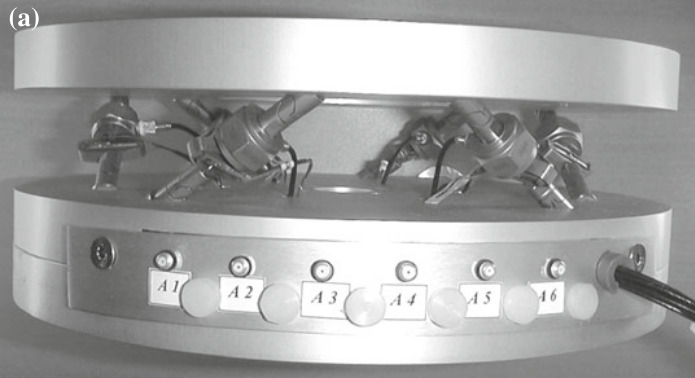
The sensors integrated in these platforms are selected based on specific control requirements, as different sensors offer distinct advantages and limitations cite:&hauge04_sensor_contr_space_based_six. Force sensors are typically integrated within the struts in a collocated arrangement with actuators to enhance control robustness. Stewart platforms incorporating force sensors are frequently utilized for vibration isolation cite:&spanos95_soft_activ_vibrat_isolat;&rahman98_multiax and active damping applications cite:&geng95_intel_contr_system_multip_degree;&abu02_stiff_soft_stewar_platf_activ, as exemplified in Figure ref:fig:detail_kinematics_ulb_pz.
Inertial sensors (accelerometers and geophones) are commonly employed in vibration isolation applications cite:&chen03_payload_point_activ_vibrat_isolat;&chi15_desig_exper_study_vcm_based. These sensors are predominantly aligned with the struts cite:&hauge04_sensor_contr_space_based_six;&li01_simul_fault_vibrat_isolat_point;&thayer02_six_axis_vibrat_isolat_system;&zhang11_six_dof;&jiao18_dynam_model_exper_analy_stewar;&tang18_decen_vibrat_contr_voice_coil, although they may also be fixed to the top platform cite:&wang16_inves_activ_vibrat_isolat_stewar.
For high-precision positioning applications, various displacement sensors are implemented, including LVDTs cite:&thayer02_six_axis_vibrat_isolat_system;&kim00_robus_track_contr_desig_dof_paral_manip;&li01_simul_fault_vibrat_isolat_point;&thayer98_stewar, capacitive sensors cite:&ting07_measur_calib_stewar_microm_system;&ting13_compos_contr_desig_stewar_nanos_platf, eddy current sensors cite:&chen03_payload_point_activ_vibrat_isolat;&furutani04_nanom_cuttin_machin_using_stewar, and strain gauges cite:&du14_piezo_actuat_high_precis_flexib. Notably, some designs incorporate external sensing methodologies rather than integrating sensors within the struts cite:&li01_simul_fault_vibrat_isolat_point;&chen03_payload_point_activ_vibrat_isolat;&ting13_compos_contr_desig_stewar_nanos_platf. A recent design cite:&naves20_desig, although not strictly speaking a Stewart platform, has demonstrated the use of 3-phase rotary motors with rotary encoders for achieving long-stroke and highly repeatable positioning, as illustrated in Figure ref:fig:detail_kinematics_naves.
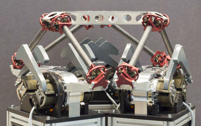
Two primary categories of Stewart platform geometry can be identified. The first is cubic architecture (examples presented in Figure ref:fig:detail_kinematics_stewart_examples_cubic), wherein struts are positioned along six sides of a cube (and therefore oriented orthogonally to each other). This architecture represents the most prevalent configuration for vibration isolation applications in the literature. Its distinctive properties will be examined in Section ref:sec:detail_kinematics_cubic. The second category comprises non-cubic architectures (Figure ref:fig:detail_kinematics_stewart_examples_non_cubic), where strut orientation and joint positioning can be optimized according to defined performance criteria. The influence of strut orientation and joint positioning on Stewart platform properties is analyzed in Section ref:sec:detail_kinematics_geometry.
\bigskip
Effect of geometry on Stewart platform properties
<<sec:detail_kinematics_geometry>>
Introduction ignore
As was demonstrated during the conceptual phase, the geometry of the Stewart platform impacts the stiffness and compliance characteristics, the mobility (or workspace), the force authority, and the dynamics of the manipulator. It is therefore essential to understand how the geometry impacts these properties, and to develop methodologies for optimizing the geometry for specific applications.
A useful analytical tool for this study is the Jacobian matrix, which depends on $\bm{b}_i$ (joints' position with respect to the top platform) and $\hat{\bm{s}}_i$ (struts' orientation). The choice of $\{A\}$ and $\{B\}$ frames, independently of the physical Stewart platform geometry, impacts the obtained kinematics and stiffness matrix, as these are defined for forces and motion evaluated at the chosen frame.
Platform Mobility / Workspace
<<ssec:detail_kinematics_geometry_mobility>>
Introduction ignore
The mobility of the Stewart platform (or any manipulator) is defined as the range of motion that it can perform. It corresponds to the set of possible poses (i.e., combined translation and rotation) of frame $\{B\}$ with respect to frame $\{A\}$. This represents a six-dimensional property which is difficult to represent. Depending on the applications, only the translation mobility (i.e., fixed orientation workspace) or the rotation mobility may be represented. This approach is equivalent to projecting the six-dimensional value into a three-dimensional space, which is easier to represent.
Mobility of parallel manipulators is inherently difficult to study as the translational and orientation workspace are coupled cite:&merlet02_still. The analysis is significantly simplified when considering small motions, as the Jacobian matrix can be used to link the strut motion to the motion of frame $\{B\}$ with respect to $\{A\}$ through eqref:eq:detail_kinematics_jacobian, which is a linear equation.
\begin{equation}\label{eq:detail_kinematics_jacobian} \begin{bmatrix} \delta l_1 \\ \delta l_2 \\ \delta l_3 \\ \delta l_4 \\ \delta l_5 \\ \delta l_6 \end{bmatrix} = \underbrace{\begin{bmatrix} {{}^A\hat{\bm{s}}_1}^T & ({}^A\bm{b}_1 \times {}^A\hat{\bm{s}}_1)^T \\ {{}^A\hat{\bm{s}}_2}^T & ({}^A\bm{b}_2 \times {}^A\hat{\bm{s}}_2)^T \\ {{}^A\hat{\bm{s}}_3}^T & ({}^A\bm{b}_3 \times {}^A\hat{\bm{s}}_3)^T \\ {{}^A\hat{\bm{s}}_4}^T & ({}^A\bm{b}_4 \times {}^A\hat{\bm{s}}_4)^T \\ {{}^A\hat{\bm{s}}_5}^T & ({}^A\bm{b}_5 \times {}^A\hat{\bm{s}}_5)^T \\ {{}^A\hat{\bm{s}}_6}^T & ({}^A\bm{b}_6 \times {}^A\hat{\bm{s}}_6)^T \end{bmatrix}}_{\bm{J}} \begin{bmatrix} \delta x \\ \delta y \\ \delta z \\ \delta \theta_x \\ \delta \theta_y \\ \delta \theta_z \end{bmatrix} = _brace{\begin{bmatrix} {{}^A\hat{\bm{s}}_1}^T & ({}^A\bm{b}_1 \times {}^A\hat{\bm{s}}_1)^T \\ {{}^A\hat{\bm{s}}_2}^T & ({}^A\bm{b}_2 \times {}^A\hat{\bm{s}}_2)^T \\ {{}^A\hat{\bm{s}}_3}^T & ({}^A\bm{b}_3 \times {}^A\hat{\bm{s}}_3)^T \\ {{}^A\hat{\bm{s}}_4}^T & ({}^A\bm{b}_4 \times {}^A\hat{\bm{s}}_4)^T \\ {{}^A\hat{\bm{s}}_5}^T & ({}^A\bm{b}_5 \times {}^A\hat{\bm{s}}_5)^T \\ {{}^A\hat{\bm{s}}_6}^T & ({}^A\bm{b}_6 \times {}^A\hat{\bm{s}}_6)^T \end{bmatrix}}_{\bm{J}} \begin{bmatrix} \delta x \\ \delta y \\ \delta z \\ \delta \theta_x \\ \delta \theta_y \\ \delta \theta_z \end{bmatrix}}_{\bm{J}} \begin{bmatrix} \delta x \\ \delta y \\ \delta z \\ \delta \theta_x \\ \delta \theta_y \\ \delta \theta_z \end{bmatrix}
\end{equation}
Therefore, the mobility of the Stewart platform (defined as the set of achievable $[\delta x\ \delta y\ \delta z\ \delta \theta_x\ \delta \theta_y\ \delta \theta_z]$) depends on two key factors: the stroke of each strut and the geometry of the Stewart platform (embodied in the Jacobian matrix). More specifically, the XYZ mobility only depends on the $\hat{\bm{s}}_i$ (orientation of struts), while the mobility in rotation also depends on $\bm{b}_i$ (position of top joints).
Mobility in translation
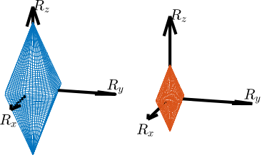
For simplicity, only translations are first considered (i.e., the Stewart platform is considered to have fixed orientation). In the general case, the translational mobility can be represented by a 3D shape having 12 faces, where each actuator limits the stroke along its axis in positive and negative directions. The faces are therefore perpendicular to the strut direction. The obtained mobility for the Stewart platform geometry shown in Figure ref:fig:detail_kinematics_mobility_trans_arch is computed and represented in Figure ref:fig:detail_kinematics_mobility_trans_result.
thetas = linspace(0, pi, 100);
phis = linspace(0, 2*pi, 100);
rs = zeros(length(thetas), length(phis));

for i = 1:length(thetas)
    for j = 1:length(phis)
        Tx = sin(thetas(i))*cos(phis(j));
        Ty = sin(thetas(i))*sin(phis(j));
        Tz = cos(thetas(i));

        dL = stewart.kinematics.J*[Tx; Ty; Tz; 0; 0; 0;]; % dL required for 1m displacement in theta/phi direction

        rs(i, j) = L_max/max(abs(dL));
    end
end

% Sphere with radius equal to actuator stroke
[Xs,Ys,Zs] = sphere;
Xs = 1e6*L_max*Xs;
Ys = 1e6*L_max*Ys;
Zs = 1e6*L_max*Zs;

[phi_grid, theta_grid] = meshgrid(phis, thetas);
X = 1e6 * rs .* sin(theta_grid) .* cos(phi_grid);
Y = 1e6 * rs .* sin(theta_grid) .* sin(phi_grid);
Z = 1e6 * rs .* cos(theta_grid);

figure('Renderer', 'painters');
hold on;
surf(X,  Y,  Z,  'FaceColor', 'none', 'LineWidth', 0.1, 'EdgeColor', [0, 0, 0]);
surf(Xs, Ys, Zs, 'FaceColor', colors(2,:), 'EdgeColor', 'none');
quiver3(0, 0, 0, 100, 0, 0, 'k', 'LineWidth', 2, 'MaxHeadSize', 0.9);
quiver3(0, 0, 0, 0, 100, 0, 'k', 'LineWidth', 2, 'MaxHeadSize', 0.9);
quiver3(0, 0, 0, 0, 0, 100, 'k', 'LineWidth', 2, 'MaxHeadSize', 0.9);
hold off;
axis equal;
grid off;
axis off;
view(55, 25);
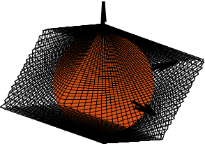
With the previous interpretations of the 12 faces making the translational mobility 3D shape, it can be concluded that for a strut stroke of $\pm d$, a sphere with radius $d$ is contained in the 3D shape and touches it in directions defined by the strut axes, as illustrated in Figure ref:fig:detail_kinematics_mobility_trans_result. This means that the mobile platform can be translated in any direction with a stroke equal to the strut stroke.
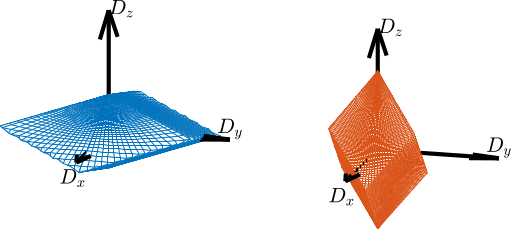
To better understand how the geometry of the Stewart platform impacts the translational mobility, two configurations are compared with struts oriented vertically (Figure ref:fig:detail_kinematics_stewart_mobility_vert_struts) and struts oriented horizontally (Figure ref:fig:detail_kinematics_stewart_mobility_hori_struts). The vertically oriented struts configuration leads to greater stroke in the horizontal direction and reduced stroke in the vertical direction (Figure ref:fig:detail_kinematics_mobility_translation_strut_orientation). Conversely, horizontal oriented struts configuration provides more stroke in the vertical direction.
It may seem counterintuitive that less stroke is available in the direction of the struts. This phenomenon occurs because the struts form a lever mechanism that amplifies the motion. The amplification factor increases when the struts have a high angle with the direction of motion and equals one (i.e. is minimal) when aligned with the direction of motion.


Mobility in rotation
As shown by equation eqref:eq:detail_kinematics_jacobian, the rotational mobility depends both on the orientation of the struts and on the location of the top joints. Similarly to the translational case, to increase the rotational mobility in one direction, it is advantageous to have the struts more perpendicular to the rotational direction.
For instance, having the struts more vertical (Figure ref:fig:detail_kinematics_stewart_mobility_vert_struts) provides less rotational stroke along the vertical direction than having the struts oriented more horizontally (Figure ref:fig:detail_kinematics_stewart_mobility_hori_struts).
Two cases are considered with the same strut orientation but with different top joint positions: struts positioned close to each other (Figure ref:fig:detail_kinematics_stewart_mobility_close_struts) and struts positioned further apart (Figure ref:fig:detail_kinematics_stewart_mobility_space_struts). The mobility for pure rotations is compared in Figure ref:fig:detail_kinematics_mobility_angle_strut_distance. Having struts further apart decreases the "lever arm" and therefore reduces the rotational mobility.


Combined translations and rotations
It is possible to consider combined translations and rotations, although displaying such mobility becomes more complex. For a fixed geometry and a desired mobility (combined translations and rotations), it is possible to estimate the required minimum actuator stroke. This analysis is conducted in Section ref:sec:detail_kinematics_nano_hexapod to estimate the required actuator stroke for the nano-hexapod geometry.
Stiffness
<<ssec:detail_kinematics_geometry_stiffness>>
Introduction ignore
The stiffness matrix defines how the top platform of the Stewart platform (i.e. frame $\{B\}$) deforms with respect to its fixed base (i.e. frame $\{A\}$) due to static forces/torques applied between frames $\{A\}$ and $\{B\}$. It depends on the Jacobian matrix (i.e., the geometry) and the strut axial stiffness as shown in equation eqref:eq:detail_kinematics_stiffness_matrix. The contribution of joints stiffness is not considered here, as the joints were optimized after the geometry was fixed. However, theoretical frameworks for evaluating flexible joint contribution to the stiffness matrix have been established in the literature cite:&mcinroy00_desig_contr_flexur_joint_hexap;&mcinroy02_model_desig_flexur_joint_stewar.
\begin{equation}\label{eq:detail_kinematics_stiffness_matrix} \bm{K} = \bm{J}^T \bm{\mathcal{K}} \bm{J}
\end{equation}
It is assumed that the stiffness of all struts is the same: $\bm{\mathcal{K}} = k \cdot \mathbf{I}_6$. In that case, the obtained stiffness matrix linearly depends on the strut stiffness $k$, and is structured as shown in equation eqref:eq:detail_kinematics_stiffness_matrix_simplified.
\begin{equation}\label{eq:detail_kinematics_stiffness_matrix_simplified}
\bm{K} = k \bm{J}^T \bm{J} =
k ≤ft[
\begin{array}{c|c}
Σi = 06 \hat{\bm{s}}_i ⋅ \hat{\bm{s}}_i^T & Σi = 06 \bm{\hat{s}}_i ⋅ ({}^A\bm{b}_i × {}^A\hat{\bm{s}}_i)^T
\hline
Σi = 06 ({}^A\bm{b}_i × {}^A\hat{\bm{s}}_i) ⋅ \hat{\bm{s}}_i^T & Σi = 06 ({}^A\bm{b}_i × {}^A\hat{\bm{s}}_i) ⋅ ({}^A\bm{b}_i × {}^A\hat{\bm{s}}_i)^T\\
\end{array} \right]
\end{equation}
Translation Stiffness
As shown by equation eqref:eq:detail_kinematics_stiffness_matrix_simplified, the translation stiffnesses (the $3 \times 3$ top left terms of the stiffness matrix) only depend on the orientation of the struts and not their location: $\hat{\bm{s}}_i \cdot \hat{\bm{s}}_i^T$. In the extreme case where all struts are vertical ($s_i = [0\ 0\ 1]$), a vertical stiffness of $6k$ is achieved, but with null stiffness in the horizontal directions. If two struts are aligned with the X axis, two struts with the Y axis, and two struts with the Z axis, then $\hat{\bm{s}}_i \cdot \hat{\bm{s}}_i^T = 2 \bm{I}_3$, resulting in well-distributed stiffness along all directions. This configuration corresponds to the cubic architecture presented in Section ref:sec:detail_kinematics_cubic.
When the struts are oriented more vertically, as shown in Figure ref:fig:detail_kinematics_stewart_mobility_vert_struts, the vertical stiffness increases while the horizontal stiffness decreases. Additionally, $R_x$ and $R_y$ stiffness increases while $R_z$ stiffness decreases. The opposite conclusions apply if struts are oriented more horizontally, illustrated in Figure ref:fig:detail_kinematics_stewart_mobility_hori_struts.
Rotational Stiffness
The rotational stiffnesses depend both on the orientation of the struts and on the location of the top joints with respect to the considered center of rotation (i.e., the location of frame $\{A\}$). With the same orientation but increased distances to the frame $\{A\}$ by a factor of 2, the rotational stiffness is increased by a factor of 4. Therefore, the compact Stewart platform depicted in Figure ref:fig:detail_kinematics_stewart_mobility_close_struts has less rotational stiffness than the Stewart platform shown in Figure ref:fig:detail_kinematics_stewart_mobility_space_struts.
Diagonal Stiffness Matrix
Having a diagonal stiffness matrix $\bm{K}$ can be beneficial for control purposes as it would make the plant in the Cartesian frame decoupled at low frequency. This property depends on both the geometry and the chosen $\{A\}$ frame. For specific geometry and choice of $\{A\}$ frame, it is possible to achieve a diagonal $K$ matrix. This is discussed in Section ref:ssec:detail_kinematics_cubic_static.
Dynamical properties
<<ssec:detail_kinematics_geometry_dynamics>>
The dynamical equations (both in the Cartesian frame and in the frame of the struts) for the Stewart platform were derived during the conceptual phase with simplifying assumptions (massless struts and perfect joints). The dynamics depends both on the geometry (Jacobian matrix) and on the payload being placed on top of the platform.
Under very specific conditions, the equations of motion in the Cartesian frame, given by equation eqref:eq:detail_kinematics_transfer_function_cart, can be decoupled. These conditions are studied in Section ref:ssec:detail_kinematics_cubic_dynamic.
\begin{equation}\label{eq:detail_kinematics_transfer_function_cart} \frac{{\mathcal{X}}}{\bm{\mathcal{F}}}(s) = ( \bm{M} s^2 + \bm{J}T \bm{\mathcal{C}} \bm{J} s + \bm{J}T \bm{\mathcal{K}} \bm{J} )-1
\end{equation}
In the frame of the struts, the equations of motion eqref:eq:detail_kinematics_transfer_function_struts are well decoupled at low frequency. This is why most Stewart platforms are controlled in the frame of the struts: below the resonance frequency, the system is well decoupled and SISO control may be applied for each strut, independently of the payload being used.
\begin{equation}\label{eq:detail_kinematics_transfer_function_struts} \frac{\bm{\mathcal{L}}}{\bm{f}}(s) = ( \bm{J}-T \bm{M} \bm{J}-1 s^2 + \bm{\mathcal{C}} + \bm{\mathcal{K}} )-1
\end{equation}
Coupling between sensors (force sensors, relative position sensors or inertial sensors) in different struts may also be important for decentralized control. In section ref:ssec:detail_kinematics_decentralized_control, it will be studied whether the Stewart platform geometry can be optimized to have lower coupling between the struts.
Conclusion
The effects of two changes in the manipulator's geometry, namely the position and orientation of the struts, are summarized in Table ref:tab:detail_kinematics_geometry. These results could have been easily deduced based on mechanical principles, but thanks to the kinematic analysis, they can be quantified. These trade-offs provide important guidelines when choosing the Stewart platform geometry.
| Struts | Vertically Oriented | Increased separation |
|---|---|---|
| Vertical stiffness | $\nearrow$ | $=$ |
| Horizontal stiffness | $\searrow$ | $=$ |
| Vertical rotation stiffness | $\searrow$ | $\nearrow$ |
| Horizontal rotation stiffness | $\nearrow$ | $\nearrow$ |
| Vertical mobility | $\searrow$ | $=$ |
| Horizontal mobility | $\nearrow$ | $=$ |
| Vertical rotation mobility | $\nearrow$ | $\searrow$ |
| Horizontal rotation mobility | $\searrow$ | $\searrow$ |
The Cubic Architecture
<<sec:detail_kinematics_cubic>>
Introduction ignore
The Cubic configuration for the Stewart platform was first proposed by Dr. Gough in a comment to the original paper by Dr. Stewart cite:&stewart65_platf_with_six_degrees_freed. This configuration is characterized by active struts arranged in a mutually orthogonal configuration connecting the corners of a cube, as shown in Figure ref:fig:detail_kinematics_cubic_architecture_example.
Typically, the struts have similar length to the cube's edges, as illustrated in Figure ref:fig:detail_kinematics_cubic_architecture_example. Practical implementations of such configurations can be observed in Figures ref:fig:detail_kinematics_jpl, ref:fig:detail_kinematics_uw_gsp and ref:fig:detail_kinematics_uqp. It is also possible to implement designs with strut lengths smaller than the cube's edges (Figure ref:fig:detail_kinematics_cubic_architecture_example_small), as exemplified in Figure ref:fig:detail_kinematics_ulb_pz.
Several advantageous properties attributed to the cubic configuration have contributed to its widespread adoption cite:&geng94_six_degree_of_freed_activ;&preumont07_six_axis_singl_stage_activ;&jafari03_orthog_gough_stewar_platf_microm: simplified kinematics relationships and dynamical analysis cite:&geng94_six_degree_of_freed_activ; uniform stiffness in all directions cite:&hanieh03_activ_stewar; uniform mobility cite:&preumont18_vibrat_contr_activ_struc_fourt_edition, chapt.8.5.2; and minimization of the cross coupling between actuators and sensors in different struts cite:&preumont07_six_axis_singl_stage_activ. This minimization is attributed to the fact that the struts are orthogonal to each other, and is said to facilitate collocated sensor-actuator control system design, i.e., the implementation of decentralized control cite:&geng94_six_degree_of_freed_activ;&thayer02_six_axis_vibrat_isolat_system.
These properties are examined in this section to assess their relevance for the nano-hexapod. The mobility and stiffness properties of the cubic configuration are analyzed in Section ref:ssec:detail_kinematics_cubic_static. Dynamical decoupling is investigated in Section ref:ssec:detail_kinematics_cubic_dynamic, while decentralized control, crucial for the NASS, is examined in Section ref:ssec:detail_kinematics_decentralized_control. Given that the cubic architecture imposes strict geometric constraints, alternative designs are proposed in Section ref:ssec:detail_kinematics_cubic_design. The ultimate objective is to determine the suitability of the cubic architecture for the nano-hexapod.
Static Properties
<<ssec:detail_kinematics_cubic_static>>
Stiffness matrix for the Cubic architecture
Consider the cubic architecture shown in Figure ref:fig:detail_kinematics_cubic_schematic_full. The unit vectors corresponding to the edges of the cube are described by equation eqref:eq:detail_kinematics_cubic_s.
\begin{equation}\label{eq:detail_kinematics_cubic_s} \hat{\bm{s}}_1 = \begin{bmatrix} \frac{\sqrt{2}}{\sqrt{3}} \\ 0 \\ \frac{1}{\sqrt{3}} \end{bmatrix} \quad \hat{\bm{s}}_2 = \begin{bmatrix} \frac{-1}{\sqrt{6}} \\ \frac{-1}{\sqrt{2}} \\ \frac{1}{\sqrt{3}} \end{bmatrix} \quad \hat{\bm{s}}_3 = \begin{bmatrix} \frac{-1}{\sqrt{6}} \\ \frac{ 1}{\sqrt{2}} \\ \frac{1}{\sqrt{3}} \end{bmatrix} \quad \hat{\bm{s}}_4 = \begin{bmatrix} \frac{\sqrt{2}}{\sqrt{3}} \\ 0 \\ \frac{1}{\sqrt{3}} \end{bmatrix} \quad \hat{\bm{s}}_5 = \begin{bmatrix} \frac{-1}{\sqrt{6}} \\ \frac{-1}{\sqrt{2}} \\ \frac{1}{\sqrt{3}} \end{bmatrix} \quad \hat{\bm{s}}_6 = \begin{bmatrix} \frac{-1}{\sqrt{6}} \\ \frac{ 1}{\sqrt{2}} \\ \frac{1}{\sqrt{3}} \end{bmatrix} \quad \hat{\bm{s}}_2 = \begin{bmatrix} \frac{-1}{\sqrt{6}} \\ \frac{-1}{\sqrt{2}} \\ \frac{1}{\sqrt{3}} \end{bmatrix} \quad \hat{\bm{s}}_3 = \begin{bmatrix} \frac{-1}{\sqrt{6}} \\ \frac{ 1}{\sqrt{2}} \\ \frac{1}{\sqrt{3}} \end{bmatrix} \quad \hat{\bm{s}}_4 = \begin{bmatrix} \frac{\sqrt{2}}{\sqrt{3}} \\ 0 \\ \frac{1}{\sqrt{3}} \end{bmatrix} \quad \hat{\bm{s}}_5 = \begin{bmatrix} \frac{-1}{\sqrt{6}} \\ \frac{-1}{\sqrt{2}} \\ \frac{1}{\sqrt{3}} \end{bmatrix} \quad \hat{\bm{s}}_6 = \begin{bmatrix} \frac{-1}{\sqrt{6}} \\ \frac{ 1}{\sqrt{2}} \\ \frac{1}{\sqrt{3}} \end{bmatrix} \quad \hat{\bm{s}}_3 = \begin{bmatrix} \frac{-1}{\sqrt{6}} \\ \frac{ 1}{\sqrt{2}} \\ \frac{1}{\sqrt{3}} \end{bmatrix} \quad \hat{\bm{s}}_4 = \begin{bmatrix} \frac{\sqrt{2}}{\sqrt{3}} \\ 0 \\ \frac{1}{\sqrt{3}} \end{bmatrix} \quad \hat{\bm{s}}_5 = \begin{bmatrix} \frac{-1}{\sqrt{6}} \\ \frac{-1}{\sqrt{2}} \\ \frac{1}{\sqrt{3}} \end{bmatrix} \quad \hat{\bm{s}}_6 = \begin{bmatrix} \frac{-1}{\sqrt{6}} \\ \frac{ 1}{\sqrt{2}} \\ \frac{1}{\sqrt{3}} \end{bmatrix} \quad \hat{\bm{s}}_4 = \begin{bmatrix} \frac{\sqrt{2}}{\sqrt{3}} \\ 0 \\ \frac{1}{\sqrt{3}} \end{bmatrix} \quad \hat{\bm{s}}_5 = \begin{bmatrix} \frac{-1}{\sqrt{6}} \\ \frac{-1}{\sqrt{2}} \\ \frac{1}{\sqrt{3}} \end{bmatrix} \quad \hat{\bm{s}}_6 = \begin{bmatrix} \frac{-1}{\sqrt{6}} \\ \frac{ 1}{\sqrt{2}} \\ \frac{1}{\sqrt{3}} \end{bmatrix} \quad \hat{\bm{s}}_5 = \begin{bmatrix} \frac{-1}{\sqrt{6}} \\ \frac{-1}{\sqrt{2}} \\ \frac{1}{\sqrt{3}} \end{bmatrix} \quad \hat{\bm{s}}_6 = \begin{bmatrix} \frac{-1}{\sqrt{6}} \\ \frac{ 1}{\sqrt{2}} \\ \frac{1}{\sqrt{3}} \end{bmatrix} \quad \hat{\bm{s}}_6 = \begin{bmatrix} \frac{-1}{\sqrt{6}} \\ \frac{ 1}{\sqrt{2}} \\ \frac{1}{\sqrt{3}} \end{bmatrix}
\end{equation}
  \begin{tikzpicture}
    \begin{scope}[rotate={45}, shift={(0, 0, -4)}]
      % We first define the coordinate of the points of the Cube
      \coordinate[] (bot) at (0,0,4);
      \coordinate[] (top) at (4,4,0);
      \coordinate[] (A1) at (0,0,0);
      \coordinate[] (A2) at (4,0,4);
      \coordinate[] (A3) at (0,4,4);
      \coordinate[] (B1) at (4,0,0);
      \coordinate[] (B2) at (4,4,4);
      \coordinate[] (B3) at (0,4,0);

      % Center of the Cube
      \coordinate[] (cubecenter) at ($0.5*(bot) + 0.5*(top)$);

      % We draw parts of the cube that corresponds to the Stewart platform
      \draw[] (A1)node[]{$\bullet$} -- (B1)node[]{$\bullet$} -- (A2)node[]{$\bullet$} -- (B2)node[]{$\bullet$} -- (A3)node[]{$\bullet$} -- (B3)node[]{$\bullet$} -- (A1);

      % ai and bi are computed
      \def\lfrom{0.0}
      \def\lto{1.0}

      \coordinate(a1) at ($(A1) - \lfrom*(A1) + \lfrom*(B1)$);
      \coordinate(b1) at ($(A1) - \lto*(A1)   + \lto*(B1)$);
      \coordinate(a2) at ($(A2) - \lfrom*(A2) + \lfrom*(B1)$);
      \coordinate(b2) at ($(A2) - \lto*(A2)   + \lto*(B1)$);
      \coordinate(a3) at ($(A2) - \lfrom*(A2) + \lfrom*(B2)$);
      \coordinate(b3) at ($(A2) - \lto*(A2)   + \lto*(B2)$);
      \coordinate(a4) at ($(A3) - \lfrom*(A3) + \lfrom*(B2)$);
      \coordinate(b4) at ($(A3) - \lto*(A3)   + \lto*(B2)$);
      \coordinate(a5) at ($(A3) - \lfrom*(A3) + \lfrom*(B3)$);
      \coordinate(b5) at ($(A3) - \lto*(A3)   + \lto*(B3)$);
      \coordinate(a6) at ($(A1) - \lfrom*(A1) + \lfrom*(B3)$);
      \coordinate(b6) at ($(A1) - \lto*(A1)   + \lto*(B3)$);

      % We draw the fixed and mobiles platforms
      \path[fill=colorblue, opacity=0.2] (a1) -- (a2) -- (a3) -- (a4) -- (a5) -- (a6) -- cycle;
      \path[fill=colorblue, opacity=0.2] (b1) -- (b2) -- (b3) -- (b4) -- (b5) -- (b6) -- cycle;
      \draw[color=colorblue, dashed] (a1) -- (a2) -- (a3) -- (a4) -- (a5) -- (a6) -- cycle;
      \draw[color=colorblue, dashed] (b1) -- (b2) -- (b3) -- (b4) -- (b5) -- (b6) -- cycle;

      % The legs of the hexapod are drawn
      \draw[color=colorblue] (a1)node{$\bullet$} -- (b1)node{$\bullet$};
      \draw[color=colorblue] (a2)node{$\bullet$} -- (b2)node{$\bullet$};
      \draw[color=colorblue] (a3)node{$\bullet$} -- (b3)node{$\bullet$};
      \draw[color=colorblue] (a4)node{$\bullet$} -- (b4)node{$\bullet$};
      \draw[color=colorblue] (a5)node{$\bullet$} -- (b5)node{$\bullet$};
      \draw[color=colorblue] (a6)node{$\bullet$} -- (b6)node{$\bullet$};

      % Unit vector
      \draw[color=colorred, ->] ($0.9*(a1)+0.1*(b1)$)node{$\bullet$} -- ($0.65*(a1)+0.35*(b1)$)node[right]{$\hat{\bm{s}}_3$};
      \draw[color=colorred, ->] ($0.9*(a2)+0.1*(b2)$)node{$\bullet$} -- ($0.65*(a2)+0.35*(b2)$)node[left]{$\hat{\bm{s}}_4$};
      \draw[color=colorred, ->] ($0.9*(a3)+0.1*(b3)$)node{$\bullet$} -- ($0.65*(a3)+0.35*(b3)$)node[below]{$\hat{\bm{s}}_5$};
      \draw[color=colorred, ->] ($0.9*(a4)+0.1*(b4)$)node{$\bullet$} -- ($0.65*(a4)+0.35*(b4)$)node[below]{$\hat{\bm{s}}_6$};
      \draw[color=colorred, ->] ($0.9*(a5)+0.1*(b5)$)node{$\bullet$} -- ($0.65*(a5)+0.35*(b5)$)node[left]{$\hat{\bm{s}}_1$};
      \draw[color=colorred, ->] ($0.9*(a6)+0.1*(b6)$)node{$\bullet$} -- ($0.65*(a6)+0.35*(b6)$)node[right]{$\hat{\bm{s}}_2$};

      % Labels
      \node[above=0.1 of B1] {$\tilde{\bm{b}}_3 = \tilde{\bm{b}}_4$};
      \node[above=0.1 of B2] {$\tilde{\bm{b}}_5 = \tilde{\bm{b}}_6$};
      \node[above=0.1 of B3] {$\tilde{\bm{b}}_1 = \tilde{\bm{b}}_2$};
    \end{scope}

    % Height of the Hexapod
    \coordinate[] (sizepos) at ($(a2)+(0.2, 0)$);
    \coordinate[] (origin) at (0,0,0);

    \draw[->, color=colorgreen] (cubecenter.center) node[above right]{$\{B\}$} -- ++(0,0,1);
    \draw[->, color=colorgreen] (cubecenter.center) -- ++(1,0,0);
    \draw[->, color=colorgreen] (cubecenter.center) -- ++(0,1,0);

    \node[] at (cubecenter.center){$\bullet$};
    \node[above left] at (cubecenter.center){$\{C\}$};

    % Useful part of the cube
    \draw[<->, dashed] ($(A2)+(0.5,0)$) -- node[midway, right]{$H_{C}$} ($(B1)+(0.5,0)$);
\end{tikzpicture} \begin{tikzpicture}
\begin{scope}[rotate={45}, shift={(0, 0, -4)}]
% We first define the coordinate of the points of the Cube
\coordinate[] (bot) at (0,0,4);
\coordinate[] (top) at (4,4,0);
\coordinate[] (A1) at (0,0,0);
\coordinate[] (A2) at (4,0,4);
\coordinate[] (A3) at (0,4,4);
\coordinate[] (B1) at (4,0,0);
\coordinate[] (B2) at (4,4,4);
\coordinate[] (B3) at (0,4,0);
% Center of the Cube
\coordinate[] (cubecenter) at ($0.5*(bot) + 0.5*(top)$);
% We draw parts of the cube that corresponds to the Stewart platform
\draw[] (A1)node[]{$\bullet$} -- (B1)node[]{$\bullet$} -- (A2)node[]{$\bullet$} -- (B2)node[]{$\bullet$} -- (A3)node[]{$\bullet$} -- (B3)node[]{$\bullet$} -- (A1);
% ai and bi are computed
\def\lfrom{0.2}
\def\lto{0.8}
\coordinate(a1) at ($(A1) - \lfrom*(A1) + \lfrom*(B1)$);
\coordinate(b1) at ($(A1) - \lto*(A1) + \lto*(B1)$);
\coordinate(a2) at ($(A2) - \lfrom*(A2) + \lfrom*(B1)$);
\coordinate(b2) at ($(A2) - \lto*(A2) + \lto*(B1)$);
\coordinate(a3) at ($(A2) - \lfrom*(A2) + \lfrom*(B2)$);
\coordinate(b3) at ($(A2) - \lto*(A2) + \lto*(B2)$);
\coordinate(a4) at ($(A3) - \lfrom*(A3) + \lfrom*(B2)$);
\coordinate(b4) at ($(A3) - \lto*(A3) + \lto*(B2)$);
\coordinate(a5) at ($(A3) - \lfrom*(A3) + \lfrom*(B3)$);
\coordinate(b5) at ($(A3) - \lto*(A3) + \lto*(B3)$);
\coordinate(a6) at ($(A1) - \lfrom*(A1) + \lfrom*(B3)$);
\coordinate(b6) at ($(A1) - \lto*(A1) + \lto*(B3)$);
% We draw the fixed and mobiles platforms
\path[fill=colorblue, opacity=0.2] (a1) -- (a2) -- (a3) -- (a4) -- (a5) -- (a6) -- cycle;
\path[fill=colorblue, opacity=0.2] (b1) -- (b2) -- (b3) -- (b4) -- (b5) -- (b6) -- cycle;
\draw[color=colorblue, dashed] (a1) -- (a2) -- (a3) -- (a4) -- (a5) -- (a6) -- cycle;
\draw[color=colorblue, dashed] (b1) -- (b2) -- (b3) -- (b4) -- (b5) -- (b6) -- cycle;
% The legs of the hexapod are drawn
\draw[color=colorblue] (a1)node{$\bullet$} -- (b1)node{$\bullet$}node[below right]{$\bm{b}_3$};
\draw[color=colorblue] (a2)node{$\bullet$} -- (b2)node{$\bullet$}node[right]{$\bm{b}_4$};
\draw[color=colorblue] (a3)node{$\bullet$} -- (b3)node{$\bullet$}node[above right]{$\bm{b}_5$};
\draw[color=colorblue] (a4)node{$\bullet$} -- (b4)node{$\bullet$}node[above left]{$\bm{b}_6$};
\draw[color=colorblue] (a5)node{$\bullet$} -- (b5)node{$\bullet$}node[left]{$\bm{b}_1$};
\draw[color=colorblue] (a6)node{$\bullet$} -- (b6)node{$\bullet$}node[below left]{$\bm{b}_2$};
\end{scope}
% Height of the Hexapod
\coordinate[] (sizepos) at ($(a2)+(0.2, 0)$);
\coordinate[] (origin) at (0,0,0);
\draw[->, color=colorgreen] ($(cubecenter.center)+(0,2.0,0)$) node[above right]{$\{B\}$} -- ++(0,0,1);
\draw[->, color=colorgreen] ($(cubecenter.center)+(0,2.0,0)$) -- ++(1,0,0);
\draw[->, color=colorgreen] ($(cubecenter.center)+(0,2.0,0)$) -- ++(0,1,0);
\node[] at (cubecenter.center){$\bullet$};
\node[right] at (cubecenter.center){$\{C\}$};
\draw[<->, dashed] (cubecenter.center) -- node[midway, right]{$H$} ($(cubecenter.center)+(0,2.0,0)$);
\end{tikzpicture}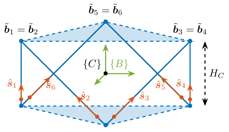
Coordinates of the cube's vertices relevant for the top joints, expressed with respect to the cube's center, are shown in equation eqref:eq:detail_kinematics_cubic_vertices.
\begin{equation}\label{eq:detail_kinematics_cubic_vertices} ~{\bm{b}}_1 = ~{\bm{b}}_2 = H_c \begin{bmatrix} \frac{1}{\sqrt{2}} \\ \frac{-\sqrt{3}}{\sqrt{2}} \\ \frac{1}{2} \end{bmatrix}, \quad \tilde{\bm{b}}_3 = \tilde{\bm{b}}_4 = H_c \begin{bmatrix} \frac{1}{\sqrt{2}} \\ \frac{ \sqrt{3}}{\sqrt{2}} \\ \frac{1}{2} \end{bmatrix}, \quad \tilde{\bm{b}}_5 = \tilde{\bm{b}}_6 = H_c \begin{bmatrix} \frac{-2}{\sqrt{2}} \\ 0 \\ \frac{1}{2} \end{bmatrix}, \quad ~{\bm{b}}_3 = ~{\bm{b}}_4 = H_c \begin{bmatrix} \frac{1}{\sqrt{2}} \\ \frac{ \sqrt{3}}{\sqrt{2}} \\ \frac{1}{2} \end{bmatrix}, \quad \tilde{\bm{b}}_5 = \tilde{\bm{b}}_6 = H_c \begin{bmatrix} \frac{-2}{\sqrt{2}} \\ 0 \\ \frac{1}{2} \end{bmatrix}, \quad ~{\bm{b}}_5 = ~{\bm{b}}_6 = H_c \begin{bmatrix} \frac{-2}{\sqrt{2}} \\ 0 \\ \frac{1}{2} \end{bmatrix}
\end{equation}
In the case where top joints are positioned at the cube's vertices, a diagonal stiffness matrix is obtained as shown in equation eqref:eq:detail_kinematics_cubic_stiffness. Translation stiffness is twice the stiffness of the struts, and rotational stiffness is proportional to the square of the cube's size $H_c$.
\begin{equation}\label{eq:detail_kinematics_cubic_stiffness}
\bm{K}_{\{B\} = \{C\}} = k \begin{bmatrix}
2 & 0 & 0 & 0 & 0 & 0
0 & 2 & 0 & 0 & 0 & 0
0 & 0 & 2 & 0 & 0 & 0
0 & 0 & 0 & \frac{3}{2} H_c^2 & 0 & 0
0 & 0 & 0 & 0 & \frac{3}{2} H_c^2 & 0
0 & 0 & 0 & 0 & 0 & 6 H_c^2 \\
\end{bmatrix}
\end{equation}
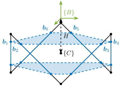
However, typically, the top joints are not placed at the cube's vertices but at positions along the cube's edges (Figure ref:fig:detail_kinematics_cubic_schematic). In that case, the location of the top joints can be expressed by equation eqref:eq:detail_kinematics_cubic_edges, yet the computed stiffness matrix remains identical to Equation eqref:eq:detail_kinematics_cubic_stiffness.
\begin{equation}\label{eq:detail_kinematics_cubic_edges} \bm{b}_i = ~{\bm{b}}_i + α \hat{\bm{s}}_i
\end{equation}
The stiffness matrix is therefore diagonal when the considered $\{B\}$ frame is located at the center of the cube (shown by frame $\{C\}$). This means that static forces (resp torques) applied at the cube's center will induce pure translations (resp rotations around the cube's center). This specific location where the stiffness matrix is diagonal is referred to as the "Center of Stiffness" (analogous to the "Center of Mass" where the mass matrix is diagonal).
%% Analytical formula for Stiffness matrix of the Cubic Stewart platform
% Define symbolic variables
syms k Hc alpha H

assume(k > 0); % k is positive real
assume(Hc, 'real'); % Hc is real
assume(H, 'real'); % H is real
assume(alpha, 'real'); % alpha is real

% Define si matrix (edges of the cubes)
si = 1/sqrt(3)*[
  [ sqrt(2),    0,        1]; ...
  [-sqrt(2)/2, -sqrt(3/2), 1]; ...
  [-sqrt(2)/2,  sqrt(3/2), 1]; ...
  [ sqrt(2),    0,        1]; ...
  [-sqrt(2)/2, -sqrt(3/2), 1]; ...
  [-sqrt(2)/2,  sqrt(3/2), 1]  ...
];

% Define ci matrix (vertices of the cubes)
ci = Hc * [
  [1/sqrt(2), -sqrt(3)/sqrt(2), 0.5]; ...
  [1/sqrt(2), -sqrt(3)/sqrt(2), 0.5]; ...
  [1/sqrt(2),  sqrt(3)/sqrt(2), 0.5]; ...
  [1/sqrt(2),  sqrt(3)/sqrt(2), 0.5]; ...
  [-sqrt(2),   0,               0.5]; ...
  [-sqrt(2),   0,               0.5]  ...
];

% Apply vertical shift to ci
ci = ci + H * [0, 0, 1];

% Calculate bi vectors (Stewart platform top joints)
bi = ci + alpha * si;

% Initialize stiffness matrix
K = sym(zeros(6,6));

% Calculate elements of the stiffness matrix
for i = 1:6
    % Extract vectors for each leg
    s_i = si(i,:)';
    b_i = bi(i,:)';

    % Calculate cross product vector
    cross_bs = cross(b_i, s_i);

    % Build matrix blocks
    K(1:3, 4:6) = K(1:3, 4:6) + s_i * cross_bs';
    K(4:6, 1:3) = K(4:6, 1:3) + cross_bs * s_i';
    K(1:3, 1:3) = K(1:3, 1:3) + s_i * s_i';
    K(4:6, 4:6) = K(4:6, 4:6) + cross_bs * cross_bs';
end

% Scale by stiffness coefficient
K = k * K;

% Simplify the expressions
K = simplify(K);

% Display the analytical stiffness matrix
disp('Analytical Stiffness Matrix:');
pretty(K);
Effect of having frame $\{B\}$ off-centered
When the reference frames $\{A\}$ and $\{B\}$ are shifted from the cube's center, off-diagonal elements emerge in the stiffness matrix.
Considering a vertical shift as shown in Figure ref:fig:detail_kinematics_cubic_schematic, the stiffness matrix transforms into that shown in Equation eqref:eq:detail_kinematics_cubic_stiffness_off_centered. Off-diagonal elements increase proportionally with the height difference between the cube's center and the considered $\{B\}$ frame.
\begin{equation}\label{eq:detail_kinematics_cubic_stiffness_off_centered}
\bm{K}_{\{B\} ≠ \{C\}} = k \begin{bmatrix}
2 & 0 & 0 & 0 & -2 H & 0
0 & 2 & 0 & 2 H & 0 & 0
0 & 0 & 2 & 0 & 0 & 0
0 & 2 H & 0 & \frac{3}{2} H_c^2 + 2 H^2 & 0 & 0
-2 H & 0 & 0 & 0 & \frac{3}{2} H_c^2 + 2 H^2 & 0
0 & 0 & 0 & 0 & 0 & 6 H_c^2 \\
\end{bmatrix}
\end{equation}
This stiffness matrix structure is characteristic of Stewart platforms exhibiting symmetry, and is not an exclusive property of cubic architectures. Therefore, the stiffness characteristics of the cubic architecture are only distinctive when considering a reference frame located at the cube's center. This poses a practical limitation, as in most applications, the relevant frame (where motion is of interest and forces are applied) is located above the top platform.
It should be noted that for the stiffness matrix to be diagonal, the cube's center doesn't need to coincide with the geometric center of the Stewart platform. This observation leads to the interesting alternative architectures presented in Section ref:ssec:detail_kinematics_cubic_design.
Uniform Mobility
The translational mobility of the Stewart platform with constant orientation was analyzed. Considering limited actuator stroke (elongation of each strut), the maximum achievable positions in XYZ space were estimated. The resulting mobility in X, Y, and Z directions for the cubic architecture is illustrated in Figure ref:fig:detail_kinematics_cubic_mobility_translations.
The translational workspace analysis reveals that for the cubic architecture, the achievable positions form a cube whose axes align with the struts, with the cube's edge length corresponding to the strut axial stroke. These findings suggest that the mobility pattern is more subtle than sometimes described in the literature cite:&mcinroy00_desig_contr_flexur_joint_hexap, exhibiting uniformity primarily along directions aligned with the cube's edges rather than uniform spherical distribution in all XYZ directions. This configuration still offers more consistent mobility characteristics compared to alternative architectures illustrated in Figure ref:fig:detail_kinematics_mobility_trans.
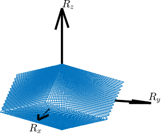
The rotational mobility, illustrated in Figure ref:fig:detail_kinematics_cubic_mobility_rotations, exhibits greater achievable angular stroke in the $R_x$ and $R_y$ directions compared to the $R_z$ direction. Furthermore, an inverse relationship exists between the cube's dimension and rotational mobility, with larger cube sizes corresponding to more limited angular displacement capabilities.
%% Cubic configuration
H = 100e-3;     % Height of the Stewart platform [m]
Hc = 100e-3;   % Size of the useful part of the cube [m]
FOc = 50e-3; % Center of the cube at the Stewart platform center
MO_B = -50e-3;  % Position {B} with respect to {M} [m]
MHb = 0;

stewart_cubic = initializeStewartPlatform();
stewart_cubic = initializeFramesPositions(stewart_cubic, 'H', H, 'MO_B', MO_B);
stewart_cubic = generateCubicConfiguration(stewart_cubic, 'Hc', Hc, 'FOc', FOc, 'FHa', 5e-3, 'MHb', MHb);
stewart_cubic = computeJointsPose(stewart_cubic);
stewart_cubic = initializeStrutDynamics(stewart_cubic, 'k', 1);
stewart_cubic = computeJacobian(stewart_cubic);
stewart_cubic = initializeCylindricalPlatforms(stewart_cubic, 'Fpr', 150e-3, 'Mpr', 150e-3);

% Let's now define the actuator stroke.
L_max =  50e-6; % [m]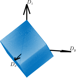
Dynamical Decoupling
<<ssec:detail_kinematics_cubic_dynamic>>
Introduction ignore
This section examines the dynamics of the cubic architecture in the Cartesian frame which corresponds to the transfer function from forces and torques $\bm{\mathcal{F}}$ to translations and rotations $\bm{\mathcal{X}}$ of the top platform. When relative motion sensors are integrated in each strut (measuring $\bm{\mathcal{L}}$), the pose $\bm{\mathcal{X}}$ is computed using the Jacobian matrix as shown in Figure ref:fig:detail_kinematics_centralized_control.
\begin{tikzpicture}
  \node[block] (Jt) at (0, 0) {$\bm{J}^{-T}$};
  \node[block, right= of Jt] (G) {$\bm{G}$};
  \node[block, right= of G] (J) {$\bm{J}^{-1}$};
  \node[block, left= of Jt] (Kx) {$\bm{K}_{\mathcal{X}}$};

  \draw[->] (Kx.east) -- node[midway, above]{$\bm{\mathcal{F}}$} (Jt.west);
  \draw[->] (Jt.east) -- (G.west) node[above left]{$\bm{\tau}$};
  \draw[->] (G.east) -- (J.west) node[above left]{$\bm{\mathcal{L}}$};
  \draw[->] (J.east) -- ++(1.0, 0);
  \draw[->] ($(J.east) + (0.5, 0)$)node[]{$\bullet$} node[above]{$\bm{\mathcal{X}}$} -- ++(0, -1) -| ($(Kx.west) + (-0.5, 0)$) -- (Kx.west);

  \begin{scope}[on background layer]
    \node[fit={(Jt.south west) (J.north east)}, fill=black!20!white, draw, dashed, inner sep=4pt] (Px) {};
    \node[anchor={south}] at (Px.north){\small{Cartesian Plant}};
  \end{scope}
\end{tikzpicture}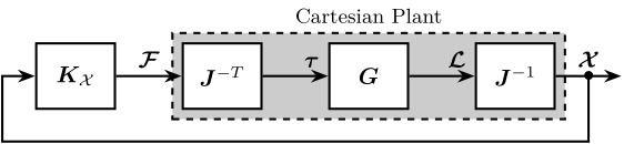
Low frequency and High frequency coupling
As derived during the conceptual design phase, the dynamics from $\bm{\mathcal{F}}$ to $\bm{\mathcal{X}}$ is described by Equation eqref:eq:detail_kinematics_transfer_function_cart. At low frequency, the behavior of the platform depends on the stiffness matrix eqref:eq:detail_kinematics_transfer_function_cart_low_freq.
\begin{equation}\label{eq:detail_kinematics_transfer_function_cart_low_freq} \frac{{\mathcal{X}}}{\bm{\mathcal{F}}}(j ω) \xrightarrow[ω → 0]{} \bm{K}-1
\end{equation}
In Section ref:ssec:detail_kinematics_cubic_static, it was demonstrated that for the cubic configuration, the stiffness matrix is diagonal if frame $\{B\}$ is positioned at the cube's center. In this case, the "Cartesian" plant is decoupled at low frequency. At high frequency, the behavior is governed by the mass matrix (evaluated at frame $\{B\}$) eqref:eq:detail_kinematics_transfer_function_high_freq.
\begin{equation}\label{eq:detail_kinematics_transfer_function_high_freq} \frac{{\mathcal{X}}}{\bm{\mathcal{F}}}(j ω) \xrightarrow[ω → ∞]{} - ω^2 \bm{M}-1
\end{equation}
To achieve a diagonal mass matrix, the center of mass of the mobile components must coincide with the $\{B\}$ frame, and the principal axes of inertia must align with the axes of the $\{B\}$ frame.
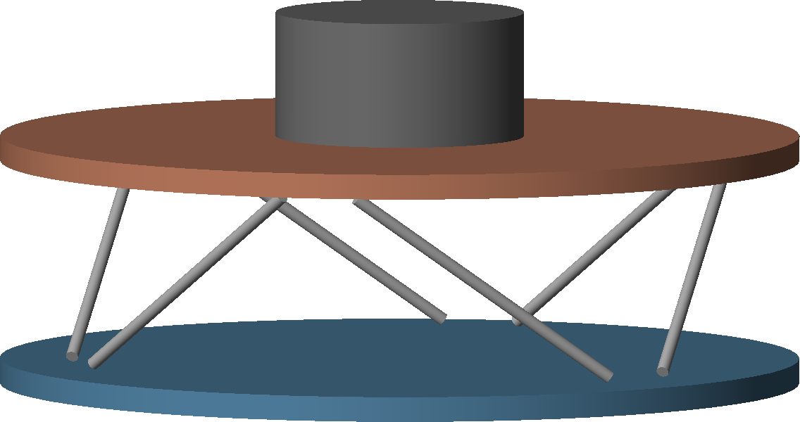
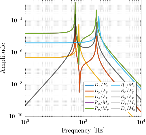
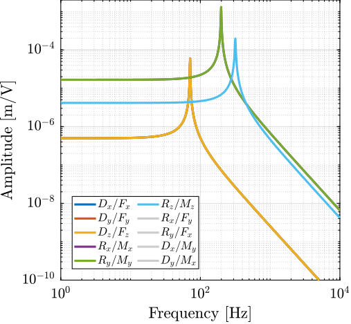
To verify these properties, a cubic Stewart platform with a cylindrical payload was analyzed (Figure ref:fig:detail_kinematics_cubic_payload). Transfer functions from $\bm{\mathcal{F}}$ to $\bm{\mathcal{X}}$ were computed for two specific locations of the $\{B\}$ frames. When the $\{B\}$ frame was positioned at the center of mass, coupling at low frequency was observed due to the non-diagonal stiffness matrix (Figure ref:fig:detail_kinematics_cubic_cart_coupling_com). Conversely, when positioned at the center of stiffness, coupling occurred at high frequency due to the non-diagonal mass matrix (Figure ref:fig:detail_kinematics_cubic_cart_coupling_cok).
%% Input/Output definition of the Simscape model
clear io; io_i = 1;
io(io_i) = linio([mdl, '/Controller'], 1, 'openinput');  io_i = io_i + 1; % Actuator Force Inputs [N]
io(io_i) = linio([mdl, '/plant'],      1, 'openoutput'); io_i = io_i + 1; % External metrology [m,rad]

% Prepare simulation
controller = initializeController('type', 'open-loop');
sample = initializeSample('type', 'cylindrical', 'm', 10, 'H', 100e-3, 'R', 100e-3);

%% Cubic Stewart platform with payload above the top platform - B frame at the CoM
H    = 200e-3; % height of the Stewart platform [m]
MO_B = 50e-3;  % Position {B} with respect to {M} [m]

stewart = initializeStewartPlatform();
stewart = initializeFramesPositions(stewart, 'H', H, 'MO_B', MO_B);
stewart = generateCubicConfiguration(stewart, 'Hc', H, 'FOc', H/2, 'FHa', 25e-3, 'MHb', 25e-3);
stewart = computeJointsPose(stewart);
stewart = initializeStrutDynamics(stewart, 'k', 1e6, 'c', 1e1);
stewart = initializeJointDynamics(stewart, 'type_F', '2dof', 'type_M', '3dof');
stewart = computeJacobian(stewart);
stewart = initializeStewartPose(stewart);
stewart = initializeCylindricalPlatforms(stewart, ...
                                         'Mpm', 1e-6, ... % Massless platform
                                         'Fpm', 1e-6, ... % Massless platform
                                         'Mph', 20e-3, ... % Thin platform
                                         'Fph', 20e-3, ... % Thin platform
                                         'Mpr', 1.2*max(vecnorm(stewart.platform_M.Mb)), ...
                                         'Fpr', 1.2*max(vecnorm(stewart.platform_F.Fa)));
stewart = initializeCylindricalStruts(stewart, ...
    'Fsm', 1e-6, ... % Massless strut
    'Msm', 1e-6, ... % Massless strut
    'Fsh', stewart.geometry.l(1)/2, ...
    'Msh', stewart.geometry.l(1)/2 ...
);

% Run the linearization
G_CoM = linearize(mdl, io)*inv(stewart.kinematics.J).';
G_CoM.InputName  = {'Fx', 'Fy', 'Fz', 'Mx', 'My', 'Mz'};
G_CoM.OutputName = {'Dx', 'Dy', 'Dz', 'Rx', 'Ry', 'Rz'};

%% Same geometry but B Frame at cube's center (CoK)
MO_B = -100e-3;  % Position {B} with respect to {M} [m]
stewart = initializeStewartPlatform();
stewart = initializeFramesPositions(stewart, 'H', H, 'MO_B', MO_B);
stewart = generateCubicConfiguration(stewart, 'Hc', H, 'FOc', H/2, 'FHa', 25e-3, 'MHb', 25e-3);
stewart = computeJointsPose(stewart);
stewart = initializeStrutDynamics(stewart, 'k', 1e6, 'c', 1e1);
stewart = initializeJointDynamics(stewart, 'type_F', '2dof', 'type_M', '3dof');
stewart = computeJacobian(stewart);
stewart = initializeStewartPose(stewart);
stewart = initializeCylindricalPlatforms(stewart, ...
                                         'Mpm', 1e-6, ... % Massless platform
                                         'Fpm', 1e-6, ... % Massless platform
                                         'Mph', 20e-3, ... % Thin platform
                                         'Fph', 20e-3, ... % Thin platform
                                         'Mpr', 1.2*max(vecnorm(stewart.platform_M.Mb)), ...
                                         'Fpr', 1.2*max(vecnorm(stewart.platform_F.Fa)));
stewart = initializeCylindricalStruts(stewart, ...
    'Fsm', 1e-6, ... % Massless strut
    'Msm', 1e-6, ... % Massless strut
    'Fsh', stewart.geometry.l(1)/2, ...
    'Msh', stewart.geometry.l(1)/2 ...
);

% Run the linearization
G_CoK = linearize(mdl, io)*inv(stewart.kinematics.J.');
G_CoK.InputName  = {'Fx', 'Fy', 'Fz', 'Mx', 'My', 'Mz'};
G_CoK.OutputName = {'Dx', 'Dy', 'Dz', 'Rx', 'Ry', 'Rz'};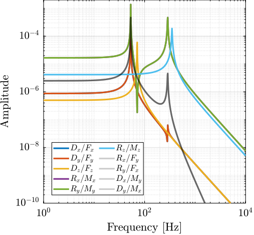
Payload's CoM at the cube's center
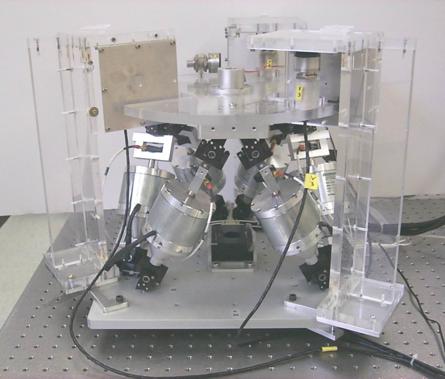
An effective strategy for improving dynamical performances involves aligning the cube's center (center of stiffness) with the center of mass of the moving components cite:&li01_simul_fault_vibrat_isolat_point. This can be achieved by positioning the payload below the top platform, such that the center of mass of the moving body coincides with the cube's center (Figure ref:fig:detail_kinematics_cubic_centered_payload). This approach was physically implemented in several studies cite:&mcinroy99_dynam;&jafari03_orthog_gough_stewar_platf_microm, as shown in Figure ref:fig:detail_kinematics_uw_gsp. The resulting dynamics are indeed well-decoupled (Figure ref:fig:detail_kinematics_cubic_cart_coupling_com_cok), taking advantage from diagonal stiffness and mass matrices. The primary limitation of this approach is that, for many applications including the nano-hexapod, the payload must be positioned above the top platform. If a design similar to Figure ref:fig:detail_kinematics_cubic_centered_payload were employed for the nano-hexapod, the X-ray beam would intersect with the struts during spindle rotation.
%% Cubic Stewart platform with payload above the top platform
H = 200e-3;
MO_B = -100e-3;  % Position {B} with respect to {M} [m]

stewart = initializeStewartPlatform();
stewart = initializeFramesPositions(stewart, 'H', H, 'MO_B', MO_B);
stewart = generateCubicConfiguration(stewart, 'Hc', H, 'FOc', H/2, 'FHa', 25e-3, 'MHb', 25e-3);
stewart = computeJointsPose(stewart);
stewart = initializeStrutDynamics(stewart, 'k', 1e6, 'c', 1e1);
stewart = initializeJointDynamics(stewart, 'type_F', '2dof', 'type_M', '3dof');
stewart = computeJacobian(stewart);
stewart = initializeStewartPose(stewart);
stewart = initializeCylindricalPlatforms(stewart, ...
                                         'Mpm', 1e-6, ... % Massless platform
                                         'Fpm', 1e-6, ... % Massless platform
                                         'Mph', 20e-3, ... % Thin platform
                                         'Fph', 20e-3, ... % Thin platform
                                         'Mpr', 1.2*max(vecnorm(stewart.platform_M.Mb)), ...
                                         'Fpr', 1.2*max(vecnorm(stewart.platform_F.Fa)));
stewart = initializeCylindricalStruts(stewart, ...
    'Fsm', 1e-6, ... % Massless strut
    'Msm', 1e-6, ... % Massless strut
    'Fsh', stewart.geometry.l(1)/2, ...
    'Msh', stewart.geometry.l(1)/2 ...
);

% Sample at the Center of the cube
sample = initializeSample('type', 'cylindrical', 'm', 10, 'H', 100e-3, 'H_offset', -H/2-50e-3);

% Run the linearization
G_CoM_CoK = linearize(mdl, io)*inv(stewart.kinematics.J.');
G_CoM_CoK.InputName  = {'Fx', 'Fy', 'Fz', 'Mx', 'My', 'Mz'};
G_CoM_CoK.OutputName = {'Dx', 'Dy', 'Dz', 'Rx', 'Ry', 'Rz'};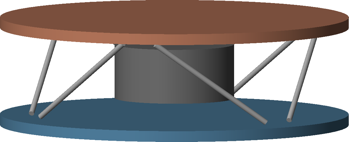
Conclusion
The analysis of dynamical properties of the cubic architecture yields several important conclusions. Static decoupling, characterized by a diagonal stiffness matrix, is achieved when reference frames $\{A\}$ and $\{B\}$ are positioned at the cube's center. Note that this property can also be obtained with non-cubic architectures that exhibit symmetrical strut arrangements. Dynamic decoupling requires both static decoupling and coincidence of the mobile platform's center of mass with reference frame $\{B\}$. While this configuration offers powerful control advantages, it requires positioning the payload at the cube's center, which is highly restrictive and often impractical.
Decentralized Control
<<ssec:detail_kinematics_decentralized_control>>
Introduction ignore
The orthogonal arrangement of struts in the cubic architecture suggests a potential minimization of inter-strut coupling, which could theoretically create favorable conditions for decentralized control. Two sensor types integrated in the struts are considered: displacement sensors and force sensors. The control architecture is illustrated in Figure ref:fig:detail_kinematics_decentralized_control, where $\bm{K}_{\mathcal{L}}$ represents a diagonal transfer function matrix.
\begin{tikzpicture}
  \node[block] (G) at (0,0) {$\bm{G}$};

  \node[block, left= of G] (Kl) {$\bm{K}_{\mathcal{L}}$};

  \draw[->] (Kl.east) -- node[midway, above]{$\bm{\tau}$} (G.west);
  \draw[->] (G.east) -- ++(1.0, 0);
  \draw[->] ($(G.east) + (0.5, 0)$)node[]{$\bullet$} node[above]{$\bm{\mathcal{L}}$} -- ++(0, -1) -| ($(Kl.west) + (-0.5, 0)$) -- (Kl.west);

  \begin{scope}[on background layer]
    \node[fit={(G.south west) (G.north east)}, fill=black!20!white, draw, dashed, inner sep=4pt] (Pl) {};
    \node[anchor={south}] at (Pl.north){\small{Strut Plant}};
  \end{scope}
\end{tikzpicture}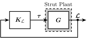
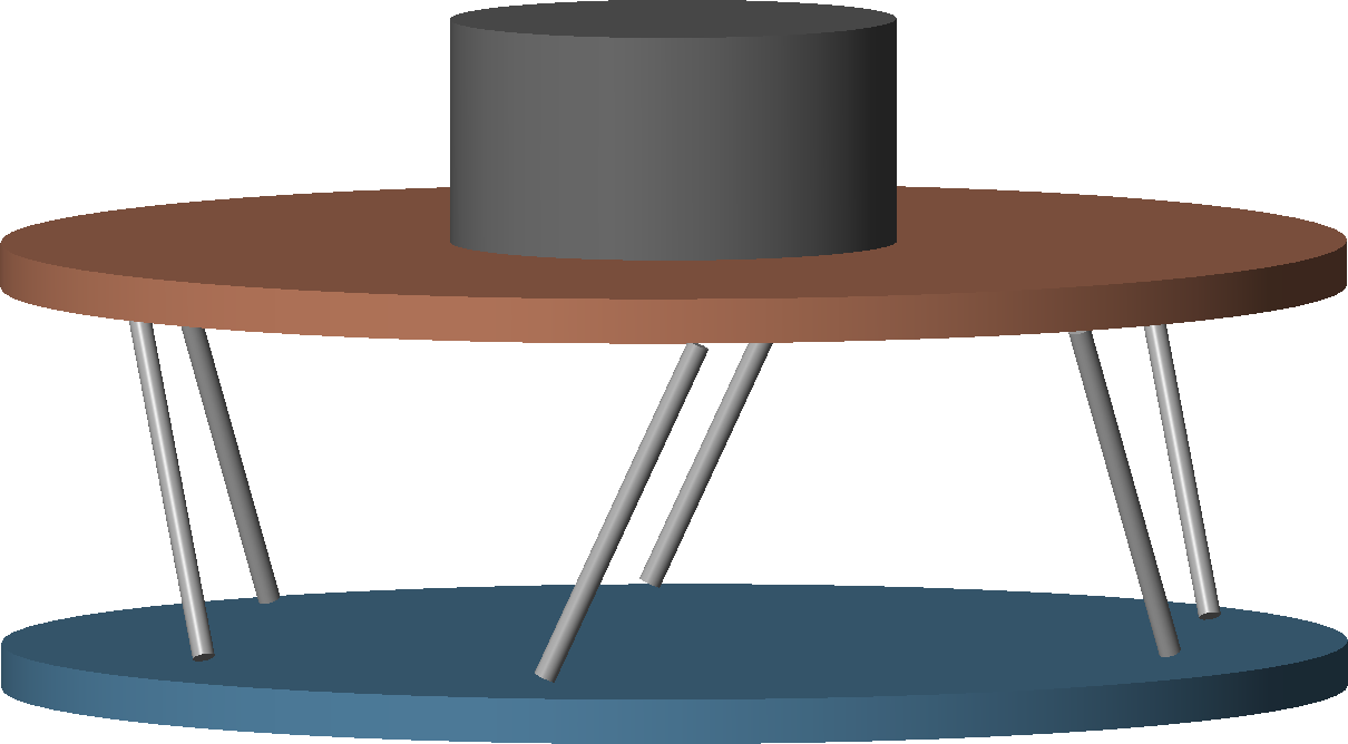
The obtained plant dynamics in the frame of the struts are compared for two Stewart platforms. The first employs a cubic architecture shown in Figure ref:fig:detail_kinematics_cubic_payload. The second uses a non-cubic Stewart platform shown in Figure ref:fig:detail_kinematics_non_cubic_payload, featuring identical payload and strut dynamics but with struts oriented more vertically to differentiate it from the cubic architecture.
%% Input/Output definition of the Simscape model
clear io; io_i = 1;
io(io_i) = linio([mdl, '/Controller'], 1, 'openinput');  io_i = io_i + 1; % Actuator Force Inputs [N]
io(io_i) = linio([mdl, '/plant'],      2, 'openoutput', [], 'dL'); io_i = io_i + 1; % Displacement sensors [m]
io(io_i) = linio([mdl, '/plant'],      2, 'openoutput', [], 'fn'); io_i = io_i + 1; % Force Sensor [N]

% Prepare simulation : Payload above the top platform
controller = initializeController('type', 'open-loop');
sample = initializeSample('type', 'cylindrical', 'm', 10, 'H', 100e-3, 'R', 100e-3);

%% Cubic Stewart platform
H    = 200e-3; % height of the Stewart platform [m]
MO_B = 50e-3;  % Position {B} with respect to {M} [m]

stewart = initializeStewartPlatform();
stewart = initializeFramesPositions(stewart, 'H', H, 'MO_B', MO_B);
stewart = generateCubicConfiguration(stewart, 'Hc', H, 'FOc', H/2, 'FHa', 25e-3, 'MHb', 25e-3);
stewart = computeJointsPose(stewart);
stewart = initializeStrutDynamics(stewart, 'k', 1e6, 'c', 1e1);
stewart = initializeJointDynamics(stewart, 'type_F', '2dof', 'type_M', '3dof');
stewart = computeJacobian(stewart);
stewart = initializeStewartPose(stewart);
stewart = initializeCylindricalPlatforms(stewart, ...
                                         'Mpm', 1e-6, ... % Massless platform
                                         'Fpm', 1e-6, ... % Massless platform
                                         'Mph', 20e-3, ... % Thin platform
                                         'Fph', 20e-3, ... % Thin platform
                                         'Mpr', 1.2*max(vecnorm(stewart.platform_M.Mb)), ...
                                         'Fpr', 1.2*max(vecnorm(stewart.platform_F.Fa)));
stewart = initializeCylindricalStruts(stewart, ...
    'Fsm', 1e-6, ... % Massless strut
    'Msm', 1e-6, ... % Massless strut
    'Fsh', stewart.geometry.l(1)/2, ...
    'Msh', stewart.geometry.l(1)/2 ...
);

% Run the linearization
G_cubic = linearize(mdl, io);
G_cubic.InputName  = {'f1', 'f2', 'f3', 'f4', 'f5', 'f6'};
G_cubic.OutputName = {'dL1', 'dL2', 'dL3', 'dL4', 'dL5', 'dL6', ...
                      'fn1', 'fn2', 'fn3', 'fn4', 'fn5', 'fn6'};

%% Non-Cubic Stewart platform
stewart = initializeStewartPlatform();
stewart = initializeFramesPositions(stewart, 'H', H, 'MO_B', MO_B);
stewart = generateCubicConfiguration(stewart, 'Hc', H, 'FOc', H/2, 'FHa', 25e-3, 'MHb', 25e-3);
stewart = generateGeneralConfiguration(stewart, 'FH', 25e-3, 'FR', 250e-3, 'MH', 25e-3, 'MR', 250e-3, ...
                                      'FTh', [-22, 22, 120-22, 120+22, 240-22, 240+22]*(pi/180), ...
                                      'MTh', [-60+22, 60-22, 60+22, 180-22, 180+22, -60-22]*(pi/180));
stewart = computeJointsPose(stewart);
stewart = initializeStrutDynamics(stewart, 'k', 1e6, 'c', 1e1);
stewart = initializeJointDynamics(stewart, 'type_F', '2dof', 'type_M', '3dof');
stewart = computeJacobian(stewart);
stewart = initializeStewartPose(stewart);
stewart = initializeCylindricalPlatforms(stewart, ...
                                         'Mpm', 1e-6, ... % Massless platform
                                         'Fpm', 1e-6, ... % Massless platform
                                         'Mph', 20e-3, ... % Thin platform
                                         'Fph', 20e-3, ... % Thin platform
                                         'Mpr', 1.2*max(vecnorm(stewart.platform_M.Mb)), ...
                                         'Fpr', 1.2*max(vecnorm(stewart.platform_F.Fa)));
stewart = initializeCylindricalStruts(stewart, ...
    'Fsm', 1e-6, ... % Massless strut
    'Msm', 1e-6, ... % Massless strut
    'Fsh', stewart.geometry.l(1)/2, ...
    'Msh', stewart.geometry.l(1)/2 ...
);

% Run the linearization
G_non_cubic = linearize(mdl, io);
G_non_cubic.InputName  = {'f1', 'f2', 'f3', 'f4', 'f5', 'f6'};
G_non_cubic.OutputName = {'dL1', 'dL2', 'dL3', 'dL4', 'dL5', 'dL6', ...
                          'fn1', 'fn2', 'fn3', 'fn4', 'fn5', 'fn6'};
Relative Displacement Sensors
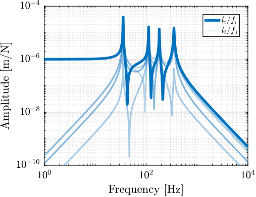
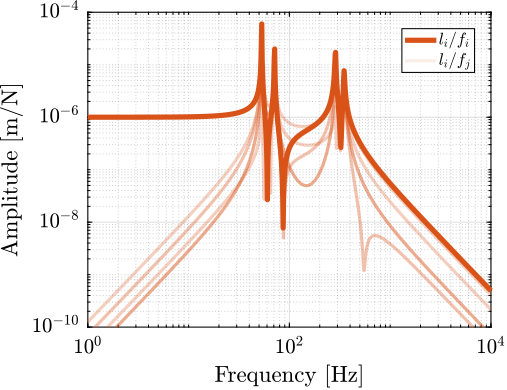
The transfer functions from actuator force in each strut to the relative motion of the struts are presented in Figure ref:fig:detail_kinematics_decentralized_dL. As anticipated from the equations of motion from $\bm{f}$ to $\bm{\mathcal{L}}$ eqref:eq:detail_kinematics_transfer_function_struts, the $6 \times 6$ plant is decoupled at low frequency. At high frequency, coupling is observed as the mass matrix projected in the strut frame is not diagonal.
No significant advantage is evident for the cubic architecture (Figure ref:fig:detail_kinematics_cubic_decentralized_dL) compared to the non-cubic architecture (Figure ref:fig:detail_kinematics_non_cubic_decentralized_dL). The resonance frequencies differ between the two cases because the more vertical strut orientation in the non-cubic architecture alters the stiffness properties of the Stewart platform, consequently shifting the frequencies of various modes.
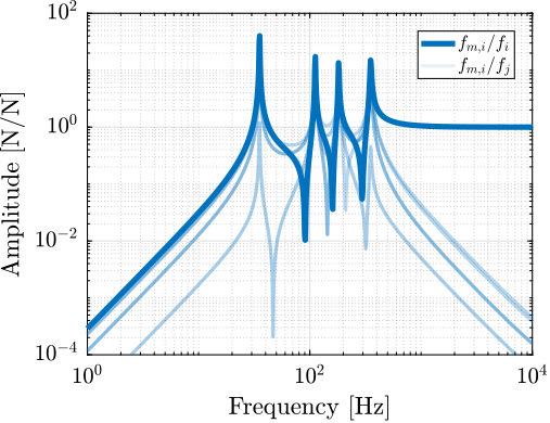
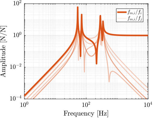
Force Sensors
Similarly, the transfer functions from actuator force to force sensors in each strut were analyzed for both cubic and non-cubic Stewart platforms. The results are presented in Figure ref:fig:detail_kinematics_decentralized_fn. The system demonstrates good decoupling at high frequency in both cases, with no clear advantage for the cubic architecture.
Conclusion
The presented results do not demonstrate the pronounced decoupling advantages often associated with cubic architectures in the literature. Both the cubic and non-cubic configurations exhibited similar coupling characteristics, suggesting that the benefits of orthogonal strut arrangement for decentralized control is less obvious than often reported in the literature.
Cubic architecture with Cube's center above the top platform
<<ssec:detail_kinematics_cubic_design>>
Introduction ignore
As demonstrated in Section ref:ssec:detail_kinematics_cubic_dynamic, the cubic architecture can exhibit advantageous dynamical properties when the center of mass of the moving body coincides with the cube's center, resulting in diagonal mass and stiffness matrices. As shown in Section ref:ssec:detail_kinematics_cubic_static, the stiffness matrix is diagonal when the considered $\{B\}$ frame is located at the cube's center. However, the $\{B\}$ frame is typically positioned above the top platform where forces are applied and displacements are measured.
This section proposes modifications to the cubic architecture to enable positioning the payload above the top platform while still leveraging the advantageous dynamical properties of the cubic configuration.
Three key parameters define the geometry of the cubic Stewart platform: $H$, the height of the Stewart platform (distance from fixed base to mobile platform); $H_c$, the height of the cube, as shown in Figure ref:fig:detail_kinematics_cubic_schematic_full; and $H_{CoM}$, the height of the center of mass relative to the mobile platform (coincident with the cube's center).
Depending on the cube's size $H_c$ in relation to $H$ and $H_{CoM}$, different designs emerge. In the following examples, $H = 100\,mm$ and $H_{CoM} = 20\,mm$.
%% Cubic configurations with center of the cube above the top platform
H    = 100e-3; % height of the Stewart platform [m]
MO_B = 20e-3;  % Position {B} with respect to {M} [m]
FOc  = H + MO_B; % Center of the cube with respect to {F}
Small cube
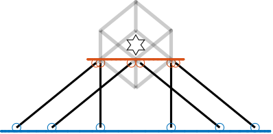
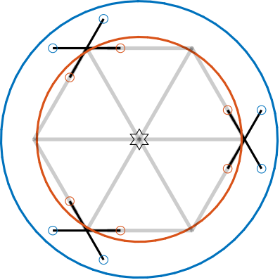
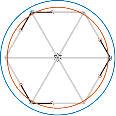
When the cube size $H_c$ is smaller than twice the height of the CoM $H_{CoM}$ eqref:eq:detail_kinematics_cube_small, the resulting design is shown in Figure ref:fig:detail_kinematics_cubic_above_small.
\begin{equation}\label{eq:detail_kinematics_cube_small} H_c < 2 HCoM
\end{equation}
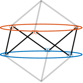
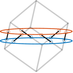
This configuration is similar to that described in cite:&furutani04_nanom_cuttin_machin_using_stewar, although they do not explicitly identify it as a cubic configuration. Adjacent struts are parallel to each other, differing from the typical architecture where parallel struts are positioned opposite to each other.
This approach yields a compact architecture, but the small cube size may result in insufficient rotational stiffness.
%% Small cube
Hc   = 2*MO_B;    % Size of the useful part of the cube [m]

stewart_small = initializeStewartPlatform();
stewart_small = initializeFramesPositions(stewart_small, 'H', H, 'MO_B', MO_B);
stewart_small = generateCubicConfiguration(stewart_small, 'Hc', Hc, 'FOc', FOc, 'FHa', 5e-3, 'MHb', 5e-3);
stewart_small = computeJointsPose(stewart_small);
stewart_small = initializeStrutDynamics(stewart_small, 'k', 1);
stewart_small = computeJacobian(stewart_small);
stewart_small = initializeCylindricalPlatforms(stewart_small, 'Fpr', 1.1*max(vecnorm(stewart_small.platform_F.Fa)), 'Mpr', 1.1*max(vecnorm(stewart_small.platform_M.Mb)));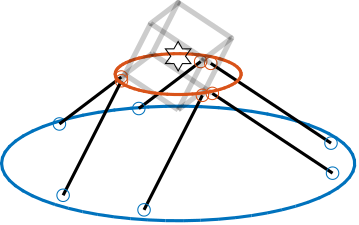
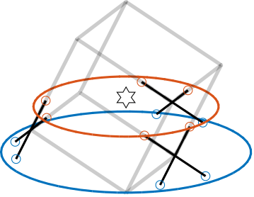
Medium sized cube
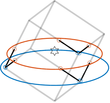
Increasing the cube's size such that eqref:eq:detail_kinematics_cube_medium is verified produces an architecture with intersecting struts (Figure ref:fig:detail_kinematics_cubic_above_medium).
\begin{equation}\label{eq:detail_kinematics_cube_medium} 2 HCoM < H_c < 2 (HCoM + H)
\end{equation}
This configuration resembles the design proposed in cite:&yang19_dynam_model_decoup_contr_flexib (Figure ref:fig:detail_kinematics_yang19), although their design is not strictly cubic.
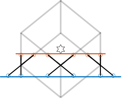
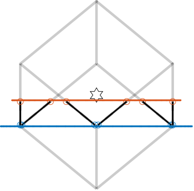
Large cube
When the cube's height exceeds twice the sum of the platform height and CoM height eqref:eq:detail_kinematics_cube_large, the architecture shown in Figure ref:fig:detail_kinematics_cubic_above_large is obtained.
\begin{equation}\label{eq:detail_kinematics_cube_large} 2 (HCoM + H) < H_c
\end{equation}
Platform size
%% Get the analytical formula for the location of the top and bottom joints
% Define symbolic variables
syms k Hc Hcom alpha H

assume(k > 0); % k is positive real
assume(Hcom > 0); % k is positive real
assume(Hc > 0); % Hc is real
assume(H > 0); % H is real
assume(alpha, 'real'); % alpha is real

% Define si matrix (edges of the cubes)
si = 1/sqrt(3)*[
  [ sqrt(2),    0,        1]; ...
  [-sqrt(2)/2, -sqrt(3/2), 1]; ...
  [-sqrt(2)/2,  sqrt(3/2), 1]; ...
  [ sqrt(2),    0,        1]; ...
  [-sqrt(2)/2, -sqrt(3/2), 1]; ...
  [-sqrt(2)/2,  sqrt(3/2), 1]  ...
];

% Define ci matrix (vertices of the cubes)
ci = Hc * [
  [1/sqrt(2), -sqrt(3)/sqrt(2), 0.5]; ...
  [1/sqrt(2), -sqrt(3)/sqrt(2), 0.5]; ...
  [1/sqrt(2),  sqrt(3)/sqrt(2), 0.5]; ...
  [1/sqrt(2),  sqrt(3)/sqrt(2), 0.5]; ...
  [-sqrt(2),   0,               0.5]; ...
  [-sqrt(2),   0,               0.5]  ...
];

% Apply vertical shift to ci
ci = ci + (H + Hcom) * [0, 0, 1];

% Calculate bi vectors (Stewart platform top joints)
bi = ci + alpha * si;


% Extract the z-component value from the first row of ci
% (all rows have the same z-component)
ci_z = ci(1, 3);

% The z-component of si is 1 for all rows
si_z = si(1, 3);

alpha_for_0 = solve(ci_z + alpha * si_z == 0, alpha);
alpha_for_H = solve(ci_z + alpha * si_z == H, alpha);

% Verify the results
% Substitute alpha values and check the resulting bi_z values
bi_z_0 = ci + alpha_for_0 * si;
disp('Radius for fixed base:');
simplify(sqrt(bi_z_0(1,1).^2 + bi_z_0(1,2).^2))

bi_z_H = ci + alpha_for_H * si;
disp('Radius for mobile platform:');
simplify(sqrt(bi_z_H(1,1).^2 + bi_z_H(1,2).^2))
For the proposed configuration, the top joints $\bm{b}_i$ (resp. the bottom joints $\bm{a}_i$) and are positioned on a circle with radius $R_{b_i}$ (resp. $R_{a_i}$) described by Equation eqref:eq:detail_kinematics_cube_joints.
\begin{subequations}\label{eq:detail_kinematics_cube_joints}
\begin{align} R_{b_i} &= \sqrt{\frac{3}{2} H_c^2 + 2 H_{CoM}^2} \label{eq:detail_kinematics_cube_top_joints} \\ R_{a_i} &= \sqrt{\frac{3}{2} H_c^2 + 2 (H_{CoM} + H)^2} \label{eq:detail_kinematics_cube_bot_joints} \end{align}\end{subequations}
Since the rotational stiffness for the cubic architecture scales with the square of the cube's height eqref:eq:detail_kinematics_cubic_stiffness, the cube's size can be determined based on rotational stiffness requirements. Subsequently, using Equation eqref:eq:detail_kinematics_cube_joints, the dimensions of the top and bottom platforms can be calculated.
Conclusion
The analysis of the cubic architecture for Stewart platforms yielded several important findings. While the cubic configuration provides uniform stiffness in the XYZ directions, it stiffness property becomes particularly advantageous when forces and torques are applied at the cube's center. Under these conditions, the stiffness matrix becomes diagonal, resulting in a decoupled Cartesian plant at low frequencies.
Regarding mobility, the translational capabilities of the cubic configuration exhibit uniformity along the directions of the orthogonal struts, rather than complete uniformity in the Cartesian space. This understanding refines the characterization of cubic architecture mobility commonly presented in literature.
The analysis of decentralized control in the frame of the struts revealed more nuanced results than expected. While cubic architectures are frequently associated with reduced coupling between actuators and sensors, this study showed that these benefits may be more subtle or context-dependent than commonly described. Under the conditions analyzed, the coupling characteristics of cubic and non-cubic configurations, in the frame of the struts, appeared similar.
Fully decoupled dynamics in the Cartesian frame can be achieved when the center of mass of the moving body coincides with the cube's center. However, this arrangement presents practical challenges, as the cube's center is traditionally located between the top and bottom platforms, making payload placement problematic for many applications.
To address this limitation, modified cubic architectures have been proposed with the cube's center positioned above the top platform. Three distinct configurations have been identified, each with different geometric arrangements but sharing the common characteristic that the cube's center is positioned above the top platform. This structural modification enables the alignment of the moving body's center of mass with the center of stiffness, resulting in beneficial decoupling properties in the Cartesian frame.
Nano Hexapod
<<sec:detail_kinematics_nano_hexapod>>
Introduction ignore
Based on previous analysis, this section aims to determine the nano-hexapod optimal geometry. For the NASS, the chosen reference frames $\{A\}$ and $\{B\}$ coincide with the sample's point of interest, which is positioned $150\,mm$ above the top platform. This is the location where precise control of the sample's position is required, as it is where the x-ray beam is focused.
Requirements
<<ssec:detail_kinematics_nano_hexapod_requirements>>
The design of the nano-hexapod must satisfy several constraints. The device should fit within a cylinder with radius of $120\,mm$ and height of $95\,mm$. Based on the measured errors of all stages of the micro-stations, and incorporating safety margins, the required mobility should enable combined translations in any direction of $\pm 50\,\mu m$. At any position, the system should be capable of performing $R_x$ and $R_y$ rotations of $\pm 50\,\mu \text{rad}$. Regarding stiffness, the resonance frequencies should be well above the maximum rotational velocity of $2\pi\,\text{rad/s}$ to minimize gyroscopic effects, while remaining below the problematic modes of the micro-station to ensure decoupling from its complex dynamics. In terms of dynamics, the design should facilitate implementation of Integral Force Feedback (IFF) in a decentralized manner, and provide good decoupling for the high authority controller in the frame of the struts.
Obtained Geometry
<<ssec:detail_kinematics_nano_hexapod_geometry>>
Based on the previous analysis of Stewart platform configurations, while the geometry can be optimized to achieve the desired trade-off between stiffness and mobility in different directions, the wide range of potential payloads, with masses ranging from 1kg to 50kg, makes it impossible to develop a single geometry that provides optimal dynamical properties for all possible configurations.
For the nano-hexapod design, the struts were oriented more vertically compared to a cubic architecture due to several considerations. First, the performance requirements in the vertical direction are more stringent than in the horizontal direction. This vertical strut orientation decreases the amplification factor in the vertical direction, providing greater resolution and reducing the effects of actuator noise. Second, the micro-station's vertical modes exhibit higher frequencies than its lateral modes. Therefore, higher resonance frequencies of the nano-hexapod in the vertical direction compared to the horizontal direction enhance the decoupling properties between the micro-station and the nano-hexapod.
Regarding dynamical properties, particularly for control in the frame of the struts, no specific optimization was implemented since the analysis revealed that strut orientation has minimal impact on the resulting coupling characteristics.
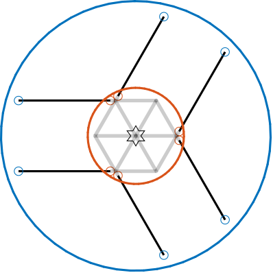
Consequently, the geometry was selected according to practical constraints. The height between the two plates is maximized and set at $95\,mm$. Both platforms utilize the maximum available size, with joints offset by $15\,mm$ from the plate surfaces and positioned along circles with radii of $120\,mm$ for the fixed joints and $110\,mm$ for the mobile joints. The positioning angles, as shown in Figure ref:fig:detail_kinematics_nano_hexapod_top, are $[255,\ 285,\ 15,\ 45,\ 135,\ 165]$ degrees for the top joints and $[220,\ 320,\ 340,\ 80,\ 100,\ 200]$ degrees for the bottom joints.
%% Obtained Nano Hexapod Design
nano_hexapod = initializeStewartPlatform();
nano_hexapod = initializeFramesPositions(nano_hexapod, ...
                                    'H', 95e-3, ...
                                    'MO_B', 150e-3);

nano_hexapod = generateGeneralConfiguration(nano_hexapod, ...
                                       'FH', 15e-3, ...
                                       'FR', 120e-3, ...
                                       'FTh', [220, 320, 340, 80, 100, 200]*(pi/180), ...
                                       'MH', 15e-3, ...
                                       'MR', 110e-3, ...
                                       'MTh', [255, 285, 15, 45, 135, 165]*(pi/180));
nano_hexapod = computeJointsPose(nano_hexapod);
nano_hexapod = initializeStrutDynamics(nano_hexapod, 'k', 1);
nano_hexapod = computeJacobian(nano_hexapod);
nano_hexapod = initializeCylindricalPlatforms(nano_hexapod, 'Fpr', 125e-3, 'Mpr', 115e-3);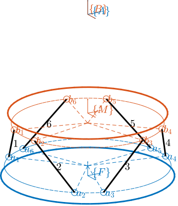
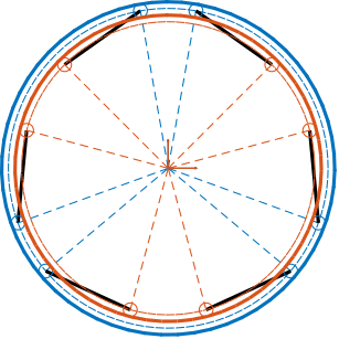
The resulting geometry is illustrated in Figure ref:fig:detail_kinematics_nano_hexapod. While minor refinements may occur during detailed mechanical design to address manufacturing and assembly considerations, the fundamental geometry will remain consistent with this configuration. This geometry serves as the foundation for estimating required actuator stroke (Section ref:ssec:detail_kinematics_nano_hexapod_actuator_stroke), determining flexible joint stroke requirements (Section ref:ssec:detail_kinematics_nano_hexapod_joint_stroke), performing noise budgeting for instrumentation selection, and developing control strategies.
Implementing a cubic architecture as proposed in Section ref:ssec:detail_kinematics_cubic_design was considered. However, positioning the cube's center $150\,mm$ above the top platform would have resulted in platform dimensions exceeding the maximum available size. Additionally, to benefit from the cubic configuration's dynamical properties, each payload would require careful calibration of inertia before placement on the nano-hexapod, ensuring that its center of mass coincides with the cube's center. Given the impracticality of consistently aligning the center of mass with the cube's center, the cubic architecture was deemed unsuitable for the nano-hexapod application.
Required Actuator stroke
<<ssec:detail_kinematics_nano_hexapod_actuator_stroke>>
With the geometry established, the actuator stroke necessary to achieve the desired mobility can be determined.
The required mobility parameters include combined translations in the XYZ directions of $\pm 50\,\mu m$ (essentially a cubic workspace). Additionally, at any point within this workspace, combined $R_x$ and $R_y$ rotations of $\pm 50\,\mu \text{rad}$, with $R_z$ maintained at 0, should be possible.
Calculations based on the selected geometry indicate that an actuator stroke of $\pm 94\,\mu m$ is required to achieve the desired mobility. This specification will be used during the actuator selection process.
Figure ref:fig:detail_kinematics_nano_hexapod_mobility illustrates both the desired mobility (represented as a cube) and the calculated mobility envelope of the nano-hexapod with an actuator stroke of $\pm 94\,\mu m$. The diagram confirms that the required workspace fits within the system's capabilities.
%% Estimate required actuator stroke for the wanted mobility
max_translation = 50e-6; % Wanted translation mobility [m]
max_rotation = 50e-6; % Wanted rotation mobility [rad]

Dxs = linspace(-max_translation, max_translation, 3);
Dys = linspace(-max_translation, max_translation, 3);
Dzs = linspace(-max_translation, max_translation, 3);
Rxs = linspace(-max_rotation, max_rotation, 3);
Rys = linspace(-max_rotation, max_rotation, 3);

L_min = 0; % Required actuator negative stroke [m]
L_max = 0; % Required actuator negative stroke [m]

for Dx = Dxs
    for Dy = Dys
        for Dz = Dzs
            for Rx = Rxs
                for Ry = Rys
                    ARB = [ cos(Ry) 0        sin(Ry);
                            0       1        0;
                           -sin(Ry) 0        cos(Ry)] * ...
                          [ 1       0        0;
                            0       cos(Rx) -sin(Rx);
                            0       sin(Rx)  cos(Rx)];

                    [~, Ls] = inverseKinematics(nano_hexapod, 'AP', [Dx;Dy;Dz], 'ARB', ARB);

                    if min(Ls) < L_min
                        L_min = min(Ls);
                    end
                    if max(Ls) > L_max
                        L_max = max(Ls);
                    end
                end
            end
        end
    end
end

sprintf('Actuator stroke should be from %.0f um to %.0f um', 1e6*L_min, 1e6*L_max)
%% Compute mobility in translation with combined angular motion
% Direction of motion (spherical coordinates)
thetas = linspace(0, pi, 100);
phis = linspace(0, 2*pi, 100);
% Considered Rotations
Rxs = linspace(-max_rotation, max_rotation, 3);
Rys = linspace(-max_rotation, max_rotation, 3);
% Maximum distance that can be reached in the direction of motion
% Considering combined angular motion and limited actuator stroke
rs = zeros(length(thetas), length(phis));
worst_rx_ry = zeros(length(thetas), length(phis), 2);
for i = 1:length(thetas)
for j = 1:length(phis)
% Compute unitary motion in the considered direction
Tx = sin(thetas(i))*cos(phis(j));
Ty = sin(thetas(i))*sin(phis(j));
Tz = cos(thetas(i));
% Start without considering rotations
dL_lin = nano_hexapod.kinematics.J*[Tx; Ty; Tz; 0; 0; 0];
% Strut motion for maximum displacement in the considered direction
dL_lin_max = L_max*dL_lin/max(abs(dL_lin));
% Find rotation that gives worst case stroke
dL_worst = max(abs(dL_lin_max)); % This should be equal to L_max
dL_rot_max = zeros(6,1);
% Perform (small) rotations, and find the (worst) case requiring maximum strut motion
for Rx = Rxs
for Ry = Rys
dL_rot = nano_hexapod.kinematics.J*[0; 0; 0; Rx; Ry; 0];
if max(abs(dL_lin_max + dL_rot)) > dL_worst
dL_worst = max(abs(dL_lin_max + dL_rot));
dL_rot_max = dL_rot;
worst_rx_ry(i,j,:) = [Rx, Ry];
end
end
end
stroke_ratio = min(abs([( L_max - dL_rot_max) ./ dL_lin_max; (-L_max - dL_rot_max) ./ dL_lin_max]));
dL_real = dL_lin_max*stroke_ratio + dL_rot_max;
% % Obtained maximum displacement in the considered direction with angular motion
rs(i, j) = stroke_ratio*L_max/max(abs(dL_lin));
end
end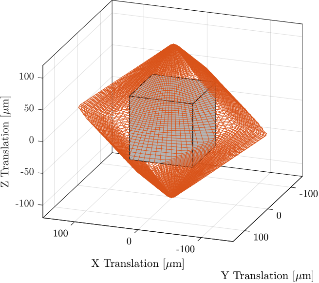
Required Joint angular stroke
<<ssec:detail_kinematics_nano_hexapod_joint_stroke>>
With the nano-hexapod geometry and mobility requirements established, the flexible joint angular stroke necessary to avoid limiting the achievable workspace can be determined.
This analysis focuses solely on bending stroke, as the torsional stroke of the flexible joints is expected to be minimal given the absence of vertical rotation requirements. The required angular stroke for both fixed and mobile joints is estimated to be equal to $1\,\text{mrad}$. This specification will guide the design of the flexible joints.
%% Estimate required actuator stroke for the wanted mobility
max_translation = 50e-6; % Wanted translation mobility [m]
max_rotation = 50e-6; % Wanted rotation mobility [rad]

Dxs = linspace(-max_translation, max_translation, 3);
Dys = linspace(-max_translation, max_translation, 3);
Dzs = linspace(-max_translation, max_translation, 3);
Rxs = linspace(-max_rotation, max_rotation, 3);
Rys = linspace(-max_rotation, max_rotation, 3);

max_angles_F = zeros(1,6); % Maximum bending angle - Fixed joints [rad]
max_angles_M = zeros(1,6); % Maximum bending angle - Mobile joints [rad]

% Compute initial strut orientation
nano_hexapod = computeJointsPose(nano_hexapod, 'AP', zeros(3,1), 'ARB', eye(3));
As = nano_hexapod.geometry.As; % Fixed joints
Bs = nano_hexapod.geometry.Bs; % Mobile joints

for Dx = Dxs
    for Dy = Dys
        for Dz = Dzs
            for Rx = Rxs
                for Ry = Rys
                    ARB = [ cos(Ry) 0        sin(Ry);
                            0       1        0;
                           -sin(Ry) 0        cos(Ry)] * ...
                          [ 1       0        0;
                            0       cos(Rx) -sin(Rx);
                            0       sin(Rx)  cos(Rx)];

                    nano_hexapod = computeJointsPose(nano_hexapod, 'AP', [Dx;Dy;Dz], 'ARB', ARB);

                    angles_M = acos(dot(Bs, nano_hexapod.geometry.Bs));
                    max_angles_M(angles_M > max_angles_M) = angles_M(angles_M > max_angles_M);

                    angles_F = acos(dot(Bs, nano_hexapod.geometry.As));
                    max_angles_F(angles_F > max_angles_F) = angles_F(angles_F > max_angles_F);
                end
            end
        end
    end
end

sprintf('Fixed joint stroke should be %.1f mrad', 1e3*max(max_angles_F))
sprintf('Mobile joint stroke should be %.1f mrad', 1e3*max(max_angles_M))
Conclusion
<<sec:detail_kinematics_conclusion>>
This chapter has explored the optimization of the nano-hexapod geometry for the Nano Active Stabilization System (NASS).
First, a review of existing Stewart platforms revealed two main geometric categories: cubic architectures, characterized by mutually orthogonal struts arranged along the edges of a cube, and non-cubic architectures with varied strut orientations. While cubic architectures are prevalent in the literature and attributed with beneficial properties such as simplified kinematics, uniform stiffness, and reduced cross-coupling, the performed analysis revealed that some of these advantages should be more nuanced or context-dependent than commonly described.
The analytical relationships between Stewart platform geometry and its mechanical properties were established, enabling a better understanding of the trade-offs between competing requirements such as mobility and stiffness along different axes. These insights were useful during the nano-hexapod geometry optimization.
For the cubic configuration, complete dynamical decoupling in the Cartesian frame can be achieved when the center of mass of the moving body coincides with the cube's center, but this arrangement is often impractical for real-world applications. Modified cubic architectures with the cube's center positioned above the top platform were proposed as a potential solution, but proved unsuitable for the nano-hexapod due to size constraints and the impracticality of ensuring that different payloads' centers of mass would consistently align with the cube's center.
For the nano-hexapod design, a key challenge was addressing the wide range of potential payloads (1 to 50kg), which made it impossible to optimize the geometry for consistent dynamic performance across all usage scenarios. This led to a practical design approach where struts were oriented more vertically than in cubic configurations to address several application-specific needs: achieving higher resolution in the vertical direction by reducing amplification factors and better matching the micro-station's modal characteristics with higher vertical resonance frequencies.