phd-nass-geometry/nass-geometry.org

Nano Hexapod - Optimal Geometry

• Introduction
• Review of Stewart platforms
  • Introduction
• Effect of geometry on Stewart platform properties
  • Introduction
  • Platform Mobility / Workspace
    • Introduction
    • Mobility in translation
    • Mobility in rotation
    • Combined translations and rotations
  • Stiffness
    • Introduction
    • Translation Stiffness
    • Rotational Stiffness
    • Diagonal Stiffness Matrix
  • Dynamical properties
    • In the Cartesian Frame
    • In the frame of the Struts
    • Dynamic Isotropy
  • Conclusion
• The Cubic Architecture
  • Introduction
  • Static Properties
    • Stiffness matrix for the Cubic architecture
    • Effect of having frame $\{B\}$ off-centered
    • Uniform Mobility
  • Dynamical Decoupling
    • Introduction
    • Low frequency and High frequency coupling
    • Payload's CoM at the cube's center
    • Conclusion
  • Decentralized Control
    • Introduction
    • Relative Displacement Sensors
    • Force Sensors
    • Conclusion
  • Cubic architecture with Cube's center above the top platform
    • Introduction
    • Small cube
    • Medium sized cube
    • Large cube
    • Platform size
    • Conclusion
  • Conclusion
• Nano Hexapod
  • Introduction
  • Obtained Geometry
  • Required Actuator stroke
  • Required Joint angular stroke
• Conclusion
• Bibliography

Introduction   ignore

• In the conceptual design phase, the geometry of the Stewart platform was chosen arbitrarily and not optimized
• In the detail design phase, we want to see if the geometry can be optimized to improve the overall performances
• Optimization criteria: mobility, stiffness, dynamical decoupling, more performance / bandwidth

Outline:

• Review of Stewart platform (Section ref:sec:detail_kinematics_stewart_review) Geometry, Actuators, Sensors, Joints
• Effect of geometry on the Stewart platform characteristics (Section ref:sec:detail_kinematics_geometry)
• Cubic configuration: benefits? (Section ref:sec:detail_kinematics_cubic)
• Obtained geometry for the nano hexapod (Section ref:sec:detail_kinematics_nano_hexapod)

Review of Stewart platforms

<<sec:detail_kinematics_stewart_review>>

Introduction   ignore

• As was explained in the conceptual phase, Stewart platform have the following key elements:

  • Two plates connected by six struts

  • Each strut is composed of:

    • a flexible joint at each end
    • an actuator
    • one or several sensors
• The exact geometry (i.e. position of joints and orientation of the struts) can be chosen freely depending on the application.
• This results in many different designs found in the literature.
• The focus is here made on Stewart platforms for nano-positioning and vibration control. Long stroke stewart platforms are not considered here as their design impose other challenges. Some Stewart platforms found in the literature are listed in Table ref:tab:detail_kinematics_stewart_review
• All presented Stewart platforms are using flexible joints, as it is a prerequisites for nano-positioning capabilities.

• Most of stewart platforms are using voice coil actuators or piezoelectric actuators. The actuators used for the Stewart platform will be chosen in the next section.

• Depending on the application, various sensors are integrated in the struts or on the plates. The choice of sensor for the nano-hexapod will be described in the next section.

• There are two categories of Stewart platform geometry:

  • Cubic architecture (Figure ref:fig:detail_kinematics_stewart_examples_cubic). Struts are positioned along 6 sides of a cubic (and are therefore orthogonal to each other). Such specific architecture has some special properties that will be studied in Section ref:sec:detail_kinematics_cubic.
  • Non-cubic architecture (Figure ref:fig:detail_kinematics_stewart_examples_non_cubic)

\bigskip

\bigskip

	Geometry	Actuators	Sensors	Reference
	Cubic	Magnetostrictive	Force, Accelerometers	cite:&geng93_six_degree_of_freed_activ;&geng94_six_degree_of_freed_activ;&geng95_intel_contr_system_multip_degree
Figure ref:fig:detail_kinematics_jpl	Cubic	Voice Coil (0.5 mm)	Force	cite:&spanos95_soft_activ_vibrat_isolat;&rahman98_multiax
	Cubic	Voice Coil (10 mm)	Force, LVDT, Geophones	cite:&thayer98_stewar;&thayer02_six_axis_vibrat_isolat_system;&hauge04_sensor_contr_space_based_six
Figure ref:fig:detail_kinematics_uw_gsp	Cubic	Voice Coil	Force	cite:&mcinroy99_dynam;&mcinroy99_precis_fault_toler_point_using_stewar_platf;&mcinroy00_desig_contr_flexur_joint_hexap;&li01_simul_vibrat_isolat_point_contr;&jafari03_orthog_gough_stewar_platf_microm
	Cubic	Piezoelectric ($25\,\mu m$)	Force	cite:&defendini00_techn
Figure ref:fig:detail_kinematics_ulb_pz	Cubic	APA ($50\,\mu m$)	Force	cite:&abu02_stiff_soft_stewar_platf_activ
Figure ref:fig:detail_kinematics_pph	Non-Cubic	Voice Coil	Accelerometers	cite:&chen03_payload_point_activ_vibrat_isolat
	Cubic	Voice Coil	Force	cite:&hanieh03_activ_stewar;&preumont07_six_axis_singl_stage_activ
Figure ref:fig:detail_kinematics_uqp	Cubic	Piezoelectric ($50\,\mu m$)	Geophone	cite:&agrawal04_algor_activ_vibrat_isolat_spacec
	Non-Cubic	Piezoelectric ($16\,\mu m$)	Eddy Current	cite:&furutani04_nanom_cuttin_machin_using_stewar
	Cubic	Piezoelectric ($120\,\mu m$)	(External) Capacitive	cite:&ting06_desig_stewar_nanos_platf;&ting13_compos_contr_desig_stewar_nanos_platf
	Non-Cubic	Piezoelectric ($160\,\mu m$)	(External) Capacitive	cite:&ting07_measur_calib_stewar_microm_system
Figure ref:fig:detail_kinematics_zhang11	Non-cubic	Magnetostrictive	Accelerometer	cite:&zhang11_six_dof
	Non-Cubic	Piezoelectric	Strain Gauge	cite:&du14_piezo_actuat_high_precis_flexib
	Cubic	Voice Coil	Accelerometer	cite:&chi15_desig_exper_study_vcm_based;&tang18_decen_vibrat_contr_voice_coil;&jiao18_dynam_model_exper_analy_stewar
	Cubic	Piezoelectric	Force	cite:&wang16_inves_activ_vibrat_isolat_stewar
	Almost cubic	Voice Coil	Force, Accelerometer	cite:&beijen18_self_tunin_mimo_distur_feedf;&tjepkema12_activ_ph
Figure ref:fig:detail_kinematics_yang19	Almost cubic	Piezoelectric	Force, Strain gauge	cite:&yang19_dynam_model_decoup_contr_flexib
Figure ref:fig:detail_kinematics_naves	Non-Cubic	3-phase rotary motor	Rotary Encoder	cite:&naves20_desig;&naves20_t_flex

Conclusion:

• Various Stewart platform designs:

  • geometry, sizes, orientation of struts
  • Lot's have a "cubic" architecture that will be discussed in Section ref:sec:detail_kinematics_cubic
  • actuator types
  • various sensors
  • flexible joints (discussed in next chapter)
• The effect of geometry on the properties of the Stewart platform is studied in section ref:sec:detail_kinematics_geometry
• It is determined what is the optimal geometry for the NASS

Effect of geometry on Stewart platform properties

<<sec:detail_kinematics_geometry>>

Introduction   ignore

• As was shown during the conceptual phase, the geometry of the Stewart platform influences:

  • the stiffness and compliance properties
  • the mobility
  • the force authority
  • the dynamics of the manipulator
• It is therefore important to understand how the geometry impact these properties, and to be able to optimize the geometry for a specific application.

One important tool to study this is the Jacobian matrix which depends on the $\bm{b}_i$ (join position w.r.t top platform) and $\hat{\bm{s}}_i$ (orientation of struts). The choice of frames ($\{A\}$ and $\{B\}$), independently of the physical Stewart platform geometry, impacts the obtained kinematics and stiffness matrix, as it is defined for forces and motion evaluated at the chosen frame.

Platform Mobility / Workspace

Introduction   ignore

The mobility of the Stewart platform (or any manipulator) is here defined as the range of motion that it can perform. It corresponds to the set of possible pose (i.e. combined translation and rotation) of frame {B} with respect to frame {A}. It should therefore be represented in a six dimensional space.

As was shown during the conceptual phase, for small displacements, the Jacobian matrix can be used to link the strut motion to the motion of frame B with respect to A through equation eqref:eq:detail_kinematics_jacobian.

\begin{equation}\label{eq:detail_kinematics_jacobian} \begin{bmatrix} \delta l_1 \\ \delta l_2 \\ \delta l_3 \\ \delta l_4 \\ \delta l_5 \\ \delta l_6 \end{bmatrix} = \begin{bmatrix} {{}^A\hat{\bm{s}}_1}^T & ({}^A\bm{b}_1 \times {}^A\hat{\bm{s}}_1)^T \\ {{}^A\hat{\bm{s}}_2}^T & ({}^A\bm{b}_2 \times {}^A\hat{\bm{s}}_2)^T \\ {{}^A\hat{\bm{s}}_3}^T & ({}^A\bm{b}_3 \times {}^A\hat{\bm{s}}_3)^T \\ {{}^A\hat{\bm{s}}_4}^T & ({}^A\bm{b}_4 \times {}^A\hat{\bm{s}}_4)^T \\ {{}^A\hat{\bm{s}}_5}^T & ({}^A\bm{b}_5 \times {}^A\hat{\bm{s}}_5)^T \\ {{}^A\hat{\bm{s}}_6}^T & ({}^A\bm{b}_6 \times {}^A\hat{\bm{s}}_6)^T \end{bmatrix} \begin{bmatrix} \delta x \\ \delta y \\ \delta z \\ \delta \theta_x \\ \delta \theta_y \\ \delta \theta_z \end{bmatrix} = \begin{bmatrix} {{}^A\hat{\bm{s}}_1}^T & ({}^A\bm{b}_1 \times {}^A\hat{\bm{s}}_1)^T \\ {{}^A\hat{\bm{s}}_2}^T & ({}^A\bm{b}_2 \times {}^A\hat{\bm{s}}_2)^T \\ {{}^A\hat{\bm{s}}_3}^T & ({}^A\bm{b}_3 \times {}^A\hat{\bm{s}}_3)^T \\ {{}^A\hat{\bm{s}}_4}^T & ({}^A\bm{b}_4 \times {}^A\hat{\bm{s}}_4)^T \\ {{}^A\hat{\bm{s}}_5}^T & ({}^A\bm{b}_5 \times {}^A\hat{\bm{s}}_5)^T \\ {{}^A\hat{\bm{s}}_6}^T & ({}^A\bm{b}_6 \times {}^A\hat{\bm{s}}_6)^T \end{bmatrix} \begin{bmatrix} \delta x \\ \delta y \\ \delta z \\ \delta \theta_x \\ \delta \theta_y \\ \delta \theta_z \end{bmatrix} \begin{bmatrix} \delta x \\ \delta y \\ \delta z \\ \delta \theta_x \\ \delta \theta_y \\ \delta \theta_z \end{bmatrix}

\end{equation}

Therefore, the mobility of the Stewart platform (set of $[\delta x\ \delta y\ \delta z\ \delta \theta_x\ \delta \theta_y\ \delta \theta_z]$) depends on:

• the stroke of each strut
• the geometry of the Stewart platform (embodied in the Jacobian matrix)

More specifically:

• the XYZ mobility only depends on the si (orientation of struts)
• the mobility in rotation depends on bi (position of top joints)

As will be shown in Section ref:sec:detail_kinematics_cubic, there are some geometry that gives same stroke in X, Y and Z directions.

As the mobility is of dimension six, it is difficult to represent. Depending on the applications, only the translation mobility or the rotation mobility may be represented.

Although there is no human readable way to represent the complete workspace, some projections of the full workspace can be drawn.

Difficulty of studying workspace of parallel manipulators.

Mobility in translation

Here, for simplicity, only translations are first considered:

• Let's consider a general Stewart platform geometry shown in Figure ref:fig:detail_kinematics_mobility_trans_arch.
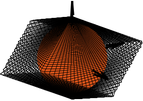
• In the general case: the translational mobility can be represented by a 3D shape with 12 faces (each actuator limits the stroke along its orientation in positive and negative directions). The faces are therefore perpendicular to the strut direction. The obtained mobility is shown in Figure ref:fig:detail_kinematics_mobility_trans_result.
• Considering an actuator stroke of $\pm d$, the mobile platform can be translated in any direction with a stroke of $d$ A circle with radius $d$ can be contained in the general shape. It will touch the shape along six lines defined by the strut axes. The sphere with radius $d$ is shown in Figure ref:fig:detail_kinematics_mobility_trans_result.
• Therefore, for any (small stroke) Stewart platform with actuator stroke $\pm d$, it is possible to move the top platform in any direction by at least a distance $d$. Note that no platform angular motion is here considered. When combining angular motion, the linear stroke decreases.
• When considering some symmetry in the system (as typically the case), the shape becomes a Trigonal trapezohedron whose height and width depends on the orientation of the struts. We only get 6 faces as usually the Stewart platform consists of 3 sets of 2 parallels struts.
• In reality, portion of spheres, but well approximated by flat surfaces for short stroke hexapods.

thetas = linspace(0, pi, 100);
phis = linspace(0, 2*pi, 100);
rs = zeros(length(thetas), length(phis));

for i = 1:length(thetas)
    for j = 1:length(phis)
        Tx = sin(thetas(i))*cos(phis(j));
        Ty = sin(thetas(i))*sin(phis(j));
        Tz = cos(thetas(i));

        dL = stewart.kinematics.J*[Tx; Ty; Tz; 0; 0; 0;]; % dL required for 1m displacement in theta/phi direction

        rs(i, j) = L_max/max(abs(dL));
    end
end

% Sphere with radius equal to actuator stroke
[Xs,Ys,Zs] = sphere;
Xs = 1e6*L_max*Xs;
Ys = 1e6*L_max*Ys;
Zs = 1e6*L_max*Zs;

[phi_grid, theta_grid] = meshgrid(phis, thetas);
X = 1e6 * rs .* sin(theta_grid) .* cos(phi_grid);
Y = 1e6 * rs .* sin(theta_grid) .* sin(phi_grid);
Z = 1e6 * rs .* cos(theta_grid);

figure('Renderer', 'painters');
hold on;
surf(X,  Y,  Z,  'FaceColor', 'none', 'LineWidth', 0.1, 'EdgeColor', [0, 0, 0]);
surf(Xs, Ys, Zs, 'FaceColor', colors(2,:), 'EdgeColor', 'none');
quiver3(0, 0, 0, 100, 0, 0, 'k', 'LineWidth', 2, 'MaxHeadSize', 0.9);
quiver3(0, 0, 0, 0, 100, 0, 'k', 'LineWidth', 2, 'MaxHeadSize', 0.9);
quiver3(0, 0, 0, 0, 0, 100, 'k', 'LineWidth', 2, 'MaxHeadSize', 0.9);
hold off;
axis equal;
grid off;
axis off;
view(55, 25);

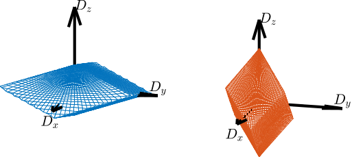
To better understand how the geometry of the Stewart platform impacts the translational mobility, two configurations are compared:

• Struts oriented horizontally (Figure ref:fig:detail_kinematics_stewart_mobility_vert_struts) => more stroke in horizontal direction
• Struts oriented vertically (Figure ref:fig:detail_kinematics_stewart_mobility_hori_struts) => more stroke in vertical direction
• Corresponding mobility shown in Figure ref:fig:detail_kinematics_mobility_translation_strut_orientation

Mobility in rotation

As shown by equation eqref:eq:detail_kinematics_jacobian, the rotational mobility depends both on the orientation of the struts and on the location of the top joints.

Similarly to the translational case, to increase the rotational mobility in one direction, it is advantageous to have the struts more perpendicular to the rotational direction.

For instance, having the struts more vertical (Figure ref:fig:detail_kinematics_stewart_mobility_vert_struts) gives less rotational stroke along the vertical direction than having the struts oriented more horizontally (Figure ref:fig:detail_kinematics_stewart_mobility_hori_struts).

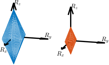
Two cases are considered with same strut orientation but with different top joints positions:

• struts close to each other (Figure ref:fig:detail_kinematics_stewart_mobility_close_struts)
• struts further apart (Figure ref:fig:detail_kinematics_stewart_mobility_space_struts)

The mobility for pure rotations are compared in Figure ref:fig:detail_kinematics_mobility_angle_strut_distance. Note that the same strut stroke are considered in both cases to evaluate the mobility. Having struts further apart decreases the "level arm" and therefore the rotational mobility is reduced.

For rotations and translations, having more mobility also means increasing the effect of actuator noise on the considering degree of freedom. Somehow, the level arm is increased, so any strut vibration gets amplified. Therefore, the designed Stewart platform should just have the necessary mobility.

Combined translations and rotations

It is possible to consider combined translations and rotations. Displaying such mobility is more complex. It will be used for the nano-hexapod to verify that the obtained design has the necessary mobility.

For a fixed geometry and a wanted mobility (combined translations and rotations), it is possible to estimate the required minimum actuator stroke. It will be done in Section ref:sec:detail_kinematics_nano_hexapod to estimate the required actuator stroke for the nano-hexapod geometry.

Stiffness

Introduction   ignore

Stiffness matrix:

• defines how the nano-hexapod deforms (frame $\{B\}$ with respect to frame $\{A\}$) due to static forces/torques applied on $\{B\}$.
• Depends on the Jacobian matrix (i.e. the geometry) and the strut axial stiffness eqref:eq:detail_kinematics_stiffness_matrix
• Contribution of joints stiffness is here not considered cite:&mcinroy00_desig_contr_flexur_joint_hexap;&mcinroy02_model_desig_flexur_joint_stewar

\begin{equation}\label{eq:detail_kinematics_stiffness_matrix} \bm{K} = \bm{J}^T \bm{\mathcal{K}} \bm{J}

\end{equation}

It is assumed that the stiffness of all strut is the same: $\bm{\mathcal{K}} = k \cdot \mathbf{I}_6$. Obtained stiffness matrix linearly depends on the strut stiffness $k$ eqref:eq:detail_kinematics_stiffness_matrix_simplified.

\begin{equation}\label{eq:detail_kinematics_stiffness_matrix_simplified} \bm{K} = k \bm{J}^T \bm{J} = k ≤ft[ \begin{array}{c|c} Σ_{i = 0}⁶ \hat{\bm{s}}_i ⋅ \hat{\bm{s}}_i^T & Σ_{i = 0}⁶ \bm{\hat{s}}_i ⋅ ({}^A\bm{b}_i × {}^A\hat{\bm{s}}_i)^T
\hline Σ_{i = 0}⁶ ({}^A\bm{b}_i × {}^A\hat{\bm{s}}_i) ⋅ \hat{\bm{s}}_i^T & Σ_{i = 0}⁶ ({}^A\bm{b}_i × {}^A\hat{\bm{s}}_i) ⋅ ({}^A\bm{b}_i × {}^A\hat{\bm{s}}_i)^T\\

\end{array} \right]

\end{equation}

Translation Stiffness

XYZ stiffnesses:

• Only depends on the orientation of the struts and not their location: $\hat{\bm{s}}_i \cdot \hat{\bm{s}}_i^T$
• Extreme case: all struts are vertical $s_i = [0,\ 0,\ 1]$ => vertical stiffness of $6 k$, but null stiffness in X and Y directions
• If two struts along X, two struts along Y, and two struts along Z => $\hat{\bm{s}}_i \cdot \hat{\bm{s}}_i^T = 2 \bm{I}_3$ Stiffness is well distributed along directions. This corresponds to the cubic architecture.

If struts more vertical (Figure ref:fig:detail_kinematics_stewart_mobility_vert_struts):

• increase vertical stiffness
• decrease horizontal stiffness
• increase Rx,Ry stiffness
• decrease Rz stiffness

Opposite conclusions if struts are not horizontal (Figure ref:fig:detail_kinematics_stewart_mobility_hori_struts).

Rotational Stiffness

Rotational stiffnesses:

• Same orientation but increased distances (bi) by a factor 2 => rotational stiffness increased by factor 4 Figure ref:fig:detail_kinematics_stewart_mobility_close_struts Figure ref:fig:detail_kinematics_stewart_mobility_space_struts

Struts further apart:

• no change to XYZ
• increase in rotational stiffness (by the square of the distance)

Diagonal Stiffness Matrix

Having the stiffness matrix $\bm{K}$ diagonal can be beneficial for control purposes as it would make the plant in the cartesian frame decoupled at low frequency.

This depends on the geometry and on the chosen {A} frame.

For specific configurations, it is possible to have a diagonal K matrix.

This will be discussed in Section ref:ssec:detail_kinematics_cubic_static.

Dynamical properties

In the Cartesian Frame

Dynamical equations (both in the cartesian frame and in the frame of the struts) for the Stewart platform were derived during the conceptual phase with simplifying assumptions (massless struts and perfect joints).

The dynamics depends both on the geometry (Jacobian matrix) but also on the payload being placed on top of the platform.

Under very specific conditions, the equations of motion can be decoupled in the Cartesian space. These are studied in Section ref:ssec:detail_kinematics_cubic_dynamic.

\begin{equation}\label{eq:nhexa_transfer_function_cart} \frac{{\mathcal{X}}}{\bm{\mathcal{F}}}(s) = ( \bm{M} s^2 + \bm{J}^T \bm{\mathcal{C}} \bm{J} s + \bm{J}^T \bm{\mathcal{K}} \bm{J} )^-1

\end{equation}

In the frame of the Struts

In the frame of the struts, the equations of motion are well decoupled at low frequency. This is why most of Stewart platforms are controlled in the frame of the struts: bellow the resonance frequency, the system is decoupled and SISO control may be applied for each strut.

\begin{equation}\label{eq:nhexa_transfer_function_struts} \frac{\bm{\mathcal{L}}}{\bm{f}}(s) = ( \bm{J}^-T \bm{M} \bm{J}^-1 s^2 + \bm{\mathcal{C}} + \bm{\mathcal{K}} )^-1

\end{equation}

Coupling between sensors (force sensors, relative position sensor, inertial sensors) in different struts may also be important for decentralized control. Can the geometry be optimized to have lower coupling between the struts? This will be studied with the cubic architecture.

TODO Dynamic Isotropy

cite:&afzali-far16_vibrat_dynam_isotr_hexap_analy_studies: "Dynamic isotropy, leading to equal eigenfrequencies, is a powerful optimization measure."

Conclusion

The effects of two changes in the manipulator's geometry, namely the position and orientation of the legs, are summarized in Table ref:tab:detail_kinematics_geometry. These results could have been easily deduced based on some mechanical principles, but thanks to the kinematic analysis, they can be quantified.

These trade-offs give some guidelines when choosing the Stewart platform geometry.

	legs pointing more vertically	legs further apart
Vertical stiffness	$\nearrow$	$=$
Horizontal stiffness	$\searrow$	$=$
Vertical rotation stiffness	$\searrow$	$\nearrow$
Horizontal rotation stiffness	$\nearrow$	$\nearrow$
Vertical force authority	$\nearrow$	$=$
Horizontal force authority	$\searrow$	$=$
Vertical torque authority	$\searrow$	$\nearrow$
Horizontal torque authority	$\nearrow$	$\nearrow$
Vertical stroke	$\searrow$	$=$
Horizontal stroke	$\nearrow$	$=$
Vertical rotation stroke	$\nearrow$	$\searrow$
Horizontal rotation stroke	$\searrow$	$\searrow$

Effect of a change in geometry on the manipulator's stiffness, force authority and stroke

The Cubic Architecture

<<sec:detail_kinematics_cubic>>

Introduction   ignore

The Cubic configuration for the Stewart platform was first proposed in cite:&geng94_six_degree_of_freed_activ.

This configuration is quite specific in the sense that the active struts are arranged in a mutually orthogonal configuration connecting the corners of a cube Figure ref:fig:detail_kinematics_cubic_architecture_examples.

Cubic configuration:

• The struts are corresponding to 6 of the 8 edges of a cube.
• This way, all struts are perpendicular to each other (except sets of two that are parallel).

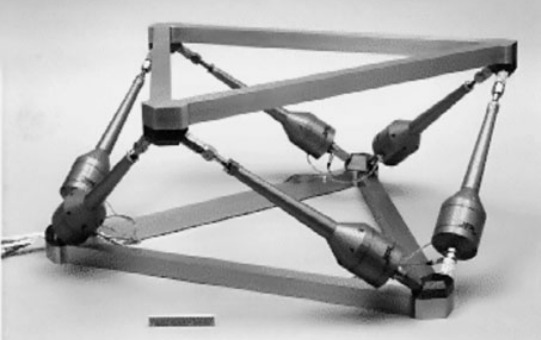
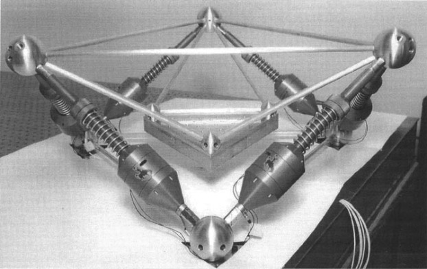
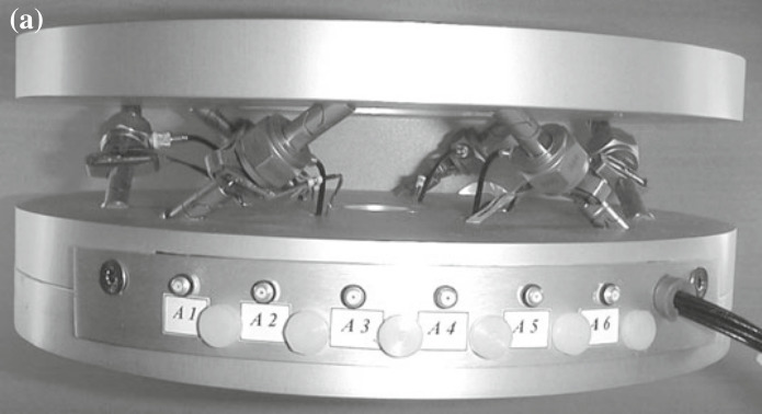
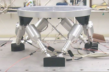
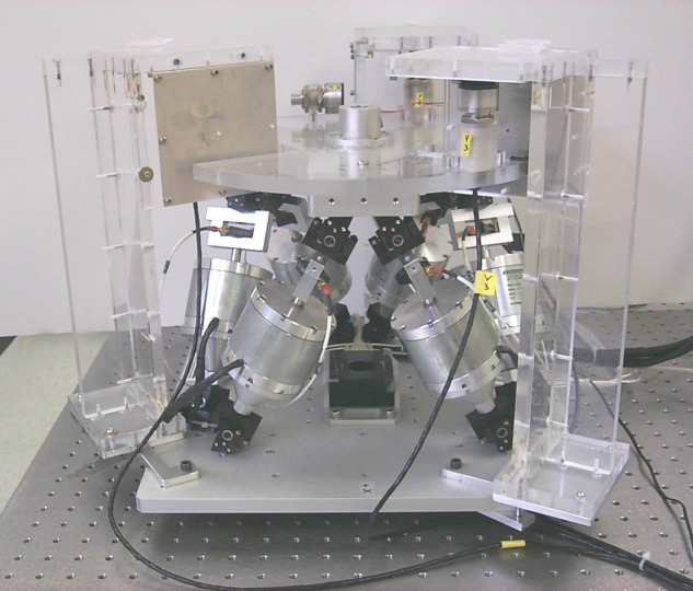
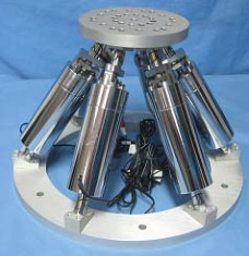
Struts with similar size than the cube's edge (Figure ref:fig:detail_kinematics_cubic_architecture_example). Similar to Figures ref:fig:detail_kinematics_jpl, ref:fig:detail_kinematics_uw_gsp and ref:fig:detail_kinematics_uqp.

Struts smaller than the cube's edge (Figure ref:fig:detail_kinematics_cubic_architecture_example_small). Similar to the Stewart platform of Figure ref:fig:detail_kinematics_ulb_pz.

The cubic configuration is attributed a number of properties that made this configuration widely used (cite:&preumont07_six_axis_singl_stage_activ;&jafari03_orthog_gough_stewar_platf_microm). From cite:&geng94_six_degree_of_freed_activ:

1. Uniformity in control capability in all directions
2. Uniformity in stiffness in all directions
3. Minimum cross coupling force effect among actuators
4. Facilitate collocated sensor-actuator control system design
5. Simple kinematics relationships
6. Simple dynamic analysis
7. Simple mechanical design

According to cite:&preumont07_six_axis_singl_stage_activ, it "minimizes the cross-coupling amongst actuators and sensors of different legs" (being orthogonal to each other).

Specific points of interest are:

• uniform mobility, uniform stiffness, and coupling properties

In this section:

• Such properties are studied
• Additional properties interesting for control?
• It is determined if the cubic architecture is interested for the nano-hexapod

Static Properties

<<ssec:detail_kinematics_cubic_static>>

Stiffness matrix for the Cubic architecture

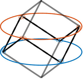
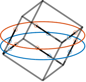
Consider the cubic architecture shown in Figure ref:fig:detail_kinematics_cubic_schematic_full.

The unit vectors corresponding to the edges of the cube are described by eqref:eq:detail_kinematics_cubic_s.

\begin{equation}\label{eq:detail_kinematics_cubic_s} \hat{\bm{s}}_1 = \begin{bmatrix} \sqrt{2}/\sqrt{3} \\ 0 \\ 1/\sqrt{3} \end{bmatrix} \quad \hat{\bm{s}}_2 = \begin{bmatrix} -1/\sqrt{6} \\ -1/\sqrt{2} \\ 1/\sqrt{3} \end{bmatrix} \quad \hat{\bm{s}}_3 = \begin{bmatrix} -1/\sqrt{6} \\ 1/\sqrt{2} \\ 1/\sqrt{3} \end{bmatrix} \quad \hat{\bm{s}}_4 = \begin{bmatrix} \sqrt{2}/\sqrt{3} \\ 0 \\ 1/\sqrt{3} \end{bmatrix} \quad \hat{\bm{s}}_5 = \begin{bmatrix} -1/\sqrt{6} \\ -1/\sqrt{2} \\ 1/\sqrt{3} \end{bmatrix} \quad \hat{\bm{s}}_6 = \begin{bmatrix} -1/\sqrt{6} \\ 1/\sqrt{2} \\ 1/\sqrt{3} \end{bmatrix} \quad \hat{\bm{s}}_2 = \begin{bmatrix} -1/\sqrt{6} \\ -1/\sqrt{2} \\ 1/\sqrt{3} \end{bmatrix} \quad \hat{\bm{s}}_3 = \begin{bmatrix} -1/\sqrt{6} \\ 1/\sqrt{2} \\ 1/\sqrt{3} \end{bmatrix} \quad \hat{\bm{s}}_4 = \begin{bmatrix} \sqrt{2}/\sqrt{3} \\ 0 \\ 1/\sqrt{3} \end{bmatrix} \quad \hat{\bm{s}}_5 = \begin{bmatrix} -1/\sqrt{6} \\ -1/\sqrt{2} \\ 1/\sqrt{3} \end{bmatrix} \quad \hat{\bm{s}}_6 = \begin{bmatrix} -1/\sqrt{6} \\ 1/\sqrt{2} \\ 1/\sqrt{3} \end{bmatrix} \quad \hat{\bm{s}}_3 = \begin{bmatrix} -1/\sqrt{6} \\ 1/\sqrt{2} \\ 1/\sqrt{3} \end{bmatrix} \quad \hat{\bm{s}}_4 = \begin{bmatrix} \sqrt{2}/\sqrt{3} \\ 0 \\ 1/\sqrt{3} \end{bmatrix} \quad \hat{\bm{s}}_5 = \begin{bmatrix} -1/\sqrt{6} \\ -1/\sqrt{2} \\ 1/\sqrt{3} \end{bmatrix} \quad \hat{\bm{s}}_6 = \begin{bmatrix} -1/\sqrt{6} \\ 1/\sqrt{2} \\ 1/\sqrt{3} \end{bmatrix} \quad \hat{\bm{s}}_4 = \begin{bmatrix} \sqrt{2}/\sqrt{3} \\ 0 \\ 1/\sqrt{3} \end{bmatrix} \quad \hat{\bm{s}}_5 = \begin{bmatrix} -1/\sqrt{6} \\ -1/\sqrt{2} \\ 1/\sqrt{3} \end{bmatrix} \quad \hat{\bm{s}}_6 = \begin{bmatrix} -1/\sqrt{6} \\ 1/\sqrt{2} \\ 1/\sqrt{3} \end{bmatrix} \quad \hat{\bm{s}}_5 = \begin{bmatrix} -1/\sqrt{6} \\ -1/\sqrt{2} \\ 1/\sqrt{3} \end{bmatrix} \quad \hat{\bm{s}}_6 = \begin{bmatrix} -1/\sqrt{6} \\ 1/\sqrt{2} \\ 1/\sqrt{3} \end{bmatrix} \quad \hat{\bm{s}}_6 = \begin{bmatrix} -1/\sqrt{6} \\ 1/\sqrt{2} \\ 1/\sqrt{3} \end{bmatrix}

\end{equation}

Coordinates of the cube's vertices relevant for the top joints, expressed with respect to the cube's center eqref:eq:detail_kinematics_cubic_vertices.

\begin{equation}\label{eq:detail_kinematics_cubic_vertices} ~{\bm{b}}_1 = ~{\bm{b}}_2 = H_c \begin{bmatrix} \frac{1}{\sqrt{2}} \\ \frac{-\sqrt{3}}{\sqrt{2}} \\ \frac{1}{2} \end{bmatrix}, \quad \tilde{\bm{b}}_3 = \tilde{\bm{b}}_4 = H_c \begin{bmatrix} \frac{1}{\sqrt{2}} \\ \frac{ \sqrt{3}}{\sqrt{2}} \\ \frac{1}{2} \end{bmatrix}, \quad \tilde{\bm{b}}_5 = \tilde{\bm{b}}_6 = H_c \begin{bmatrix} \frac{-2}{\sqrt{2}} \\ 0 \\ \frac{1}{2} \end{bmatrix}, \quad ~{\bm{b}}_3 = ~{\bm{b}}_4 = H_c \begin{bmatrix} \frac{1}{\sqrt{2}} \\ \frac{ \sqrt{3}}{\sqrt{2}} \\ \frac{1}{2} \end{bmatrix}, \quad \tilde{\bm{b}}_5 = \tilde{\bm{b}}_6 = H_c \begin{bmatrix} \frac{-2}{\sqrt{2}} \\ 0 \\ \frac{1}{2} \end{bmatrix}, \quad ~{\bm{b}}_5 = ~{\bm{b}}_6 = H_c \begin{bmatrix} \frac{-2}{\sqrt{2}} \\ 0 \\ \frac{1}{2} \end{bmatrix}

\end{equation}

  \begin{tikzpicture}
    \begin{scope}[rotate={45}, shift={(0, 0, -4)}]
      % We first define the coordinate of the points of the Cube
      \coordinate[] (bot) at (0,0,4);
      \coordinate[] (top) at (4,4,0);
      \coordinate[] (A1) at (0,0,0);
      \coordinate[] (A2) at (4,0,4);
      \coordinate[] (A3) at (0,4,4);
      \coordinate[] (B1) at (4,0,0);
      \coordinate[] (B2) at (4,4,4);
      \coordinate[] (B3) at (0,4,0);

      % Center of the Cube
      \node[] (cubecenter) at ($0.5*(bot) + 0.5*(top)$){$\bullet$};

      % We draw parts of the cube that corresponds to the Stewart platform
      \draw[] (A1)node[]{$\bullet$} -- (B1)node[]{$\bullet$} -- (A2)node[]{$\bullet$} -- (B2)node[]{$\bullet$} -- (A3)node[]{$\bullet$} -- (B3)node[]{$\bullet$} -- (A1);

      % ai and bi are computed
      \def\lfrom{0.0}
      \def\lto{1.0}

      \coordinate(a1) at ($(A1) - \lfrom*(A1) + \lfrom*(B1)$);
      \coordinate(b1) at ($(A1) - \lto*(A1)   + \lto*(B1)$);
      \coordinate(a2) at ($(A2) - \lfrom*(A2) + \lfrom*(B1)$);
      \coordinate(b2) at ($(A2) - \lto*(A2)   + \lto*(B1)$);
      \coordinate(a3) at ($(A2) - \lfrom*(A2) + \lfrom*(B2)$);
      \coordinate(b3) at ($(A2) - \lto*(A2)   + \lto*(B2)$);
      \coordinate(a4) at ($(A3) - \lfrom*(A3) + \lfrom*(B2)$);
      \coordinate(b4) at ($(A3) - \lto*(A3)   + \lto*(B2)$);
      \coordinate(a5) at ($(A3) - \lfrom*(A3) + \lfrom*(B3)$);
      \coordinate(b5) at ($(A3) - \lto*(A3)   + \lto*(B3)$);
      \coordinate(a6) at ($(A1) - \lfrom*(A1) + \lfrom*(B3)$);
      \coordinate(b6) at ($(A1) - \lto*(A1)   + \lto*(B3)$);

      % We draw the fixed and mobiles platforms
      \path[fill=colorblue, opacity=0.2] (a1) -- (a2) -- (a3) -- (a4) -- (a5) -- (a6) -- cycle;
      \path[fill=colorblue, opacity=0.2] (b1) -- (b2) -- (b3) -- (b4) -- (b5) -- (b6) -- cycle;
      \draw[color=colorblue, dashed] (a1) -- (a2) -- (a3) -- (a4) -- (a5) -- (a6) -- cycle;
      \draw[color=colorblue, dashed] (b1) -- (b2) -- (b3) -- (b4) -- (b5) -- (b6) -- cycle;

      % The legs of the hexapod are drawn
      \draw[color=colorblue] (a1)node{$\bullet$} -- (b1)node{$\bullet$};
      \draw[color=colorblue] (a2)node{$\bullet$} -- (b2)node{$\bullet$};
      \draw[color=colorblue] (a3)node{$\bullet$} -- (b3)node{$\bullet$};
      \draw[color=colorblue] (a4)node{$\bullet$} -- (b4)node{$\bullet$};
      \draw[color=colorblue] (a5)node{$\bullet$} -- (b5)node{$\bullet$};
      \draw[color=colorblue] (a6)node{$\bullet$} -- (b6)node{$\bullet$};

      % Unit vector
      \draw[color=colorred, ->] ($0.9*(a1)+0.1*(b1)$)node{$\bullet$} -- ($0.65*(a1)+0.35*(b1)$)node[right]{$\hat{\bm{s}}_3$};
      \draw[color=colorred, ->] ($0.9*(a2)+0.1*(b2)$)node{$\bullet$} -- ($0.65*(a2)+0.35*(b2)$)node[left]{$\hat{\bm{s}}_4$};
      \draw[color=colorred, ->] ($0.9*(a3)+0.1*(b3)$)node{$\bullet$} -- ($0.65*(a3)+0.35*(b3)$)node[below]{$\hat{\bm{s}}_5$};
      \draw[color=colorred, ->] ($0.9*(a4)+0.1*(b4)$)node{$\bullet$} -- ($0.65*(a4)+0.35*(b4)$)node[below]{$\hat{\bm{s}}_6$};
      \draw[color=colorred, ->] ($0.9*(a5)+0.1*(b5)$)node{$\bullet$} -- ($0.65*(a5)+0.35*(b5)$)node[left]{$\hat{\bm{s}}_1$};
      \draw[color=colorred, ->] ($0.9*(a6)+0.1*(b6)$)node{$\bullet$} -- ($0.65*(a6)+0.35*(b6)$)node[right]{$\hat{\bm{s}}_2$};

      % Labels
      \node[above=0.1 of B1] {$\tilde{\bm{b}}_3 = \tilde{\bm{b}}_4$};
      \node[above=0.1 of B2] {$\tilde{\bm{b}}_5 = \tilde{\bm{b}}_6$};
      \node[above=0.1 of B3] {$\tilde{\bm{b}}_1 = \tilde{\bm{b}}_2$};
    \end{scope}

    % Height of the Hexapod
    \coordinate[] (sizepos) at ($(a2)+(0.2, 0)$);
    \coordinate[] (origin) at (0,0,0);

    \draw[->] (cubecenter.center) node[above right]{$\{B\}$} -- ++(0,0,1);
    \draw[->] (cubecenter.center) -- ++(1,0,0);
    \draw[->] (cubecenter.center) -- ++(0,1,0);

    % Useful part of the cube
    \draw[<->, dashed] ($(A2)+(0.5,0)$) -- node[midway, right]{$H_{C}$} ($(B1)+(0.5,0)$);
  \end{tikzpicture}

  \begin{tikzpicture}
    \begin{scope}[rotate={45}, shift={(0, 0, -4)}]
      % We first define the coordinate of the points of the Cube
      \coordinate[] (bot) at (0,0,4);
      \coordinate[] (top) at (4,4,0);
      \coordinate[] (A1) at (0,0,0);
      \coordinate[] (A2) at (4,0,4);
      \coordinate[] (A3) at (0,4,4);
      \coordinate[] (B1) at (4,0,0);
      \coordinate[] (B2) at (4,4,4);
      \coordinate[] (B3) at (0,4,0);

      % Center of the Cube
      \node[] (cubecenter) at ($0.5*(bot) + 0.5*(top)$){$\bullet$};

      % We draw parts of the cube that corresponds to the Stewart platform
      \draw[] (A1)node[]{$\bullet$} -- (B1)node[]{$\bullet$} -- (A2)node[]{$\bullet$} -- (B2)node[]{$\bullet$} -- (A3)node[]{$\bullet$} -- (B3)node[]{$\bullet$} -- (A1);

      % ai and bi are computed
      \def\lfrom{0.2}
      \def\lto{0.8}

      \coordinate(a1) at ($(A1) - \lfrom*(A1) + \lfrom*(B1)$);
      \coordinate(b1) at ($(A1) - \lto*(A1)   + \lto*(B1)$);
      \coordinate(a2) at ($(A2) - \lfrom*(A2) + \lfrom*(B1)$);
      \coordinate(b2) at ($(A2) - \lto*(A2)   + \lto*(B1)$);
      \coordinate(a3) at ($(A2) - \lfrom*(A2) + \lfrom*(B2)$);
      \coordinate(b3) at ($(A2) - \lto*(A2)   + \lto*(B2)$);
      \coordinate(a4) at ($(A3) - \lfrom*(A3) + \lfrom*(B2)$);
      \coordinate(b4) at ($(A3) - \lto*(A3)   + \lto*(B2)$);
      \coordinate(a5) at ($(A3) - \lfrom*(A3) + \lfrom*(B3)$);
      \coordinate(b5) at ($(A3) - \lto*(A3)   + \lto*(B3)$);
      \coordinate(a6) at ($(A1) - \lfrom*(A1) + \lfrom*(B3)$);
      \coordinate(b6) at ($(A1) - \lto*(A1)   + \lto*(B3)$);

      % We draw the fixed and mobiles platforms
      \path[fill=colorblue, opacity=0.2] (a1) -- (a2) -- (a3) -- (a4) -- (a5) -- (a6) -- cycle;
      \path[fill=colorblue, opacity=0.2] (b1) -- (b2) -- (b3) -- (b4) -- (b5) -- (b6) -- cycle;
      \draw[color=colorblue, dashed] (a1) -- (a2) -- (a3) -- (a4) -- (a5) -- (a6) -- cycle;
      \draw[color=colorblue, dashed] (b1) -- (b2) -- (b3) -- (b4) -- (b5) -- (b6) -- cycle;

      % The legs of the hexapod are drawn
      \draw[color=colorblue] (a1)node{$\bullet$} -- (b1)node{$\bullet$}node[below right]{$\bm{b}_3$};
      \draw[color=colorblue] (a2)node{$\bullet$} -- (b2)node{$\bullet$}node[right]{$\bm{b}_4$};
      \draw[color=colorblue] (a3)node{$\bullet$} -- (b3)node{$\bullet$}node[above right]{$\bm{b}_5$};
      \draw[color=colorblue] (a4)node{$\bullet$} -- (b4)node{$\bullet$}node[above left]{$\bm{b}_6$};
      \draw[color=colorblue] (a5)node{$\bullet$} -- (b5)node{$\bullet$}node[left]{$\bm{b}_1$};
      \draw[color=colorblue] (a6)node{$\bullet$} -- (b6)node{$\bullet$}node[below left]{$\bm{b}_2$};

      % Labels
      \node[above=0.1 of B1] {$\tilde{\bm{b}}_3 = \tilde{\bm{b}}_4$};
      \node[above=0.1 of B2] {$\tilde{\bm{b}}_5 = \tilde{\bm{b}}_6$};
      \node[above=0.1  of B3] {$\tilde{\bm{b}}_1 = \tilde{\bm{b}}_2$};
    \end{scope}

    % Height of the Hexapod
    \coordinate[] (sizepos) at ($(a2)+(0.2, 0)$);
    \coordinate[] (origin) at (0,0,0);

    \draw[->] (cubecenter.center) node[above right]{$\{B\}$} -- ++(0,0,1);
    \draw[->] (cubecenter.center) -- ++(1,0,0);
    \draw[->] (cubecenter.center) -- ++(0,1,0);
  \end{tikzpicture}

  \begin{tikzpicture}
    \begin{scope}[rotate={45}, shift={(0, 0, -4)}]
      % We first define the coordinate of the points of the Cube
      \coordinate[] (bot) at (0,0,4);
      \coordinate[] (top) at (4,4,0);
      \coordinate[] (A1) at (0,0,0);
      \coordinate[] (A2) at (4,0,4);
      \coordinate[] (A3) at (0,4,4);
      \coordinate[] (B1) at (4,0,0);
      \coordinate[] (B2) at (4,4,4);
      \coordinate[] (B3) at (0,4,0);

      % Center of the Cube
      \node[] (cubecenter) at ($0.5*(bot) + 0.5*(top)$){$\bullet$};

      % We draw parts of the cube that corresponds to the Stewart platform
      \draw[] (A1)node[]{$\bullet$} -- (B1)node[]{$\bullet$} -- (A2)node[]{$\bullet$} -- (B2)node[]{$\bullet$} -- (A3)node[]{$\bullet$} -- (B3)node[]{$\bullet$} -- (A1);

      % ai and bi are computed
      \def\lfrom{0.1}
      \def\lto{0.9}

      \coordinate(a1) at ($(A1) - \lfrom*(A1) + \lfrom*(B1)$);
      \coordinate(b1) at ($(A1) - \lto*(A1)   + \lto*(B1)$);
      \coordinate(a2) at ($(A2) - \lfrom*(A2) + \lfrom*(B1)$);
      \coordinate(b2) at ($(A2) - \lto*(A2)   + \lto*(B1)$);
      \coordinate(a3) at ($(A2) - \lfrom*(A2) + \lfrom*(B2)$);
      \coordinate(b3) at ($(A2) - \lto*(A2)   + \lto*(B2)$);
      \coordinate(a4) at ($(A3) - \lfrom*(A3) + \lfrom*(B2)$);
      \coordinate(b4) at ($(A3) - \lto*(A3)   + \lto*(B2)$);
      \coordinate(a5) at ($(A3) - \lfrom*(A3) + \lfrom*(B3)$);
      \coordinate(b5) at ($(A3) - \lto*(A3)   + \lto*(B3)$);
      \coordinate(a6) at ($(A1) - \lfrom*(A1) + \lfrom*(B3)$);
      \coordinate(b6) at ($(A1) - \lto*(A1)   + \lto*(B3)$);

      % We draw the fixed and mobiles platforms
      \path[fill=colorblue, opacity=0.2] (a1) -- (a2) -- (a3) -- (a4) -- (a5) -- (a6) -- cycle;
      \path[fill=colorblue, opacity=0.2] (b1) -- (b2) -- (b3) -- (b4) -- (b5) -- (b6) -- cycle;
      \draw[color=colorblue, dashed] (a1) -- (a2) -- (a3) -- (a4) -- (a5) -- (a6) -- cycle;
      \draw[color=colorblue, dashed] (b1) -- (b2) -- (b3) -- (b4) -- (b5) -- (b6) -- cycle;

      % The legs of the hexapod are drawn
      \draw[color=colorblue] (a1)node{$\bullet$} -- (b1)node{$\bullet$};
      \draw[color=colorblue] (a2)node{$\bullet$} -- (b2)node{$\bullet$};
      \draw[color=colorblue] (a3)node{$\bullet$} -- (b3)node{$\bullet$};
      \draw[color=colorblue] (a4)node{$\bullet$} -- (b4)node{$\bullet$};
      \draw[color=colorblue] (a5)node{$\bullet$} -- (b5)node{$\bullet$};
      \draw[color=colorblue] (a6)node{$\bullet$} -- (b6)node{$\bullet$};
    \end{scope}

    % Height of the Hexapod
    \coordinate[] (sizepos) at ($(a2)+(0.2, 0)$);
    \coordinate[] (origin) at (0,0,0);

    \draw[->] ($(cubecenter.center)+(0,2.0,0)$) node[above right]{$\{B\}$} -- ++(0,0,1);
    \draw[->] ($(cubecenter.center)+(0,2.0,0)$) -- ++(1,0,0);
    \draw[->] ($(cubecenter.center)+(0,2.0,0)$) -- ++(0,1,0);

    \draw[<->, dashed] (cubecenter.center) -- node[midway, right]{$H$} ($(cubecenter.center)+(0,2.0,0)$);
  \end{tikzpicture}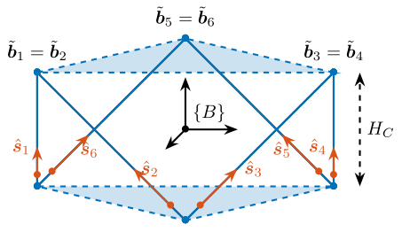

%% Analytical formula for Stiffness matrix of the Cubic Stewart platform
% Define symbolic variables
syms k Hc alpha H

assume(k > 0); % k is positive real
assume(Hc, 'real'); % Hc is real
assume(H, 'real'); % H is real
assume(alpha, 'real'); % alpha is real

% Define si matrix (edges of the cubes)
si = 1/sqrt(3)*[
  [ sqrt(2),    0,        1]; ...
  [-sqrt(2)/2, -sqrt(3/2), 1]; ...
  [-sqrt(2)/2,  sqrt(3/2), 1]; ...
  [ sqrt(2),    0,        1]; ...
  [-sqrt(2)/2, -sqrt(3/2), 1]; ...
  [-sqrt(2)/2,  sqrt(3/2), 1]  ...
];

% Define ci matrix (vertices of the cubes)
ci = Hc * [
  [1/sqrt(2), -sqrt(3)/sqrt(2), 0.5]; ...
  [1/sqrt(2), -sqrt(3)/sqrt(2), 0.5]; ...
  [1/sqrt(2),  sqrt(3)/sqrt(2), 0.5]; ...
  [1/sqrt(2),  sqrt(3)/sqrt(2), 0.5]; ...
  [-sqrt(2),   0,               0.5]; ...
  [-sqrt(2),   0,               0.5]  ...
];

% Apply vertical shift to ci
ci = ci + H * [0, 0, 1];

% Calculate bi vectors (Stewart platform top joints)
bi = ci + alpha * si;

% Initialize stiffness matrix
K = sym(zeros(6,6));

% Calculate elements of the stiffness matrix
for i = 1:6
    % Extract vectors for each leg
    s_i = si(i,:)';
    b_i = bi(i,:)';

    % Calculate cross product vector
    cross_bs = cross(b_i, s_i);

    % Build matrix blocks
    K(1:3, 4:6) = K(1:3, 4:6) + s_i * cross_bs';
    K(4:6, 1:3) = K(4:6, 1:3) + cross_bs * s_i';
    K(1:3, 1:3) = K(1:3, 1:3) + s_i * s_i';
    K(4:6, 4:6) = K(4:6, 4:6) + cross_bs * cross_bs';
end

% Scale by stiffness coefficient
K = k * K;

% Simplify the expressions
K = simplify(K);

% Display the analytical stiffness matrix
disp('Analytical Stiffness Matrix:');
pretty(K);

In that case (top joints at the cube's vertices), a diagonal stiffness matrix is obtained eqref:eq:detail_kinematics_cubic_stiffness. Translation stiffness is twice the stiffness of the struts, and rotational stiffness is proportional to the square of the cube's size Hc.

\begin{equation}\label{eq:detail_kinematics_cubic_stiffness} \bm{K}_{\{B\} = \{C\}} = k \begin{bmatrix} 2 & 0 & 0 & 0 & 0 & 0
0 & 2 & 0 & 0 & 0 & 0
0 & 0 & 2 & 0 & 0 & 0
0 & 0 & 0 & \frac{3}{2} H_c^2 & 0 & 0
0 & 0 & 0 & 0 & \frac{3}{2} H_c^2 & 0
0 & 0 & 0 & 0 & 0 & 6 H_c^2 \\

\end{bmatrix}

\end{equation}

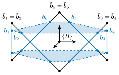
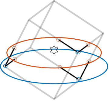
But typically, the top joints are not placed at the cube's vertices but on the cube's edges (Figure ref:fig:detail_kinematics_cubic_schematic). In that case, the location of the top joints can be expressed by eqref:eq:detail_kinematics_cubic_edges.

\begin{equation}\label{eq:detail_kinematics_cubic_edges} \bm{b}_i = ~{\bm{b}}_i + α \hat{\bm{s}}_i

\end{equation}

But the computed stiffness matrix is the same eqref:eq:detail_kinematics_cubic_stiffness.

The Stiffness matrix is diagonal for forces and torques applied on the top platform, but expressed at the center of the cube, and for translations and rotations of the top platform expressed with respect to the cube's center.

• Should I introduce the term "center of stiffness" here?

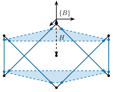
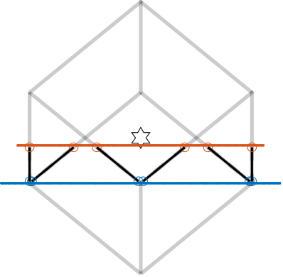
Effect of having frame $\{B\}$ off-centered

However, as soon as the location of the A and B frames are shifted from the cube's center, off diagonal elements in the stiffness matrix appear.

Let's consider here a vertical shift as shown in Figure ref:fig:detail_kinematics_cubic_schematic_off_centered. In that case, the stiffness matrix is eqref:eq:detail_kinematics_cubic_stiffness_off_centered. Off diagonal elements are increasing with the height difference between the cube's center and the considered B frame.

\begin{equation}\label{eq:detail_kinematics_cubic_stiffness_off_centered} \bm{K}_{\{B\} ≠ \{C\}} = k \begin{bmatrix} 2 & 0 & 0 & 0 & -2 H & 0
0 & 2 & 0 & 2 H & 0 & 0
0 & 0 & 2 & 0 & 0 & 0
0 & 2 H & 0 & \frac{3}{2} H_c^2 + 2 H^2 & 0 & 0
-2 H & 0 & 0 & 0 & \frac{3}{2} H_c^2 + 2 H^2 & 0
0 & 0 & 0 & 0 & 0 & 6 H_c^2 \\

\end{bmatrix}

\end{equation}

Such structure of the stiffness matrix is very typical with Stewart platform that have some symmetry, but not necessary only for cubic architectures.

Therefore, the stiffness of the cubic architecture is special only when considering a frame located at the center of the cube. This is not very convenient, as in the vast majority of cases, the interesting frame is located about the top platform.

Note that the cube's center needs not to be at the "center" of the Stewart platform. This can lead to interesting architectures shown in Section ref:ssec:detail_kinematics_cubic_design.

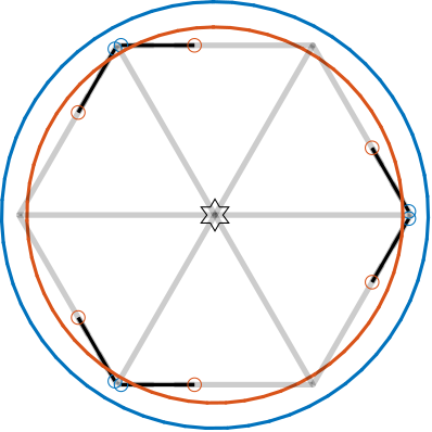
Uniform Mobility

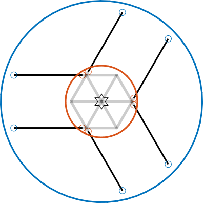
Uniform mobility in X,Y,Z directions (Figure ref:fig:detail_kinematics_cubic_mobility_translations)

• This is somehow more uniform than other architecture
• A cube is obtained
• The length of the cube's edge is equal to the strut axial stroke
• Mobility in translation does not depend on the cube's size

Some have argue that the translational mobility of the Cubic Stewart platform is a sphere cite:&mcinroy00_desig_contr_flexur_joint_hexap, and this is useful to be able to move equal amount in all directions. As shown here, this is wrong. It is possible the consider that the mobility is uniform along the directions of the struts, but usually these are not interesting directions.

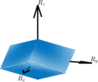
Also show mobility in Rx,Ry,Rz (Figure ref:fig:detail_kinematics_cubic_mobility_rotations):

• more mobility in Rx and Ry than in Rz
• Mobility decreases with the size of the cube

%% Cubic configuration
H = 100e-3;     % Height of the Stewart platform [m]
Hc = 100e-3;   % Size of the useful part of the cube [m]
FOc = 50e-3; % Center of the cube at the Stewart platform center
MO_B = -50e-3;  % Position {B} with respect to {M} [m]
MHb = 0;

stewart_cubic = initializeStewartPlatform();
stewart_cubic = initializeFramesPositions(stewart_cubic, 'H', H, 'MO_B', MO_B);
stewart_cubic = generateCubicConfiguration(stewart_cubic, 'Hc', Hc, 'FOc', FOc, 'FHa', 5e-3, 'MHb', MHb);
stewart_cubic = computeJointsPose(stewart_cubic);
stewart_cubic = initializeStrutDynamics(stewart_cubic, 'k', 1);
stewart_cubic = computeJacobian(stewart_cubic);
stewart_cubic = initializeCylindricalPlatforms(stewart_cubic, 'Fpr', 150e-3, 'Mpr', 150e-3);

% Let's now define the actuator stroke.
L_max =  50e-6; % [m]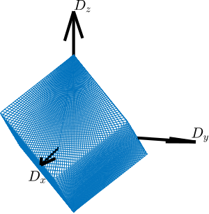

Dynamical Decoupling

<<ssec:detail_kinematics_cubic_dynamic>>

Introduction   ignore

• cite:&mcinroy00_desig_contr_flexur_joint_hexap Why is this here?

In this section, the dynamics of the platform in the cartesian frame is studied. This corresponds to the transfer function from forces and torques $\bm{\mathcal{F}}$ to translations and rotations $\bm{\mathcal{X}}$ of the top platform. If relative motion sensor are located in each strut ($\bm{\mathcal{L}}$ is measured), the pose $\bm{\mathcal{X}}$ is computed using the Jacobian matrix as shown in Figure ref:fig:detail_kinematics_centralized_control.

\begin{tikzpicture}
  \node[block] (Jt) at (0, 0) {$\bm{J}^{-T}$};
  \node[block, right= of Jt] (G) {$\bm{G}$};
  \node[block, right= of G] (J) {$\bm{J}^{-1}$};
  \node[block, left= of Jt] (Kx) {$\bm{K}_{\mathcal{X}}$};

  \draw[->] (Kx.east) -- node[midway, above]{$\bm{\mathcal{F}}$} (Jt.west);
  \draw[->] (Jt.east) -- (G.west) node[above left]{$\bm{\tau}$};
  \draw[->] (G.east) -- (J.west) node[above left]{$\bm{\mathcal{L}}$};
  \draw[->] (J.east) -- ++(1.0, 0);
  \draw[->] ($(J.east) + (0.5, 0)$)node[]{$\bullet$} node[above]{$\bm{\mathcal{X}}$} -- ++(0, -1) -| ($(Kx.west) + (-0.5, 0)$) -- (Kx.west);

  \begin{scope}[on background layer]
    \node[fit={(Jt.south west) (J.north east)}, fill=black!20!white, draw, dashed, inner sep=4pt] (Px) {};
    \node[anchor={south}] at (Px.north){\small{Cartesian Plant}};
  \end{scope}
\end{tikzpicture}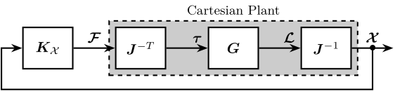

From Strut coordinate to Cartesian coordinate using the Jacobian matrix

We want to see if the Stewart platform has some special properties for control in the cartesian frame.

Low frequency and High frequency coupling

As was derived during the conceptual design phase, the dynamics from $\bm{\mathcal{F}}$ to $\bm{\mathcal{X}}$ is described by eqref:eq:detail_kinematics_transfer_function_cart

\begin{equation}\label{eq:detail_kinematics_transfer_function_cart} \frac{{\mathcal{X}}}{\bm{\mathcal{F}}}(s) = ( \bm{M} s^2 + \bm{J}^T \bm{\mathcal{C}} \bm{J} s + \bm{J}^T \bm{\mathcal{K}} \bm{J} )^-1

\end{equation}

At low frequency: the static behavior of the platform depends on the stiffness matrix eqref:eq:detail_kinematics_transfer_function_cart_low_freq.

\begin{equation}\label{eq:detail_kinematics_transfer_function_cart_low_freq} \frac{{\mathcal{X}}}{\bm{\mathcal{F}}}(j ω) \xrightarrow[ω → 0]{} \bm{K}^-1

\end{equation}

In section ref:ssec:detail_kinematics_cubic_static, it was shown that for the cubic configuration, the stiffness matrix is diagonal if frame $\{B\}$ is taken at the cube's center. In that case, the "cartesian" plant is decoupled at low frequency.

At high frequency, the behavior depends on the mass matrix (evaluated at frame B) eqref:eq:detail_kinematics_transfer_function_high_freq.

\begin{equation}\label{eq:detail_kinematics_transfer_function_high_freq} \frac{{\mathcal{X}}}{\bm{\mathcal{F}}}(j ω) \xrightarrow[ω → ∞]{} - ω^2 \bm{M}^-1

\end{equation}

To have the mass matrix diagonal, the center of mass of the mobile parts needs to coincide with the B frame and the principal axes of inertia of the body also needs to coincide with the axis of the B frame.

To verify that,

• CoM above the top platform (Figure ref:fig:detail_kinematics_cubic_payload)

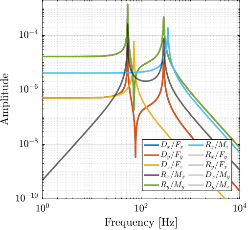
• The transfer functions from F to X are computed for two specific locations of the B frames:

  • center of mass: coupled at low frequency due to non diagonal stiffness matrix (Figure ref:fig:detail_kinematics_cubic_cart_coupling_com)
  • center of stiffness: coupled at high frequency due to non diagonal mass matrix (Figure ref:fig:detail_kinematics_cubic_cart_coupling_cok)
• In both cases, we would get similar dynamics for a non-cubic stewart platform.

%% Input/Output definition of the Simscape model
clear io; io_i = 1;
io(io_i) = linio([mdl, '/Controller'], 1, 'openinput');  io_i = io_i + 1; % Actuator Force Inputs [N]
io(io_i) = linio([mdl, '/plant'],      1, 'openoutput'); io_i = io_i + 1; % External metrology [m,rad]

% Prepare simulation
controller = initializeController('type', 'open-loop');
sample = initializeSample('type', 'cylindrical', 'm', 10, 'H', 100e-3, 'R', 100e-3);

%% Cubic Stewart platform with payload above the top platform - B frame at the CoM
H    = 200e-3; % height of the Stewart platform [m]
MO_B = 50e-3;  % Position {B} with respect to {M} [m]

stewart = initializeStewartPlatform();
stewart = initializeFramesPositions(stewart, 'H', H, 'MO_B', MO_B);
stewart = generateCubicConfiguration(stewart, 'Hc', H, 'FOc', H/2, 'FHa', 25e-3, 'MHb', 25e-3);
stewart = computeJointsPose(stewart);
stewart = initializeStrutDynamics(stewart, 'k', 1e6, 'c', 1e1);
stewart = initializeJointDynamics(stewart, 'type_F', '2dof', 'type_M', '3dof');
stewart = computeJacobian(stewart);
stewart = initializeStewartPose(stewart);
stewart = initializeCylindricalPlatforms(stewart, ...
                                         'Mpm', 1e-6, ... % Massless platform
                                         'Fpm', 1e-6, ... % Massless platform
                                         'Mph', 20e-3, ... % Thin platform
                                         'Fph', 20e-3, ... % Thin platform
                                         'Mpr', 1.2*max(vecnorm(stewart.platform_M.Mb)), ...
                                         'Fpr', 1.2*max(vecnorm(stewart.platform_F.Fa)));
stewart = initializeCylindricalStruts(stewart, ...
    'Fsm', 1e-6, ... % Massless strut
    'Msm', 1e-6, ... % Massless strut
    'Fsh', stewart.geometry.l(1)/2, ...
    'Msh', stewart.geometry.l(1)/2 ...
);

% Run the linearization
G_CoM = linearize(mdl, io)*inv(stewart.kinematics.J).';
G_CoM.InputName  = {'Fx', 'Fy', 'Fz', 'Mx', 'My', 'Mz'};
G_CoM.OutputName = {'Dx', 'Dy', 'Dz', 'Rx', 'Ry', 'Rz'};

%% Same geometry but B Frame at cube's center (CoK)
MO_B = -100e-3;  % Position {B} with respect to {M} [m]
stewart = initializeStewartPlatform();
stewart = initializeFramesPositions(stewart, 'H', H, 'MO_B', MO_B);
stewart = generateCubicConfiguration(stewart, 'Hc', H, 'FOc', H/2, 'FHa', 25e-3, 'MHb', 25e-3);
stewart = computeJointsPose(stewart);
stewart = initializeStrutDynamics(stewart, 'k', 1e6, 'c', 1e1);
stewart = initializeJointDynamics(stewart, 'type_F', '2dof', 'type_M', '3dof');
stewart = computeJacobian(stewart);
stewart = initializeStewartPose(stewart);
stewart = initializeCylindricalPlatforms(stewart, ...
                                         'Mpm', 1e-6, ... % Massless platform
                                         'Fpm', 1e-6, ... % Massless platform
                                         'Mph', 20e-3, ... % Thin platform
                                         'Fph', 20e-3, ... % Thin platform
                                         'Mpr', 1.2*max(vecnorm(stewart.platform_M.Mb)), ...
                                         'Fpr', 1.2*max(vecnorm(stewart.platform_F.Fa)));
stewart = initializeCylindricalStruts(stewart, ...
    'Fsm', 1e-6, ... % Massless strut
    'Msm', 1e-6, ... % Massless strut
    'Fsh', stewart.geometry.l(1)/2, ...
    'Msh', stewart.geometry.l(1)/2 ...
);

% Run the linearization
G_CoK = linearize(mdl, io)*inv(stewart.kinematics.J.');
G_CoK.InputName  = {'Fx', 'Fy', 'Fz', 'Mx', 'My', 'Mz'};
G_CoK.OutputName = {'Dx', 'Dy', 'Dz', 'Rx', 'Ry', 'Rz'};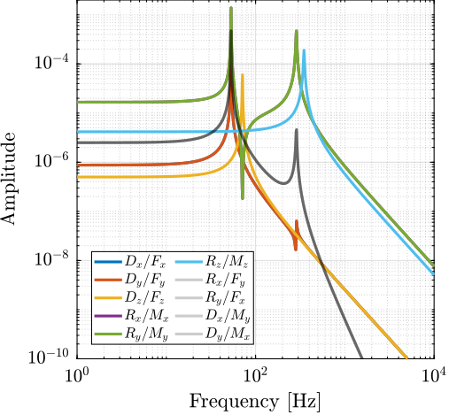

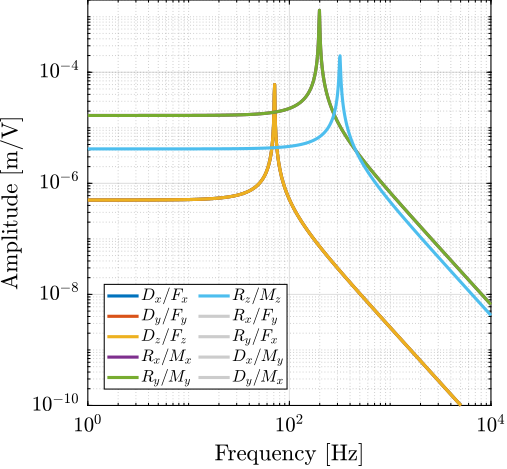
Payload's CoM at the cube's center

It is therefore natural to try to have the cube's center and the center of mass of the moving part coincide at the same location.

• CoM at the center of the cube: Figure ref:fig:detail_kinematics_cubic_centered_payload

This is what is physically done in cite:&mcinroy99_dynam;&mcinroy99_precis_fault_toler_point_using_stewar_platf;&mcinroy00_desig_contr_flexur_joint_hexap;&li01_simul_vibrat_isolat_point_contr;&jafari03_orthog_gough_stewar_platf_microm Shown in Figure ref:fig:detail_kinematics_uw_gsp

The obtained dynamics is indeed well decoupled, thanks to the diagonal stiffness matrix and mass matrix as the same time.

The main issue with this is that usually we want the payload to be located above the top platform, as it is the case for the nano-hexapod. Indeed, if a similar design than the one shown in Figure ref:fig:detail_kinematics_cubic_centered_payload was used, the x-ray beam will hit the different struts during the rotation of the spindle.

%% Cubic Stewart platform with payload above the top platform
H = 200e-3;
MO_B = -100e-3;  % Position {B} with respect to {M} [m]

stewart = initializeStewartPlatform();
stewart = initializeFramesPositions(stewart, 'H', H, 'MO_B', MO_B);
stewart = generateCubicConfiguration(stewart, 'Hc', H, 'FOc', H/2, 'FHa', 25e-3, 'MHb', 25e-3);
stewart = computeJointsPose(stewart);
stewart = initializeStrutDynamics(stewart, 'k', 1e6, 'c', 1e1);
stewart = initializeJointDynamics(stewart, 'type_F', '2dof', 'type_M', '3dof');
stewart = computeJacobian(stewart);
stewart = initializeStewartPose(stewart);
stewart = initializeCylindricalPlatforms(stewart, ...
                                         'Mpm', 1e-6, ... % Massless platform
                                         'Fpm', 1e-6, ... % Massless platform
                                         'Mph', 20e-3, ... % Thin platform
                                         'Fph', 20e-3, ... % Thin platform
                                         'Mpr', 1.2*max(vecnorm(stewart.platform_M.Mb)), ...
                                         'Fpr', 1.2*max(vecnorm(stewart.platform_F.Fa)));
stewart = initializeCylindricalStruts(stewart, ...
    'Fsm', 1e-6, ... % Massless strut
    'Msm', 1e-6, ... % Massless strut
    'Fsh', stewart.geometry.l(1)/2, ...
    'Msh', stewart.geometry.l(1)/2 ...
);

% Sample at the Center of the cube
sample = initializeSample('type', 'cylindrical', 'm', 10, 'H', 100e-3, 'H_offset', -H/2-50e-3);

% Run the linearization
G_CoM_CoK = linearize(mdl, io)*inv(stewart.kinematics.J.');
G_CoM_CoK.InputName  = {'Fx', 'Fy', 'Fz', 'Mx', 'My', 'Mz'};
G_CoM_CoK.OutputName = {'Dx', 'Dy', 'Dz', 'Rx', 'Ry', 'Rz'};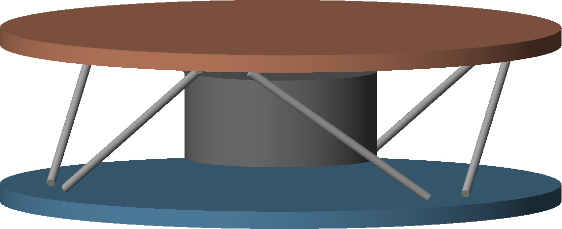

Conclusion

• Some work to still be decoupled when considering flexible joint stiffness

  • Find the reference
• Better decoupling between the struts? Next section

Some conclusions can be drawn from the above analysis:

• Static Decoupling <=> Diagonal Stiffness matrix <=> {A} and {B} at the cube's center
• Dynamic Decoupling <=> Static Decoupling + CoM of mobile platform coincident with {A} and {B}.
• Not specific to the cubic architecture
• Same stiffness in XYZ => Possible to have dynamic isotropy

Decentralized Control

<<ssec:detail_kinematics_decentralized_control>>

Introduction   ignore

From cite:preumont07_six_axis_singl_stage_activ, the cubic configuration "minimizes the cross-coupling amongst actuators and sensors of different legs (being orthogonal to each other)". This would facilitate the use of decentralized control.

\begin{tikzpicture}
  \node[block] (G) at (0,0) {$\bm{G}$};

  \node[block, left= of G] (Kl) {$\bm{K}_{\mathcal{L}}$};

  \draw[->] (Kl.east) -- node[midway, above]{$\bm{\tau}$} (G.west);
  \draw[->] (G.east) -- ++(1.0, 0);
  \draw[->] ($(G.east) + (0.5, 0)$)node[]{$\bullet$} node[above]{$\bm{\mathcal{L}}$} -- ++(0, -1) -| ($(Kl.west) + (-0.5, 0)$) -- (Kl.west);

  \begin{scope}[on background layer]
    \node[fit={(G.south west) (G.north east)}, fill=black!20!white, draw, dashed, inner sep=4pt] (Pl) {};
    \node[anchor={south}] at (Pl.north){\small{Strut Plant}};
  \end{scope}
\end{tikzpicture}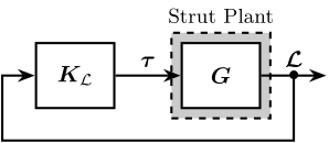

From Strut coordinate to Cartesian coordinate using the Jacobian matrix

In this section, we wish to study such properties of the cubic architecture.

Here, the plant output are sensors integrated in the Stewart platform struts. Two sensors are considered: a displacement sensor and a force sensor.

We will compare the transfer function from sensors to actuators in each strut for a cubic architecture and for a non-cubic architecture (where the struts are not orthogonal with each other).

The "strut plant" are compared for two Stewart platforms:

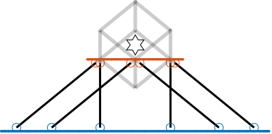
• with cubic architecture shown in Figure ref:fig:detail_kinematics_cubic_payload (page pageref:fig:detail_kinematics_cubic_payload)
• with a Stewart platform shown in Figure ref:fig:detail_kinematics_non_cubic_payload. It has the same payload and strut dynamics than for the cubic architecture. The struts are oriented more vertically to be far away from the cubic architecture

%% Input/Output definition of the Simscape model
clear io; io_i = 1;
io(io_i) = linio([mdl, '/Controller'], 1, 'openinput');  io_i = io_i + 1; % Actuator Force Inputs [N]
io(io_i) = linio([mdl, '/plant'],      2, 'openoutput', [], 'dL'); io_i = io_i + 1; % Displacement sensors [m]
io(io_i) = linio([mdl, '/plant'],      2, 'openoutput', [], 'fn'); io_i = io_i + 1; % Force Sensor [N]

% Prepare simulation : Payload above the top platform
controller = initializeController('type', 'open-loop');
sample = initializeSample('type', 'cylindrical', 'm', 10, 'H', 100e-3, 'R', 100e-3);

%% Cubic Stewart platform
H    = 200e-3; % height of the Stewart platform [m]
MO_B = 50e-3;  % Position {B} with respect to {M} [m]

stewart = initializeStewartPlatform();
stewart = initializeFramesPositions(stewart, 'H', H, 'MO_B', MO_B);
stewart = generateCubicConfiguration(stewart, 'Hc', H, 'FOc', H/2, 'FHa', 25e-3, 'MHb', 25e-3);
stewart = computeJointsPose(stewart);
stewart = initializeStrutDynamics(stewart, 'k', 1e6, 'c', 1e1);
stewart = initializeJointDynamics(stewart, 'type_F', '2dof', 'type_M', '3dof');
stewart = computeJacobian(stewart);
stewart = initializeStewartPose(stewart);
stewart = initializeCylindricalPlatforms(stewart, ...
                                         'Mpm', 1e-6, ... % Massless platform
                                         'Fpm', 1e-6, ... % Massless platform
                                         'Mph', 20e-3, ... % Thin platform
                                         'Fph', 20e-3, ... % Thin platform
                                         'Mpr', 1.2*max(vecnorm(stewart.platform_M.Mb)), ...
                                         'Fpr', 1.2*max(vecnorm(stewart.platform_F.Fa)));
stewart = initializeCylindricalStruts(stewart, ...
    'Fsm', 1e-6, ... % Massless strut
    'Msm', 1e-6, ... % Massless strut
    'Fsh', stewart.geometry.l(1)/2, ...
    'Msh', stewart.geometry.l(1)/2 ...
);

% Run the linearization
G_cubic = linearize(mdl, io);
G_cubic.InputName  = {'f1', 'f2', 'f3', 'f4', 'f5', 'f6'};
G_cubic.OutputName = {'dL1', 'dL2', 'dL3', 'dL4', 'dL5', 'dL6', ...
                      'fn1', 'fn2', 'fn3', 'fn4', 'fn5', 'fn6'};

%% Non-Cubic Stewart platform
stewart = initializeStewartPlatform();
stewart = initializeFramesPositions(stewart, 'H', H, 'MO_B', MO_B);
stewart = generateCubicConfiguration(stewart, 'Hc', H, 'FOc', H/2, 'FHa', 25e-3, 'MHb', 25e-3);
stewart = generateGeneralConfiguration(stewart, 'FH', 25e-3, 'FR', 250e-3, 'MH', 25e-3, 'MR', 250e-3, ...
                                      'FTh', [-22, 22, 120-22, 120+22, 240-22, 240+22]*(pi/180), ...
                                      'MTh', [-60+22, 60-22, 60+22, 180-22, 180+22, -60-22]*(pi/180));
stewart = computeJointsPose(stewart);
stewart = initializeStrutDynamics(stewart, 'k', 1e6, 'c', 1e1);
stewart = initializeJointDynamics(stewart, 'type_F', '2dof', 'type_M', '3dof');
stewart = computeJacobian(stewart);
stewart = initializeStewartPose(stewart);
stewart = initializeCylindricalPlatforms(stewart, ...
                                         'Mpm', 1e-6, ... % Massless platform
                                         'Fpm', 1e-6, ... % Massless platform
                                         'Mph', 20e-3, ... % Thin platform
                                         'Fph', 20e-3, ... % Thin platform
                                         'Mpr', 1.2*max(vecnorm(stewart.platform_M.Mb)), ...
                                         'Fpr', 1.2*max(vecnorm(stewart.platform_F.Fa)));
stewart = initializeCylindricalStruts(stewart, ...
    'Fsm', 1e-6, ... % Massless strut
    'Msm', 1e-6, ... % Massless strut
    'Fsh', stewart.geometry.l(1)/2, ...
    'Msh', stewart.geometry.l(1)/2 ...
);

% Run the linearization
G_non_cubic = linearize(mdl, io);
G_non_cubic.InputName  = {'f1', 'f2', 'f3', 'f4', 'f5', 'f6'};
G_non_cubic.OutputName = {'dL1', 'dL2', 'dL3', 'dL4', 'dL5', 'dL6', ...
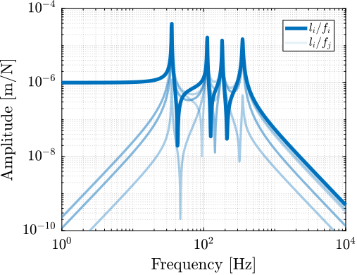
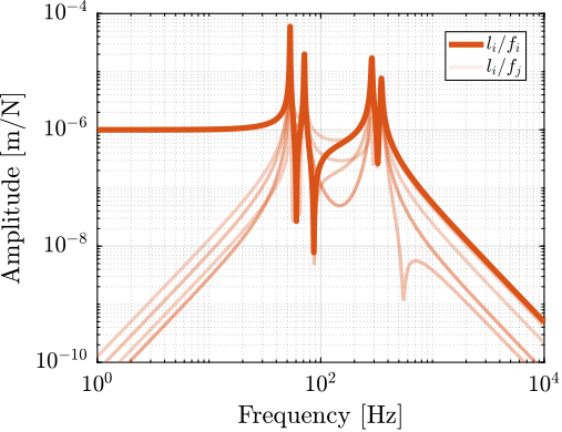
                          'fn1', 'fn2', 'fn3', 'fn4', 'fn5', 'fn6'};

Relative Displacement Sensors

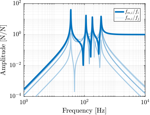
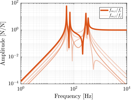
The transfer functions from actuator force included in each strut to the relative motion of the struts are shown in Figure ref:fig:detail_kinematics_decentralized_dL. As expected from the equations of motion from $\bm{f}$ to $\bm{\mathcal{L}}$ eqref:eq:nhexa_transfer_function_struts, the $6 \times 6$ plants are decoupled at low frequency.

At high frequency, the plant is coupled as the mass matrix projected in the frame of the struts is not diagonal.

No clear advantage can be seen for the cubic architecture (figure ref:fig:detail_kinematics_cubic_decentralized_dL) as compared to the non-cubic architecture (Figure ref:fig:detail_kinematics_non_cubic_decentralized_dL).

Note that the resonance frequencies are not the same in both cases as having the struts oriented more vertically changed the stiffness properties of the Stewart platform and hence the frequency of different modes.

Force Sensors

Similarly, the transfer functions from actuator force to force sensors included in each strut are extracted both for the cubic and non-cubic Stewart platforms.

The results are shown in Figure ref:fig:detail_kinematics_decentralized_fn.

Conclusion

The Cubic architecture seems to not have any significant effect on the coupling between actuator and sensors of each strut and thus provides no advantages for decentralized control.

Cubic architecture with Cube's center above the top platform

<<ssec:detail_kinematics_cubic_design>>

Introduction   ignore

As was shown in Section ref:ssec:detail_kinematics_cubic_dynamic, the cubic architecture can have very interesting dynamical properties when the center of mass of the moving body is at the cube's center.

This is because, both the mass and stiffness matrices are diagonal. As shown in in section ref:ssec:detail_kinematics_cubic_static, the stiffness matrix is diagonal when the considered B frame is located at the cube's center.

Or, typically the $\{B\}$ frame is taken above the top platform where forces are applied and where displacements are expressed.

In this section, modifications of the Cubic architectures are proposed in order to be able to have the payload above the top platform while still benefiting from interesting dynamical properties of the cubic architecture.

There are three key parameters:

• $H$ height of the Stewart platform (distance from fix base to mobile platform)
• $H_c$ height of the cube, as shown in Figure ref:fig:detail_kinematics_cubic_schematic_full
• $H_{CoM}$ height of the center of mass with respect to the mobile platform. It is also the cube's center.

The obtained design depends on the considered size of the cube $H_c$ with respect to $H$ and $H_{CoM}$.

%% Cubic configurations with center of the cube above the top platform
H    = 100e-3; % height of the Stewart platform [m]
MO_B = 20e-3;  % Position {B} with respect to {M} [m]
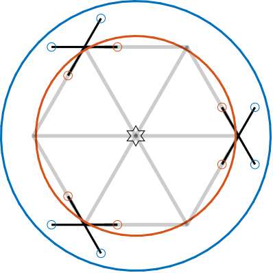
FOc  = H + MO_B; % Center of the cube with respect to {F}

Small cube

When the considered cube size is smaller than twice the height of the CoM, the obtained design looks like Figure ref:fig:detail_kinematics_cubic_above_small.

\begin{equation}\label{eq:detail_kinematics_cube_small} H_c < 2 H_CoM

\end{equation}

This is similar to cite:&furutani04_nanom_cuttin_machin_using_stewar, even though it is not mentioned that the system has a cubic configuration.

Adjacent struts are parallel to each other, which is quite different from the typical architecture in which parallel struts are opposite to each other.

%% Small cube
Hc   = 2*MO_B;    % Size of the useful part of the cube [m]

stewart_small = initializeStewartPlatform();
stewart_small = initializeFramesPositions(stewart_small, 'H', H, 'MO_B', MO_B);
stewart_small = generateCubicConfiguration(stewart_small, 'Hc', Hc, 'FOc', FOc, 'FHa', 5e-3, 'MHb', 5e-3);
stewart_small = computeJointsPose(stewart_small);
stewart_small = initializeStrutDynamics(stewart_small, 'k', 1);
stewart_small = computeJacobian(stewart_small);
stewart_small = initializeCylindricalPlatforms(stewart_small, 'Fpr', 1.1*max(vecnorm(stewart_small.platform_F.Fa)), 'Mpr', 1.1*max(vecnorm(stewart_small.platform_M.Mb)));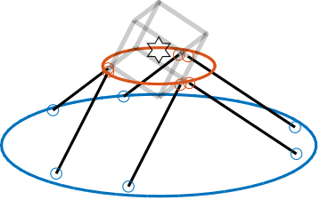

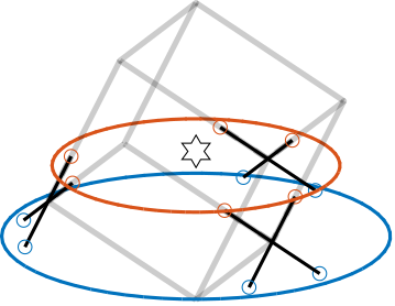
Medium sized cube

Increasing the cube size with an height close to the stewart platform height leads to an architecture in which the struts are crossing.

\begin{equation}\label{eq:detail_kinematics_cube_medium} 2 H_CoM < H_c < 2 (H_CoM + H)

\end{equation}

This is similar to cite:yang19_dynam_model_decoup_contr_flexib (Figure ref:fig:detail_kinematics_yang19 in page pageref:fig:detail_kinematics_yang19), even though it is not cubic (but the struts are crossing).

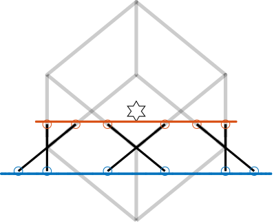
Large cube

When the cube's height is more than twice the platform height added to the CoM height, the architecture shown in Figure ref:fig:detail_kinematics_cubic_above_large is obtained.

\begin{equation}\label{eq:detail_kinematics_cube_large} 2 (H_CoM + H) < H_c

\end{equation}

Platform size

%% Get the analytical formula for the location of the top and bottom joints
% Define symbolic variables
syms k Hc Hcom alpha H

assume(k > 0); % k is positive real
assume(Hcom > 0); % k is positive real
assume(Hc > 0); % Hc is real
assume(H > 0); % H is real
assume(alpha, 'real'); % alpha is real

% Define si matrix (edges of the cubes)
si = 1/sqrt(3)*[
  [ sqrt(2),    0,        1]; ...
  [-sqrt(2)/2, -sqrt(3/2), 1]; ...
  [-sqrt(2)/2,  sqrt(3/2), 1]; ...
  [ sqrt(2),    0,        1]; ...
  [-sqrt(2)/2, -sqrt(3/2), 1]; ...
  [-sqrt(2)/2,  sqrt(3/2), 1]  ...
];

% Define ci matrix (vertices of the cubes)
ci = Hc * [
  [1/sqrt(2), -sqrt(3)/sqrt(2), 0.5]; ...
  [1/sqrt(2), -sqrt(3)/sqrt(2), 0.5]; ...
  [1/sqrt(2),  sqrt(3)/sqrt(2), 0.5]; ...
  [1/sqrt(2),  sqrt(3)/sqrt(2), 0.5]; ...
  [-sqrt(2),   0,               0.5]; ...
  [-sqrt(2),   0,               0.5]  ...
];

% Apply vertical shift to ci
ci = ci + (H + Hcom) * [0, 0, 1];

% Calculate bi vectors (Stewart platform top joints)
bi = ci + alpha * si;


% Extract the z-component value from the first row of ci
% (all rows have the same z-component)
ci_z = ci(1, 3);

% The z-component of si is 1 for all rows
si_z = si(1, 3);

alpha_for_0 = solve(ci_z + alpha * si_z == 0, alpha);
alpha_for_H = solve(ci_z + alpha * si_z == H, alpha);

% Verify the results
% Substitute alpha values and check the resulting bi_z values
bi_z_0 = ci + alpha_for_0 * si;
disp('Verification bi_z = 0:');
disp(simplify(bi_z_0));

bi_z_H = ci + alpha_for_H * si;
disp('Verification bi_z = H:');
disp(simplify(bi_z_H));

% Compute radius
simplify(sqrt(bi_z_H(:,1).^2 + bi_z_H(:,2).^2))
simplify(sqrt(bi_z_0(:,1).^2 + bi_z_0(:,2).^2))

The top joints $\bm{b}_i$ are located on a circle with radius $R_{b_i}$ eqref:eq:detail_kinematics_cube_top_joints. The bottom joints $\bm{a}_i$ are located on a circle with radius $R_{a_i}$ eqref:eq:detail_kinematics_cube_bot_joints.

\begin{subequations}\label{eq:detail_kinematics_cube_joints}

\begin{align} R_{b_i} &= \sqrt{\frac{3}{2} H_c^2 + 2 H_{CoM}^2} \label{eq:detail_kinematics_cube_top_joints} \\ R_{a_i} &= \sqrt{\frac{3}{2} H_c^2 + 2 (H_{CoM} + H)^2} \label{eq:detail_kinematics_cube_bot_joints} \end{align}

\end{subequations}

The size of the platforms increase with the cube's size and the height of the location of the center of mass (also coincident with the cube's center). The size of the bottom platform also increases with the height of the Stewart platform.

As the rotational stiffness for the cubic architecture is scaled as the square of the cube's height eqref:eq:detail_kinematics_cubic_stiffness, the cube's size can be determined from the requirements in terms of rotational stiffness. Then, using eqref:eq:detail_kinematics_cube_joints, the size of the top and bottom platforms can be determined.

Conclusion

For each of the configuration, the Stiffness matrix is diagonal with $k_x = k_y = k_y = 2k$ with $k$ is the stiffness of each strut. However, the rotational stiffnesses are increasing with the cube's size but the required size of the platform is also increasing, so there is a trade-off here.

We found that we can have a diagonal stiffness matrix using the cubic architecture when $\{A\}$ and $\{B\}$ are located above the top platform. Depending on the cube's size, we obtain 3 different configurations.

Conclusion

Cubic architecture can be interesting when specific payloads are being used. In that case, the center of mass of the payload should be placed at the center of the cube. For the classical architecture, it is often not possible.

Architectures with the center of the cube about the top platform are proposed to overcome this issue.

Cubic architecture are attributed a number of properties that were found to be incorrect:

• Uniform mobility
• Easy for decentralized control

Nano Hexapod

<<sec:detail_kinematics_nano_hexapod>>

Introduction   ignore

For the NASS, the chosen frame $\{A\}$ and $\{B\}$ coincide with the sample's point of interest, which is $150\,mm$ above the top platform.

Requirements:

• The nano-hexapod should fit within a cylinder with radius of $120\,mm$ and with a height of $95\,mm$.
• In terms of mobility: uniform mobility in XYZ directions (100um)
• In terms of stiffness: ?? Having the resonance frequencies well above the maximum rotational velocity of $2\pi\,\text{rad/s}$ to limit the gyroscopic effects. Having the resonance below the problematic modes of the micro-station to decouple from the micro-station complex dynamics.

• In terms of dynamics:

  • be able to apply IFF in a decentralized way with good robustness and performances (good damping of modes)
  • good decoupling for the HAC

The main difficulty for the design optimization of the nano-hexapod, is that the payloads will have various inertia, with masses ranging from 1 to 50kg. It is therefore not possible to have one geometry that gives good dynamical properties for all the payloads.

It could have been an option to have a cubic architecture as proposed in section ref:ssec:detail_kinematics_cubic_design, but having the cube's center 150mm above the top platform would have lead to platforms well exceeding the maximum available size. In that case, each payload would have to be calibrated in inertia before placing on top of the nano-hexapod, which would require a lot of work from the future users.

Considering the fact that it would not be possible to have the center of mass at the cube's center, the cubic architecture is not of great value here.

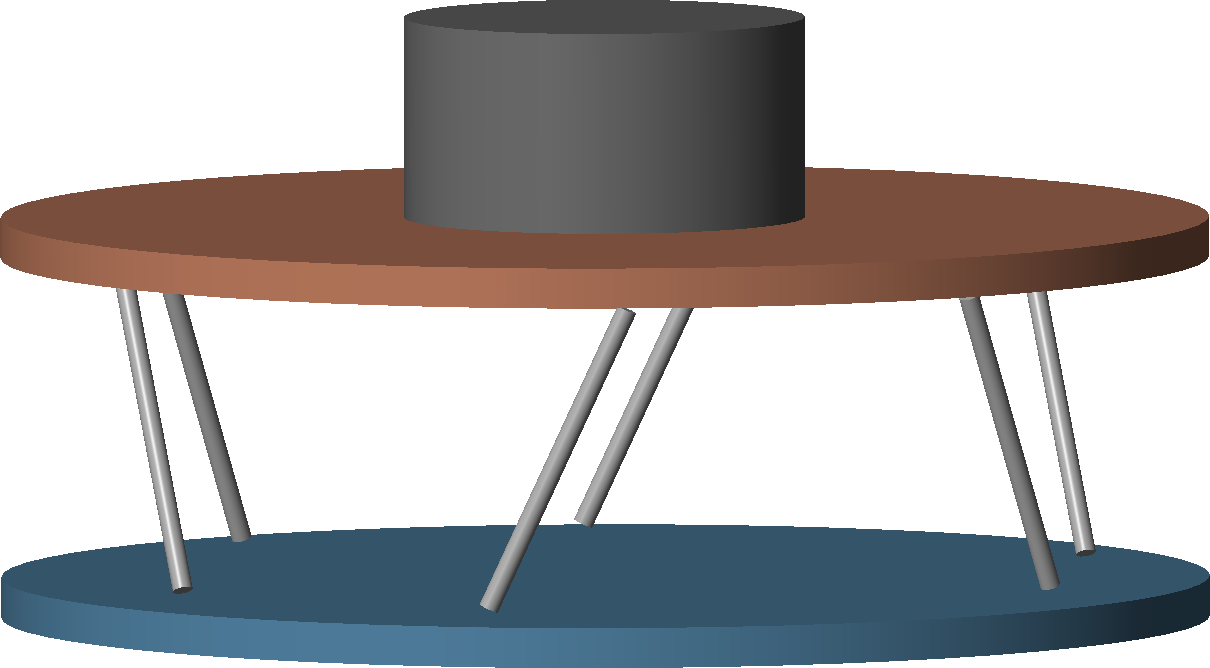
Obtained Geometry

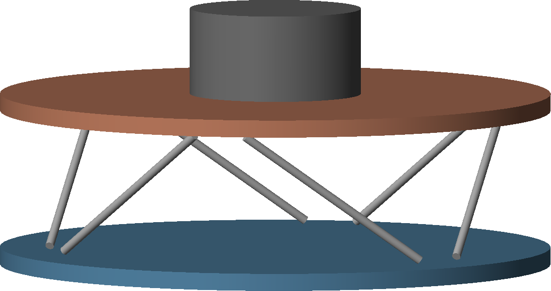
Take both platforms at maximum size. Make reasonable choice (close to the final choice). Say that it is good enough to make all the calculations. The geometry will be slightly refined during the detailed mechanical design for several reason: easy of mount, manufacturability, …

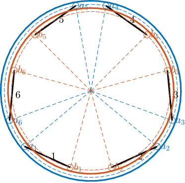
Obtained geometry is shown in Figure ref:fig:detail_kinematics_nano_hexapod. Height between the top plates is 95mm. Joints are offset by 15mm from the plate surfaces, and are positioned along a circle with radius 120mm for the fixed joints and 110mm for the mobile joints. The positioning angles (Figure ref:fig:detail_kinematics_nano_hexapod_top) are $[255, 285, 15, 45, 135, 165]$ degrees for the top joints and $[220, 320, 340, 80, 100, 200]$ degrees for the bottom joints.

%% Obtained Nano Hexapod Design
nano_hexapod = initializeStewartPlatform();
nano_hexapod = initializeFramesPositions(nano_hexapod, ...
                                    'H', 95e-3, ...
                                    'MO_B', 150e-3);

nano_hexapod = generateGeneralConfiguration(nano_hexapod, ...
                                       'FH', 15e-3, ...
                                       'FR', 120e-3, ...
                                       'FTh', [220, 320, 340, 80, 100, 200]*(pi/180), ...
                                       'MH', 15e-3, ...
                                       'MR', 110e-3, ...
                                       'MTh', [255, 285, 15, 45, 135, 165]*(pi/180));
nano_hexapod = computeJointsPose(nano_hexapod);
nano_hexapod = initializeStrutDynamics(nano_hexapod, 'k', 1);
nano_hexapod = computeJacobian(nano_hexapod);
nano_hexapod = initializeCylindricalPlatforms(nano_hexapod, 'Fpr', 125e-3, 'Mpr', 115e-3);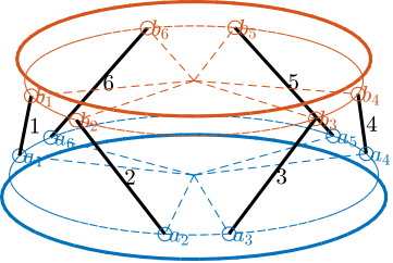

This geometry will be used for:

• estimate required actuator stroke
• estimate flexible joint stroke
• when performing noise budgeting for the choice of instrumentation
• for control purposes

It is only when the complete mechanical design is finished (Section …), that the model will be updated.

Required Actuator stroke

The actuator stroke to have the wanted mobility is computed.

Wanted mobility:

• Combined translations in the xyz directions of +/-50um (basically "cube")
• At any point of the cube, be able to do combined Rx and Ry rotations of +/-50urad
• Rz is always at 0
• Say that it is frame B with respect to frame A, but it is motion expressed at the point of interest (at the focus point of the light)

First the minimum actuator stroke to have the wanted mobility is computed. With the chosen geometry, an actuator stroke of +/-94um is found.

max_translation = 50e-6;
max_rotation = 50e-6;

Dxs = linspace(-max_translation, max_translation, 3);
Dys = linspace(-max_translation, max_translation, 3);
Dzs = linspace(-max_translation, max_translation, 3);
Rxs = linspace(-max_rotation, max_rotation, 3);
Rys = linspace(-max_rotation, max_rotation, 3);

L_min = 0;
L_max = 0;

for Dx = Dxs
for Dy = Dys
for Dz = Dzs
for Rx = Rxs
for Ry = Rys
    ARB = [ cos(Ry) 0        sin(Ry);
            0       1        0;
           -sin(Ry) 0        cos(Ry)] * ...
          [ 1       0        0;
            0       cos(Rx) -sin(Rx);
            0       sin(Rx)  cos(Rx)];

    [~, Ls] = inverseKinematics(nano_hexapod, 'AP', [Dx;Dy;Dz], 'ARB', ARB);

    if min(Ls) < L_min
        L_min = min(Ls);
    end
    if max(Ls) > L_max
        L_max = max(Ls);
    end
end
end
end
end
end

sprintf('Actuator stroke should be from %.0f um to %.0f um', 1e6*L_min, 1e6*L_max)

Considering combined rotations and translations, the wanted mobility and the obtained mobility of the Nano hexapod are shown in Figure …

It can be seen that just wanted mobility (displayed as a cube), just fits inside the obtained mobility. Here the worst case scenario is considered, meaning that whatever the angular position in Rx and Ry (in the range +/-50urad), the top platform can be positioned anywhere inside the cube.

%% Compute mobility in translation with combined angular motion
% L_max = 100e-6; % Actuator Stroke (+/-)

% Direction of motion (spherical coordinates)
thetas = linspace(0, pi, 100);
phis = linspace(0, 2*pi, 100);

% Considered Rotations
Rxs = linspace(-max_rotation, max_rotation, 3);
Rys = linspace(-max_rotation, max_rotation, 3);

% Maximum distance that can be reached in the direction of motion
% Considering combined angular motion and limited actuator stroke
rs = zeros(length(thetas), length(phis));
worst_rx_ry = zeros(length(thetas), length(phis), 2);

for i = 1:length(thetas)
    for j = 1:length(phis)
        % Compute unitary motion in the considered direction
        Tx = sin(thetas(i))*cos(phis(j));
        Ty = sin(thetas(i))*sin(phis(j));
        Tz = cos(thetas(i));
        % Start without considering rotations
        dL_lin = nano_hexapod.kinematics.J*[Tx; Ty; Tz; 0; 0; 0];
        % Strut motion for maximum displacement in the considered direction
        dL_lin_max = L_max*dL_lin/max(abs(dL_lin));

        % Find rotation that gives worst case stroke
        dL_worst = max(abs(dL_lin_max)); % This should be equal to L_max
        dL_rot_max = zeros(6,1);
        % Perform (small) rotations, and find the (worst) case requiring maximum strut motion
        for Rx = Rxs
        for Ry = Rys
                dL_rot = nano_hexapod.kinematics.J*[0; 0; 0; Rx; Ry; 0];
                if max(abs(dL_lin_max + dL_rot)) > dL_worst
                    dL_worst = max(abs(dL_lin_max + dL_rot));
                    dL_rot_max = dL_rot;
                    worst_rx_ry(i,j,:) = [Rx, Ry];
                end
        end
        end

        stroke_ratio = min(abs([( L_max - dL_rot_max) ./ dL_lin_max; (-L_max - dL_rot_max) ./ dL_lin_max]));
        dL_real = dL_lin_max*stroke_ratio + dL_rot_max;

        % % Obtained maximum displacement in the considered direction with angular motion
        % rs(i, j) = stroke_ratio*max(abs(dL_lin_max));
        rs(i, j) = stroke_ratio*L_max/max(abs(dL_lin));
    end
end

min(min(rs))
max(max(rs))

[phi_grid, theta_grid] = meshgrid(phis, thetas);
X = 1e6 * rs .* sin(theta_grid) .* cos(phi_grid);
Y = 1e6 * rs .* sin(theta_grid) .* sin(phi_grid);
Z = 1e6 * rs .* cos(theta_grid);

vertices = 1e6*max_translation*[
    -1 -1 -1;  % vertex 1
     1 -1 -1;  % vertex 2
     1  1 -1;  % vertex 3
    -1  1 -1;  % vertex 4
    -1 -1  1;  % vertex 5
     1 -1  1;  % vertex 6
     1  1  1;  % vertex 7
    -1  1  1   % vertex 8
];

% Define the faces using the vertex indices
faces = [
    1 2 3 4;  % bottom face
    5 6 7 8;  % top face
    1 2 6 5;  % front face
    2 3 7 6;  % right face
    3 4 8 7;  % back face
    4 1 5 8   % left face
];

figure;
hold on;
s = surf(X, Y, Z, 'FaceColor', 'none');
s.EdgeColor = colors(2, :);
patch('Vertices', vertices, 'Faces', faces, ...
      'FaceColor', [0.7 0.7 0.7], ...
      'EdgeColor', 'black', ...
      'FaceAlpha', 1);
hold off;
axis equal;
grid on;
xlabel('X Translation [$\mu$m]'); ylabel('Y Translation [$\mu$m]'); zlabel('Z Translation [$\mu$m]');
xlim(2e6*[-L_max, L_max]); ylim(2e6*[-L_max, L_max]); zlim(2e6*[-L_max, L_max]);

Therefore, in Section …, the specification for actuator stroke is +/-100um

Required Joint angular stroke

Now that the mobility of the Stewart platform is know, the corresponding flexible joint stroke can be estimated.

• conclude on the required joint angle: 1mrad? Will be used to design flexible joints.

%% Estimation of the required flexible joint angular stroke
max_angles = zeros(1,6);

% Compute initial strut orientation
nano_hexapod = computeJointsPose(nano_hexapod, 'AP', zeros(3,1), 'ARB', eye(3));
As = nano_hexapod.geometry.As;

% Only consider translations, but add maximum expected top platform rotation
for i = 1:length(thetas)
    for j = 1:length(phis)
        % Maximum translations
        Tx = rs(i,j)*sin(thetas(i))*cos(phis(j));
        Ty = rs(i,j)*sin(thetas(i))*sin(phis(j));
        Tz = rs(i,j)*cos(thetas(i));

        nano_hexapod = computeJointsPose(nano_hexapod, 'AP', [Tx; Ty; Tz], 'ARB', eye(3));

        angles = acos(dot(As, nano_hexapod.geometry.As));
        larger_angles = abs(angles) > max_angles;
        max_angles(larger_angles) = angles(larger_angles);
    end
end

sprintf('Maximum flexible joint angle is %.1f mrad', 1e3*max(max_angles))

Conclusion

<<sec:detail_kinematics_conclusion>>

Inertia used for experiments will be very broad => difficult to optimize the dynamics Specific geometry is not found to have a huge impact on performances. Practical implementation is important.

Geometry impacts the static and dynamical characteristics of the Stewart platform. Considering the design constrains, the slight change of geometry will not significantly impact the obtained results.

Bibliography   ignore