phd-nass-fem/index.org

Finite Element Model with Simscape

• Amplified Piezoelectric Actuator - 3D elements
  • Introduction
  • Import Mass Matrix, Stiffness Matrix, and Interface Nodes Coordinates
  • Output parameters
  • Piezoelectric parameters
  • Identification of the Dynamics
  • Comparison with Ansys
  • Force Sensor
  • Distributed Actuator
  • Distributed Actuator and Force Sensor
  • Dynamics from input voltage to displacement
  • Dynamics from input voltage to output voltage
• APA300ML
  • Introduction
  • Import Mass Matrix, Stiffness Matrix, and Interface Nodes Coordinates
  • Output parameters
  • Piezoelectric parameters
  • Identification of the APA Characteristics
    • Stiffness
    • Resonance Frequency
    • Amplification factor
    • Stroke
  • Identification of the Dynamics
  • IFF
  • DVF
  • Identification for a simpler model
• Flexible Joint
  • Introduction
  • Import Mass Matrix, Stiffness Matrix, and Interface Nodes Coordinates
  • Output parameters
  • Flexible Joint Characteristics
  • Identification of the parameters using Simscape
  • Simpler Model
• Integral Force Feedback with Amplified Piezo
  • Introduction
  • Import Mass Matrix, Stiffness Matrix, and Interface Nodes Coordinates
  • IFF Plant
  • IFF controller
  • Closed Loop System
• Bibliography

Amplified Piezoelectric Actuator - 3D elements

Introduction   ignore

The idea here is to:

• export a FEM of an amplified piezoelectric actuator from Ansys to Matlab
• import it into a Simscape model
• compare the obtained dynamics
• add 10kg mass on top of the actuator and identify the dynamics
• compare with results from Ansys where 10kg are directly added to the FEM

Import Mass Matrix, Stiffness Matrix, and Interface Nodes Coordinates

We first extract the stiffness and mass matrices.

  K = extractMatrix('piezo_amplified_3d_K.txt');
  M = extractMatrix('piezo_amplified_3d_M.txt');

Then, we extract the coordinates of the interface nodes.

  [int_xyz, int_i, n_xyz, n_i, nodes] = extractNodes('piezo_amplified_3d.txt');

  save('./mat/piezo_amplified_3d.mat', 'int_xyz', 'int_i', 'n_xyz', 'n_i', 'nodes', 'M', 'K');

Output parameters

  load('./mat/piezo_amplified_3d.mat', 'int_xyz', 'int_i', 'n_xyz', 'n_i', 'nodes', 'M', 'K');

Total number of Nodes	168959
Number of interface Nodes	13
Number of Modes	30
Size of M and K matrices	108

Interface Nodes for the Amplified Piezo Actuator

Node i	Node Number	x [m]	y [m]	z [m]
1.0	168947.0	0.0	0.03	0.0
2.0	168949.0	0.0	-0.03	0.0
3.0	168950.0	-0.035	0.0	0.0
4.0	168951.0	-0.028	0.0	0.0
5.0	168952.0	-0.021	0.0	0.0
6.0	168953.0	-0.014	0.0	0.0
7.0	168954.0	-0.007	0.0	0.0
8.0	168955.0	0.0	0.0	0.0
9.0	168956.0	0.007	0.0	0.0
10.0	168957.0	0.014	0.0	0.0
11.0	168958.0	0.021	0.0	0.0
12.0	168959.0	0.035	0.0	0.0
13.0	168960.0	0.028	0.0	0.0

Coordinates of the interface nodes

300000000.0	-30000.0	8000.0	-200.0	-30.0	-60000.0	20000000.0	-4000.0	500.0	8
-30000.0	100000000.0	400.0	30.0	200.0	-1	4000.0	-8000000.0	800.0	7
8000.0	400.0	50000000.0	-800000.0	-300.0	-40.0	300.0	100.0	5000000.0	40000.0
-200.0	30.0	-800000.0	20000.0	5	1	-10.0	-2	-40000.0	-300.0
-30.0	200.0	-300.0	5	40000.0	0.3	-4	-10.0	40.0	0.4
-60000.0	-1	-40.0	1	0.3	3000.0	7000.0	0.8	-1	0.0003
20000000.0	4000.0	300.0	-10.0	-4	7000.0	300000000.0	20000.0	3000.0	80.0
-4000.0	-8000000.0	100.0	-2	-10.0	0.8	20000.0	100000000.0	-4000.0	-100.0
500.0	800.0	5000000.0	-40000.0	40.0	-1	3000.0	-4000.0	50000000.0	800000.0
8	7	40000.0	-300.0	0.4	0.0003	80.0	-100.0	800000.0	20000.0

First 10x10 elements of the Stiffness matrix

0.03	2e-06	-2e-07	1e-08	2e-08	0.0002	-0.001	2e-07	-8e-08	-9e-10
2e-06	0.02	-5e-07	7e-09	3e-08	2e-08	-3e-07	0.0003	-1e-08	1e-10
-2e-07	-5e-07	0.02	-9e-05	4e-09	-1e-08	2e-07	-2e-08	-0.0006	-5e-06
1e-08	7e-09	-9e-05	1e-06	6e-11	4e-10	-1e-09	3e-11	5e-06	3e-08
2e-08	3e-08	4e-09	6e-11	1e-06	2e-10	-2e-09	2e-10	-7e-09	-4e-11
0.0002	2e-08	-1e-08	4e-10	2e-10	2e-06	-2e-06	-1e-09	-7e-10	-9e-12
-0.001	-3e-07	2e-07	-1e-09	-2e-09	-2e-06	0.03	-2e-06	-1e-07	-5e-09
2e-07	0.0003	-2e-08	3e-11	2e-10	-1e-09	-2e-06	0.02	-8e-07	-1e-08
-8e-08	-1e-08	-0.0006	5e-06	-7e-09	-7e-10	-1e-07	-8e-07	0.02	9e-05
-9e-10	1e-10	-5e-06	3e-08	-4e-11	-9e-12	-5e-09	-1e-08	9e-05	1e-06

First 10x10 elements of the Mass matrix

Using K, M and int_xyz, we can use the Reduced Order Flexible Solid simscape block.

Piezoelectric parameters

Parameters for the APA95ML:

  d33 = 3e-10; % Strain constant [m/V]
  n = 80; % Number of layers per stack
  eT = 1.6e-7; % Permittivity under constant stress [F/m]
  sD = 2e-11; % Elastic compliance under constant electric displacement [m2/N]
  ka = 235e6; % Stack stiffness [N/m]
  C = 5e-6; % Stack capactiance [F]

  na = 2; % Number of stacks used as actuator
  ns = 1; % Number of stacks used as force sensor

The ratio of the developed force to applied voltage is $d_{33} n k_a$ in [N/V]. We denote this constant by $g_a$ and: \[ F_a = g_a V_a, \quad g_a = d_{33} n k_a \]

  d33*(na*n)*(ka/(na + ns)) % [N/V]

3.76

From cite:fleming14_desig_model_contr_nanop_system (page 123), the relation between relative displacement and generated voltage is: \[ V_s = \frac{d_{33}}{\epsilon^T s^D n} \Delta h \] where:

• $V_s$: measured voltage [V]
• $d_{33}$: strain constant [m/V]
• $\epsilon^T$: permittivity under constant stress [F/m]
• $s^D$: elastic compliance under constant electric displacement [m^2/N]
• $n$: number of layers
• $\Delta h$: relative displacement [m]

  1e-6*d33/(eT*sD*ns*n) % [V/um]

1.1719

Identification of the Dynamics

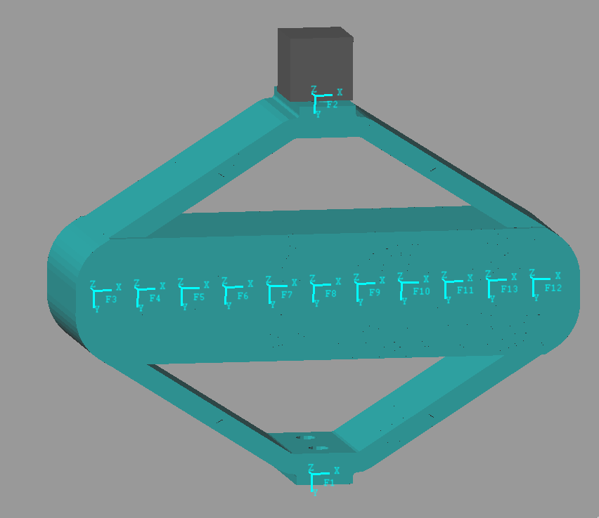
The flexible element is imported using the Reduced Order Flexible Solid simscape block.

To model the actuator, an Internal Force block is added between the nodes 3 and 12. A Relative Motion Sensor block is added between the nodes 1 and 2 to measure the displacement and the amplified piezo.

One mass is fixed at one end of the piezo-electric stack actuator, the other end is fixed to the world frame.

We first set the mass to be zero.

  m = 0.01;

The dynamics is identified from the applied force to the measured relative displacement.

  %% Name of the Simulink File
  mdl = 'piezo_amplified_3d';

  %% Input/Output definition
  clear io; io_i = 1;
  io(io_i) = linio([mdl, '/F'], 1, 'openinput');  io_i = io_i + 1;
  io(io_i) = linio([mdl, '/y'], 1, 'openoutput'); io_i = io_i + 1;

  Gh = -linearize(mdl, io);

Then, we add 10Kg of mass:

  m = 5;

And the dynamics is identified.

The two identified dynamics are compared in Figure fig:dynamics_act_disp_comp_mass.

  %% Name of the Simulink File
  mdl = 'piezo_amplified_3d';

  %% Input/Output definition
  clear io; io_i = 1;
  io(io_i) = linio([mdl, '/F'], 1, 'openinput');  io_i = io_i + 1;
  io(io_i) = linio([mdl, '/y'], 1, 'openoutput'); io_i = io_i + 1;

  Ghm = -linearize(mdl, io);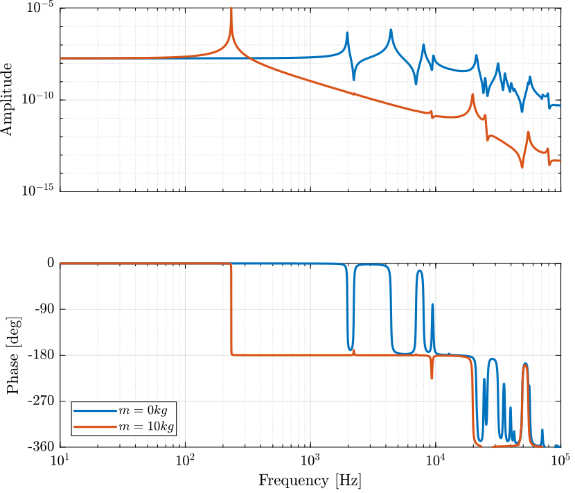

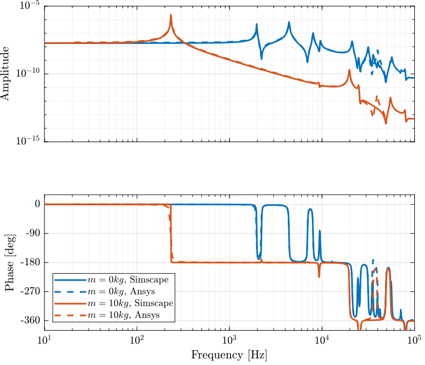
Dynamics from $F$ to $d$ without a payload and with a 10kg payload

Comparison with Ansys

Let's import the results from an Harmonic response analysis in Ansys.

  Gresp0 = readtable('FEA_HarmResponse_00kg.txt');
  Gresp10 = readtable('FEA_HarmResponse_10kg.txt');

The obtained dynamics from the Simscape model and from the Ansys analysis are compare in Figure fig:dynamics_force_disp_comp_anasys.

Comparison of the obtained dynamics using Simscape with the harmonic response analysis using Ansys

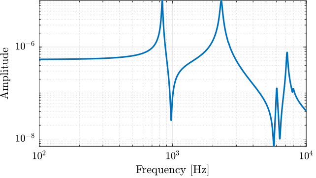
Force Sensor

The dynamics is identified from internal forces applied between nodes 3 and 11 to the relative displacement of nodes 11 and 13.

The obtained dynamics is shown in Figure fig:dynamics_force_force_sensor_comp_mass.

  m = 0;

  %% Name of the Simulink File
  mdl = 'piezo_amplified_3d';

  %% Input/Output definition
  clear io; io_i = 1;
  io(io_i) = linio([mdl, '/Fa'], 1, 'openinput');  io_i = io_i + 1;
  io(io_i) = linio([mdl, '/Fs'], 1, 'openoutput'); io_i = io_i + 1;

  Gf = linearize(mdl, io);

  m = 10;

  %% Name of the Simulink File
  mdl = 'piezo_amplified_3d';

  %% Input/Output definition
  clear io; io_i = 1;
  io(io_i) = linio([mdl, '/Fa'], 1, 'openinput');  io_i = io_i + 1;
  io(io_i) = linio([mdl, '/Fs'], 1, 'openoutput'); io_i = io_i + 1;

  Gfm = linearize(mdl, io);

Dynamics from $F$ to $F_m$ for $m=0$ and $m = 10kg$

Distributed Actuator

  m = 0;

The dynamics is identified from the applied force to the measured relative displacement.

  %% Name of the Simulink File
  mdl = 'piezo_amplified_3d_distri';

  %% Input/Output definition
  clear io; io_i = 1;
  io(io_i) = linio([mdl, '/F'], 1, 'openinput');  io_i = io_i + 1;
  io(io_i) = linio([mdl, '/y'], 1, 'openoutput'); io_i = io_i + 1;

  Gd = linearize(mdl, io);

Then, we add 10Kg of mass:

  m = 10;

And the dynamics is identified.

  %% Name of the Simulink File
  mdl = 'piezo_amplified_3d_distri';

  %% Input/Output definition
  clear io; io_i = 1;
  io(io_i) = linio([mdl, '/F'], 1, 'openinput');  io_i = io_i + 1;
  io(io_i) = linio([mdl, '/y'], 1, 'openoutput'); io_i = io_i + 1;

  Gdm = linearize(mdl, io);

Distributed Actuator and Force Sensor

  m = 0;

  %% Name of the Simulink File
  mdl = 'piezo_amplified_3d_distri_act_sens';

  %% Input/Output definition
  clear io; io_i = 1;
  io(io_i) = linio([mdl, '/F'], 1, 'openinput');  io_i = io_i + 1;
  io(io_i) = linio([mdl, '/Fm'], 1, 'openoutput'); io_i = io_i + 1;

  Gfd = linearize(mdl, io);

  m = 10;

  %% Name of the Simulink File
  mdl = 'piezo_amplified_3d_distri_act_sens';

  %% Input/Output definition
  clear io; io_i = 1;
  io(io_i) = linio([mdl, '/F'], 1, 'openinput');  io_i = io_i + 1;
  io(io_i) = linio([mdl, '/Fm'], 1, 'openoutput'); io_i = io_i + 1;

  Gfdm = linearize(mdl, io);

Dynamics from input voltage to displacement

  m = 5;

And the dynamics is identified.

The two identified dynamics are compared in Figure fig:dynamics_act_disp_comp_mass.

  %% Name of the Simulink File
  mdl = 'piezo_amplified_3d';

  %% Input/Output definition
  clear io; io_i = 1;
  io(io_i) = linio([mdl, '/V'], 1, 'openinput');  io_i = io_i + 1;
  io(io_i) = linio([mdl, '/y'], 1, 'openoutput'); io_i = io_i + 1;

  G = -linearize(mdl, io);

  save('../test-bench-apa/mat/fem_model_5kg.mat', 'G')

Dynamics from input voltage to output voltage

  m = 5;

  %% Name of the Simulink File
  mdl = 'piezo_amplified_3d';

  %% Input/Output definition
  clear io; io_i = 1;
  io(io_i) = linio([mdl, '/Va'], 1, 'openinput');  io_i = io_i + 1;
  io(io_i) = linio([mdl, '/Vs'], 1, 'openoutput'); io_i = io_i + 1;

  G = -linearize(mdl, io);

APA300ML

Introduction   ignore

Ansys FEM of the APA300ML

Import Mass Matrix, Stiffness Matrix, and Interface Nodes Coordinates

We first extract the stiffness and mass matrices.

  K = extractMatrix('mat_K-48modes-7MDoF.matrix');
  M = extractMatrix('mat_M-48modes-7MDoF.matrix');

  K = extractMatrix('mat_K-80modes-7MDoF.matrix');
  M = extractMatrix('mat_M-80modes-7MDoF.matrix');

Then, we extract the coordinates of the interface nodes.

  [int_xyz, int_i, n_xyz, n_i, nodes] = extractNodes('Nodes_MDoF_NLIST_MLIST.txt');

  save('./mat/APA300ML.mat', 'int_xyz', 'int_i', 'n_xyz', 'n_i', 'nodes', 'M', 'K');

Output parameters

  load('./mat/APA300ML.mat', 'int_xyz', 'int_i', 'n_xyz', 'n_i', 'nodes', 'M', 'K');

Total number of Nodes	7
Number of interface Nodes	7
Number of Modes	6
Size of M and K matrices	48

Node i	Node Number	x [m]	y [m]	z [m]
1.0	53917.0	0.0	-0.015	0.0
2.0	53918.0	0.0	0.015	0.0
3.0	53919.0	-0.0325	0.0	0.0
4.0	53920.0	-0.0125	0.0	0.0
5.0	53921.0	-0.0075	0.0	0.0
6.0	53922.0	0.0125	0.0	0.0
7.0	53923.0	0.0325	0.0	0.0

Coordinates of the interface nodes

200000000.0	30000.0	50000.0	200.0	-100.0	-300000.0	10000000.0	-6000.0	20000.0	-60.0
30000.0	7000000.0	10000.0	30.0	-30.0	-70.0	7000.0	-500000.0	3000.0	-10.0
50000.0	10000.0	30000000.0	200000.0	-200.0	-100.0	20000.0	-2000.0	2000000.0	-9000.0
200.0	30.0	200000.0	1000.0	-0.8	-0.4	50.0	-6	9000.0	-30.0
-100.0	-30.0	-200.0	-0.8	10000.0	0.2	-40.0	10.0	20.0	-0.05
-300000.0	-70.0	-100.0	-0.4	0.2	900.0	-30000.0	10.0	-40.0	0.1
10000000.0	7000.0	20000.0	50.0	-40.0	-30000.0	200000000.0	-50000.0	30000.0	-50.0
-6000.0	-500000.0	-2000.0	-6	10.0	10.0	-50000.0	7000000.0	-4000.0	8
20000.0	3000.0	2000000.0	9000.0	20.0	-40.0	30000.0	-4000.0	30000000.0	-200000.0
-60.0	-10.0	-9000.0	-30.0	-0.05	0.1	-50.0	8	-200000.0	1000.0

First 10x10 elements of the Stiffness matrix

0.01	7e-06	-5e-06	-6e-08	3e-09	-5e-05	-0.0005	-2e-07	-3e-06	1e-08
7e-06	0.009	4e-07	6e-09	-4e-09	-3e-08	-2e-07	6e-05	5e-07	-1e-09
-5e-06	4e-07	0.01	2e-05	2e-08	3e-08	-2e-06	-1e-07	-0.0002	9e-07
-6e-08	6e-09	2e-05	3e-07	1e-10	3e-10	-7e-09	2e-10	-9e-07	3e-09
3e-09	-4e-09	2e-08	1e-10	1e-07	-3e-12	6e-09	-2e-10	-3e-09	9e-12
-5e-05	-3e-08	3e-08	3e-10	-3e-12	6e-07	1e-06	-3e-09	2e-08	-7e-11
-0.0005	-2e-07	-2e-06	-7e-09	6e-09	1e-06	0.01	-8e-06	-2e-06	9e-09
-2e-07	6e-05	-1e-07	2e-10	-2e-10	-3e-09	-8e-06	0.009	1e-07	2e-09
-3e-06	5e-07	-0.0002	-9e-07	-3e-09	2e-08	-2e-06	1e-07	0.01	-2e-05
1e-08	-1e-09	9e-07	3e-09	9e-12	-7e-11	9e-09	2e-09	-2e-05	3e-07

First 10x10 elements of the Mass matrix

Using K, M and int_xyz, we can use the Reduced Order Flexible Solid simscape block.

Piezoelectric parameters

Parameters for the APA300ML:

  d33 = 3e-10; % Strain constant [m/V]
  n = 80; % Number of layers per stack
  eT = 1.6e-8; % Permittivity under constant stress [F/m]
  sD = 2e-11; % Elastic compliance under constant electric displacement [m2/N]
  ka = 235e6; % Stack stiffness [N/m]
  C = 5e-6; % Stack capactiance [F]

  na = 2; % Number of stacks used as actuator
  ns = 1; % Number of stacks used as force sensor

The ratio of the developed force to applied voltage is $d_{33} n k_a$ in [N/V]. We denote this constant by $g_a$ and: \[ F_a = g_a V_a, \quad g_a = d_{33} n k_a \]

  d33*(na*n)*(ka/(na + ns)) % [N/V]

0.42941

From cite:fleming14_desig_model_contr_nanop_system (page 123), the relation between relative displacement and generated voltage is: \[ V_s = \frac{d_{33}}{\epsilon^T s^D n} \Delta h \] where:

• $V_s$: measured voltage [V]
• $d_{33}$: strain constant [m/V]
• $\epsilon^T$: permittivity under constant stress [F/m]
• $s^D$: elastic compliance under constant electric displacement [m^2/N]
• $n$: number of layers
• $\Delta h$: relative displacement [m]

  1e-6*d33/(eT*sD*ns*n) % [V/um]

5.8594

Identification of the APA Characteristics

Stiffness

The transfer function from vertical external force to the relative vertical displacement is identified.

The inverse of its DC gain is the axial stiffness of the APA:

  1e-6/dcgain(G) % [N/um]

1.8634

The specified stiffness in the datasheet is $k = 1.8\, [N/\mu m]$.

Resonance Frequency

The resonance frequency is specified to be between 650Hz and 840Hz. This is also the case for the FEM model (Figure fig:apa300ml_resonance).

First resonance is around 800Hz

Amplification factor

The amplification factor is the ratio of the axial displacement to the stack displacement.

The ratio of the two displacement is computed from the FEM model.

  -dcgain(G(1,1))./dcgain(G(2,1))

4.936

If we take the ratio of the piezo height and length (approximation of the amplification factor):

  75/15

5

Stroke

Estimation of the actuator stroke: \[ \Delta H = A n \Delta L \] with:

• $\Delta H$ Axial Stroke of the APA
• $A$ Amplification factor (5 for the APA300ML)
• $n$ Number of stack used
• $\Delta L$ Stroke of the stack (0.1% of its length)

  1e6 * 5 * 3 * 20e-3 * 0.1e-2

300

This is exactly the specified stroke in the data-sheet.

Identification of the Dynamics

The flexible element is imported using the Reduced Order Flexible Solid simscape block.

To model the actuator, an Internal Force block is added between the nodes 3 and 12. A Relative Motion Sensor block is added between the nodes 1 and 2 to measure the displacement and the amplified piezo.

One mass is fixed at one end of the piezo-electric stack actuator, the other end is fixed to the world frame.

We first set the mass to be zero.

The dynamics is identified from the applied force to the measured relative displacement.

The same dynamics is identified for a payload mass of 10Kg.

  m = 10;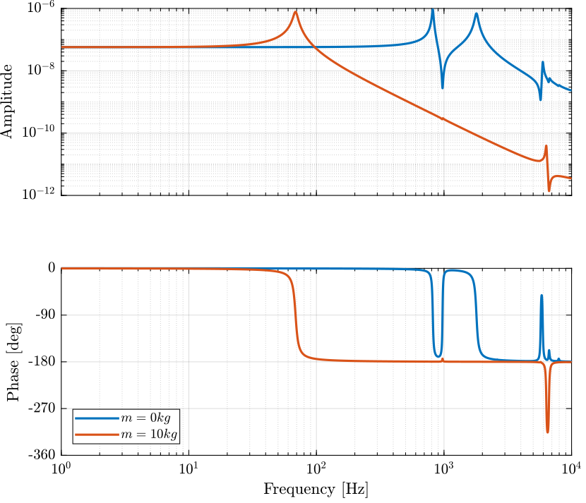

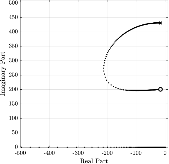
Transfer function from forces applied by the stack to the axial displacement of the APA

IFF

Let's use 2 stacks as actuators and 1 stack as force sensor.

The transfer function from actuator to sensors is identified and shown in Figure fig:apa300ml_iff_plant.

Transfer function from actuator to force sensor

For root locus corresponding to IFF is shown in Figure fig:apa300ml_iff_root_locus.

Root Locus for IFF

DVF

Now the dynamics from the stack actuator to the relative motion sensor is identified and shown in Figure fig:apa300ml_dvf_plant.

Transfer function from stack actuator to relative motion sensor

The root locus for DVF is shown in Figure fig:apa300ml_dvf_root_locus.

Root Locus for Direct Velocity Feedback

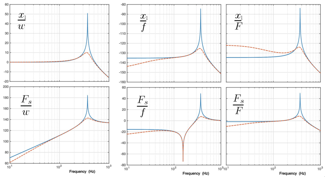
Identification for a simpler model

The goal in this section is to identify the parameters of a simple APA model from the FEM. This can be useful is a lower order model is to be used for simulations.

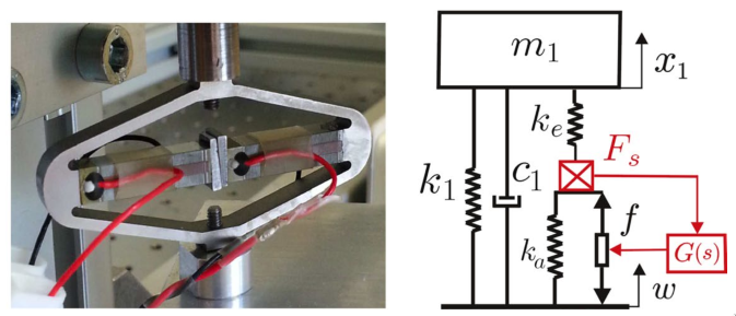
The presented model is based on cite:souleille18_concep_activ_mount_space_applic.

The model represents the Amplified Piezo Actuator (APA) from Cedrat-Technologies (Figure fig:souleille18_model_piezo). The parameters are shown in the table below.

Picture of an APA100M from Cedrat Technologies. Simplified model of a one DoF payload mounted on such isolator

	Meaning
$k_e$	Stiffness used to adjust the pole of the isolator
$k_1$	Stiffness of the metallic suspension when the stack is removed
$k_a$	Stiffness of the actuator
$c_1$	Added viscous damping

Parameters used for the model of the APA 100M

The goal is to determine $k_e$, $k_a$ and $k_1$ so that the simplified model fits the FEM model.

\[ \alpha = \frac{x_1}{f}(\omega=0) = \frac{\frac{k_e}{k_e + k_a}}{k_1 + \frac{k_e k_a}{k_e + k_a}} \] \[ \beta = \frac{x_1}{F}(\omega=0) = \frac{1}{k_1 + \frac{k_e k_a}{k_e + k_a}} \]

If we can fix $k_a$, we can determine $k_e$ and $k_1$ with: \[ k_e = \frac{k_a}{\frac{\beta}{\alpha} - 1} \] \[ k_1 = \frac{1}{\beta} - \frac{k_e k_a}{k_e + k_a} \]

From the identified dynamics, compute $\alpha$ and $\beta$

  alpha = abs(dcgain(G('y', 'Fa')));
  beta  = abs(dcgain(G('y', 'Fd')));

$k_a$ is estimated using the following formula:

  ka = 0.8/abs(dcgain(G('y', 'Fa')));

The factor can be adjusted to better match the curves.

Then $k_e$ and $k_1$ are computed.

  ke = ka/(beta/alpha - 1);
  k1 = 1/beta - ke*ka/(ke + ka);

	Value [N/um]
ka	42.9
ke	1.5
k1	0.4

The damping in the system is adjusted to match the FEM model if necessary.

  c1 = 1e2;

Analytical model of the simpler system:

  Ga = 1/(m*s^2 + k1 + c1*s + ke*ka/(ke + ka)) * ...
       [ 1 ,              k1 + c1*s + ke*ka/(ke + ka)  , ke/(ke + ka) ;
        -ke*ka/(ke + ka), ke*ka/(ke + ka)*m*s^2 ,       -ke/(ke + ka)*(m*s^2 + c1*s + k1)];

  Ga.InputName = {'Fd', 'w', 'Fa'};
  Ga.OutputName = {'y', 'Fs'};

Adjust the DC gain for the force sensor:

  lambda = dcgain(Ga('Fs', 'Fd'))/dcgain(G('Fs', 'Fd'));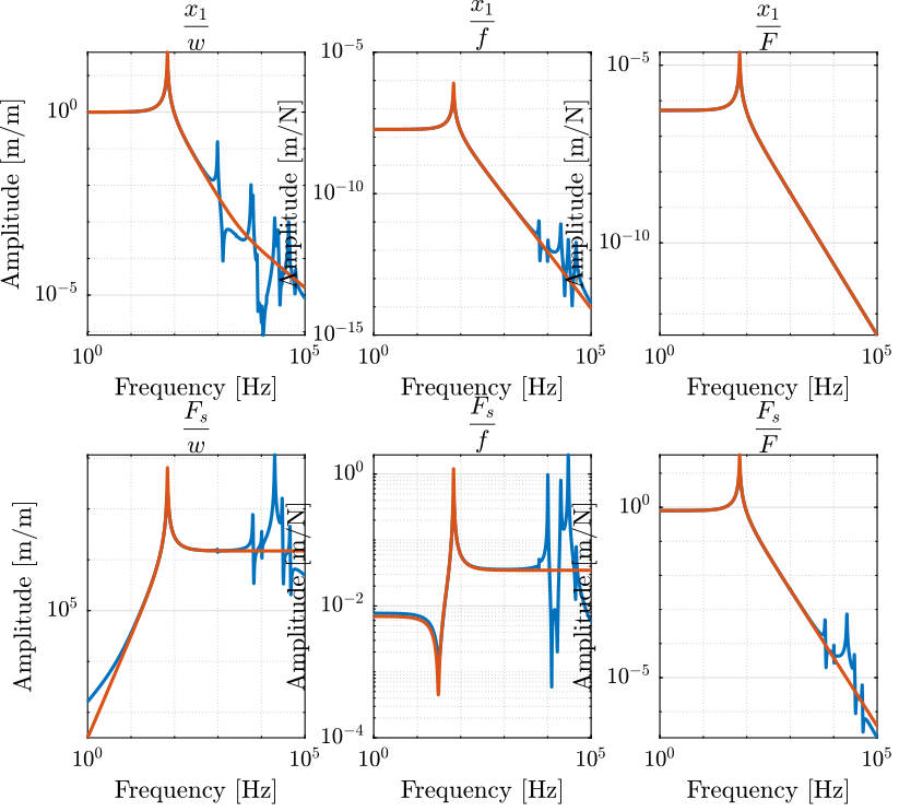

Comparison of the Dynamics between the FEM model and the simplified one

Flexible Joint

Introduction   ignore

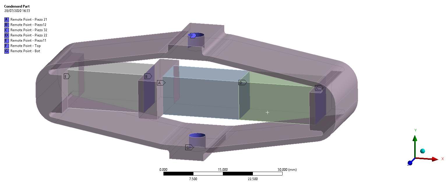
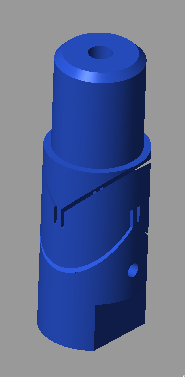
The flexor in Figure fig:flexor_id16_screenshot is studied with a FEM.

Flexor studied

Import Mass Matrix, Stiffness Matrix, and Interface Nodes Coordinates

We first extract the stiffness and mass matrices.

  K = extractMatrix('mat_K_6modes_2MDoF.matrix');
  M = extractMatrix('mat_M_6modes_2MDoF.matrix');

Then, we extract the coordinates of the interface nodes.

  [int_xyz, int_i, n_xyz, n_i, nodes] = extractNodes('out_nodes_3D.txt');

  save('./mat/flexor_ID16.mat', 'int_xyz', 'int_i', 'n_xyz', 'n_i', 'nodes', 'M', 'K');

Output parameters

  load('./mat/flexor_ID16.mat', 'int_xyz', 'int_i', 'n_xyz', 'n_i', 'nodes', 'M', 'K');

Total number of Nodes	2
Number of interface Nodes	2
Number of Modes	6
Size of M and K matrices	18

Node i	Node Number	x [m]	y [m]	z [m]
1.0	181278.0	0.0	0.0	0.0
2.0	181279.0	0.0	0.0	-0.0

Coordinates of the interface nodes

11200000.0	195.0	2220.0	-0.719	-265.0	1.59	-11200000.0	-213.0	-2220.0	0.147
195.0	11400000.0	1290.0	-148.0	-0.188	2.41	-212.0	-11400000.0	-1290.0	148.0
2220.0	1290.0	119000000.0	1.31	1.49	1.79	-2220.0	-1290.0	-119000000.0	-1.31
-0.719	-148.0	1.31	33.0	0.000488	-0.000977	0.141	148.0	-1.31	-33.0
-265.0	-0.188	1.49	0.000488	33.0	0.00293	266.0	0.154	-1.49	0.00026
1.59	2.41	1.79	-0.000977	0.00293	236.0	-1.32	-2.55	-1.79	0.000379
-11200000.0	-212.0	-2220.0	0.141	266.0	-1.32	11400000.0	24600.0	1640.0	120.0
-213.0	-11400000.0	-1290.0	148.0	0.154	-2.55	24600.0	11400000.0	1290.0	-72.0
-2220.0	-1290.0	-119000000.0	-1.31	-1.49	-1.79	1640.0	1290.0	119000000.0	1.32
0.147	148.0	-1.31	-33.0	0.00026	0.000379	120.0	-72.0	1.32	34.7

First 10x10 elements of the Stiffness matrix

0.02	1e-09	-4e-08	-1e-10	0.0002	-3e-11	0.004	5e-08	7e-08	1e-10
1e-09	0.02	-3e-07	-0.0002	-1e-10	-2e-09	2e-08	0.004	3e-07	1e-05
-4e-08	-3e-07	0.02	7e-10	-2e-09	1e-09	3e-07	7e-08	0.003	1e-09
-1e-10	-0.0002	7e-10	4e-06	-1e-12	-6e-13	2e-10	-7e-06	-8e-10	-1e-09
0.0002	-1e-10	-2e-09	-1e-12	3e-06	2e-13	9e-06	4e-11	2e-09	-3e-13
-3e-11	-2e-09	1e-09	-6e-13	2e-13	4e-07	8e-11	9e-10	-1e-09	2e-12
0.004	2e-08	3e-07	2e-10	9e-06	8e-11	0.02	-7e-08	-3e-07	-2e-10
5e-08	0.004	7e-08	-7e-06	4e-11	9e-10	-7e-08	0.01	-4e-08	0.0002
7e-08	3e-07	0.003	-8e-10	2e-09	-1e-09	-3e-07	-4e-08	0.02	-1e-09
1e-10	1e-05	1e-09	-1e-09	-3e-13	2e-12	-2e-10	0.0002	-1e-09	2e-06

First 10x10 elements of the Mass matrix

Using K, M and int_xyz, we can use the Reduced Order Flexible Solid simscape block.

Flexible Joint Characteristics

The most important parameters of the flexible joint can be directly estimated from the stiffness matrix.

Caracteristic	Value	Estimation by Francois
Axial Stiffness [N/um]	119	60
Bending Stiffness [Nm/rad]	33	15
Bending Stiffness [Nm/rad]	33	15
Torsion Stiffness [Nm/rad]	236	20

Identification of the parameters using Simscape

The flexor is now imported into Simscape and its parameters are estimated using an identification.

The dynamics is identified from the applied force/torque to the measured displacement/rotation of the flexor.

And we find the same parameters as the one estimated from the Stiffness matrix.

Caracteristic	Value	Identification
Axial Stiffness Dz [N/um]	119	119
Bending Stiffness Rx [Nm/rad]	33	33
Bending Stiffness Ry [Nm/rad]	33	33
Torsion Stiffness Rz [Nm/rad]	236	236

Simpler Model

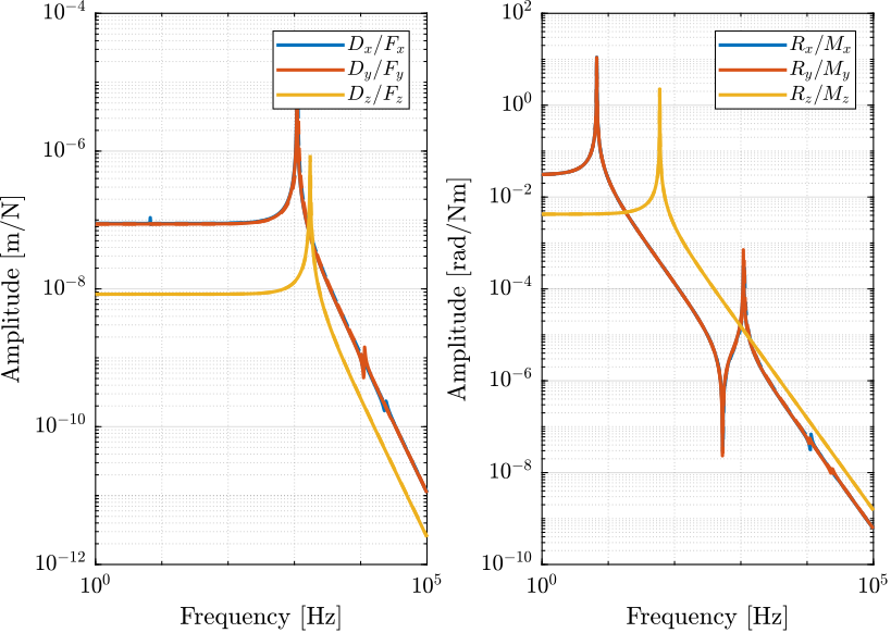
Let's now model the flexible joint with a "perfect" Bushing joint as shown in Figure fig:flexible_joint_simscape.

Bushing Joint used to model the flexible joint

The parameters of the Bushing joint (stiffnesses) are estimated from the Stiffness matrix that was computed from the FEM.

  Kx = K(1,1); % [N/m]
  Ky = K(2,2); % [N/m]
  Kz = K(3,3); % [N/m]
  Krx = K(4,4); % [Nm/rad]
  Kry = K(5,5); % [Nm/rad]
  Krz =  K(6,6); % [Nm/rad]

The dynamics from the applied force/torque to the measured displacement/rotation of the flexor is identified again for this simpler model.

The two obtained dynamics are compared in Figure

Comparison of the Joint compliance between the FEM model and the simpler model

Integral Force Feedback with Amplified Piezo

Introduction   ignore

In this section, we try to replicate the results obtained in cite:souleille18_concep_activ_mount_space_applic.

Import Mass Matrix, Stiffness Matrix, and Interface Nodes Coordinates

We first extract the stiffness and mass matrices.

  K = extractMatrix('piezo_amplified_IFF_K.txt');
  M = extractMatrix('piezo_amplified_IFF_M.txt');

Then, we extract the coordinates of the interface nodes.

  [int_xyz, int_i, n_xyz, n_i, nodes] = extractNodes('piezo_amplified_IFF.txt');

IFF Plant

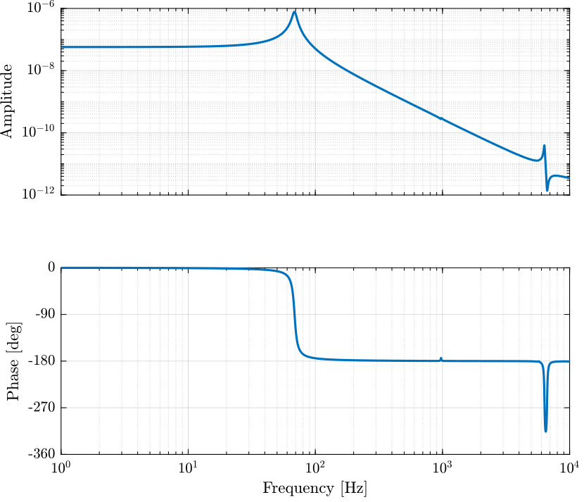
The transfer function from the force actuator to the force sensor is identified and shown in Figure fig:piezo_amplified_iff_plant.

  Kiff = tf(0);

  m = 0;

  %% Name of the Simulink File
  mdl = 'piezo_amplified_IFF';

  %% Input/Output definition
  clear io; io_i = 1;
  io(io_i) = linio([mdl, '/Kiff'], 1, 'openinput');  io_i = io_i + 1;
  io(io_i) = linio([mdl, '/G'],    1, 'openoutput'); io_i = io_i + 1;

  Gf = linearize(mdl, io);

  m = 10;

  Gfm = linearize(mdl, io);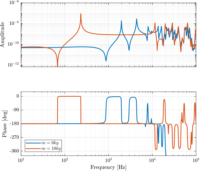

IFF Plant

IFF controller

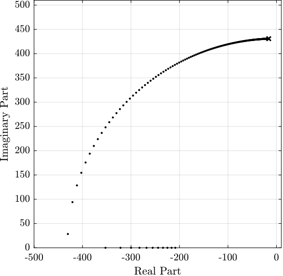
The controller is defined and the loop gain is shown in Figure fig:piezo_amplified_iff_loop_gain.

  Kiff = -1e12/s;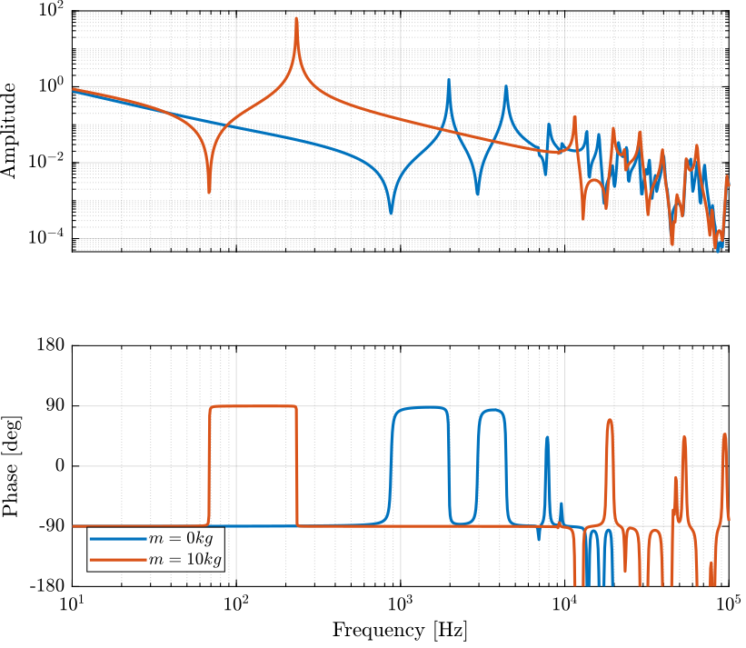

IFF Loop Gain

Closed Loop System

  m = 10;

  Kiff = -1e12/s;

  %% Name of the Simulink File
  mdl = 'piezo_amplified_IFF';

  %% Input/Output definition
  clear io; io_i = 1;
  io(io_i) = linio([mdl, '/Dw'], 1, 'openinput');  io_i = io_i + 1;
  io(io_i) = linio([mdl, '/F'],  1, 'openinput');  io_i = io_i + 1;
  io(io_i) = linio([mdl, '/Fd'], 1, 'openinput');  io_i = io_i + 1;
  io(io_i) = linio([mdl, '/d'],  1, 'openoutput'); io_i = io_i + 1;
  io(io_i) = linio([mdl, '/G'],  1, 'output'); io_i = io_i + 1;

  Giff = linearize(mdl, io);
  Giff.InputName  = {'w', 'f', 'F'};
  Giff.OutputName  = {'x1', 'Fs'};

  Kiff = tf(0);

  G = linearize(mdl, io);
  G.InputName  = {'w', 'f', 'F'};
  G.OutputName  = {'x1', 'Fs'};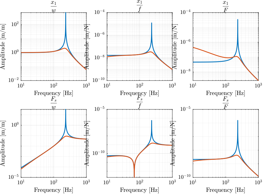

OL and CL transfer functions

Results obtained in cite:souleille18_concep_activ_mount_space_applic

Bibliography   ignore

bibliographystyle:unsrt bibliography:ref.bib