phd-nass-fem/nass-fem.org

Optimization using Finite Element Models

• Introduction
• Reduced order flexible bodies
  • Introduction
  • Procedure
  • Example with an Amplified Piezoelectric Actuator
    • Introduction
    • Finite Element Model
    • Super Element in the Multi-Body Model
    • Sensor and Actuator "constants"
  • Experimental Validation
    • Introduction
    • Test Bench
    • Comparison of the dynamics
    • Integral Force Feedback with APA
  • Conclusion
• Actuator
  • Introduction
  • Choice of the Actuator based on Specifications
  • APA300ML - Reduced Order Flexible Body
  • Identification of the APA Characteristics
    • Introduction
    • Stiffness
    • Resonance Frequency
    • Amplification Factor and Actuator Stroke
  • Simpler 2DoF Model of the APA300ML
    • Introduction
    • 2DoF Model
    • Parameter Tuning
  • Electrical characteristics of the APA
  • Validation with the Nano-Hexapod
• Flexible Joint
  • Introduction
  • Flexible joints for Stewart platforms
  • Bending and Torsional Stiffness
  • Axial Stiffness
  • Obtained design / Specifications
  • Validation with the Nano-Hexapod
• Conclusion
• Bibliography
• Footnotes

Introduction   ignore

• In the detail design phase, one goal is to optimize the design of the nano-hexapod
• Parts are usually optimized using Finite Element Models that are used to estimate the static and dynamical properties of parts
• However, it is important to see how to dynamics of each part combines with the nano-hexapod and with the micro-station. One option would be to use a FEM of the complete NASS, but that would be very complex and it would be difficult to perform simulations of experiments with real time control implemented.

• The idea is therefore to combine FEM with the multi body model of the NASS. To do so, Reduced Order Flexible Bodies are used (Section ref:sec:detail_fem_super_element)

  • The theory is described
  • The method is validated using experimental measurements

• Two main elements of the nano-hexapod are then optimized:

  • The actuator (Section ref:sec:detail_fem_actuator)
  • The flexible joints (Section ref:sec:detail_fem_joint)

Reduced order flexible bodies

<<sec:detail_fem_super_element>>

Introduction   ignore

Components exhibiting complex dynamical behavior are frequently found to be unsuitable for direct implementation within multi-body models. These components are traditionally analyzed using Finite Element Analysis (FEA) software. However, a methodological bridge between these two analytical approaches has been established, whereby components whose dynamical properties have been determined through FEA can be successfully integrated into multi-body models cite:&hatch00_vibrat_matlab_ansys. This combined multibody-FEA modeling approach presents significant advantages, as it enables the selective application of FEA modeling to specific elements while maintaining the computational efficiency of multi-body analysis for the broader system cite:&rankers98_machin.

The investigation of this hybrid modeling approach is structured in three sections. First, the fundamental principles and methodological approaches of this modeling framework are introduced (Section ref:ssec:detail_fem_super_element_theory). It is then illustrated through its practical application to the modelling of an Amplified Piezoelectric Actuator (APA) (Section ref:ssec:detail_fem_super_element_example). Finally, the validity of this modeling approach is demonstrated through experimental validation, wherein the obtained dynamics from the hybrid modelling approach is compared with measurements (Section ref:ssec:detail_fem_super_element_validation).

The work presented in this section has also been published in cite:&brumund21_multib_simul_reduc_order_flexib_bodies_fea.

Procedure

<<ssec:detail_fem_super_element_theory>>

In this modeling approach, some components within the multi-body framework are represented as reduced-order flexible bodies, wherein their modal behavior is characterized through reduced mass and stiffness matrices derived from finite element analysis (FEA) models. These matrices are generated via modal reduction techniques, specifically through the application of component mode synthesis (CMS), thus establishing this design approach as a combined multibody-FEA methodology.

Standard FEA implementations typically involve thousands or even hundreds of thousands of DoF, rendering direct integration into multi-body simulations computationally prohibitive. The objective of modal reduction is therefore to substantially decrease the number of DoF while preserving the essential dynamic characteristics of the component.

The procedure for implementing this reduction involves several distinct stages. Initially, the component is modeled in a finite element software with appropriate material properties and boundary conditions. Subsequently, interface frames are defined at locations where the multi-body model will establish connections with the component. These frames serve multiple functions, including connecting to other parts, applying forces and torques, and measuring relative motion between defined frames.

Following the establishment of these interface parameters, modal reduction is performed using the Craig-Bampton method cite:&craig68_coupl_subst_dynam_analy (also known as the "fixed-interface method"), a technique that transforms the extensive FEA degrees of freedom into a significantly reduced set of retained degrees of freedom. This transformation typically reduces the model complexity from hundreds of thousands to fewer than 100 DoF. The number of degrees of freedom in the reduced model is determined by eqref:eq:detail_fem_model_order where $n$ represents the number of defined frames and $p$ denotes the number of additional modes to be modeled. The outcome of this procedure is an $m \times m$ set of reduced mass and stiffness matrices, which can subsequently be incorporated into the multi-body model to represent the component's dynamic behavior.

\begin{equation}\label{eq:detail_fem_model_order} m = 6 × n + p

\end{equation}

Example with an Amplified Piezoelectric Actuator

<<ssec:detail_fem_super_element_example>>

Introduction   ignore

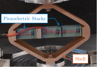
The presented modeling framework was first applied to an Amplified Piezoelectric Actuator (APA) for several reasons. Primarily, this actuator represents an excellent candidate for implementation within the nano-hexapod, as will be elaborated in Section ref:sec:detail_fem_actuator. Additionally, an Amplified Piezoelectric Actuator (the APA95ML shown in Figure ref:fig:detail_fem_apa95ml_picture) was available in the laboratory for experimental testing.

The APA consists of multiple piezoelectric stacks arranged horizontally (depicted in blue in Figure ref:fig:detail_fem_apa95ml_picture) and an amplifying shell structure (shown in red) that serves two purposes: the application of pre-stress to the piezoelectric elements and the amplification of their displacement into the vertical direction cite:&claeyssen07_amplif_piezoel_actuat. The selection of the APA for validation purposes was further justified by its capacity to simultaneously demonstrate multiple aspects of the modeling framework. The specific design of the APA allows for the simultaneous modeling of a mechanical structure analogous to a flexible joint, piezoelectric actuation, and piezoelectric sensing, thereby encompassing the principal elements requiring validation.

\hfill

Parameter	Value
Nominal Stroke	$100\,\mu m$
Blocked force	$1600\,N$
Stiffness	$16\,N/\mu m$

Finite Element Model

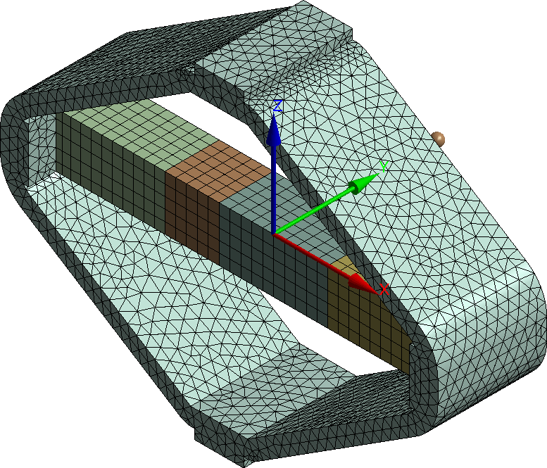
The development of the finite element model for the APA95ML necessitated the specification of appropriate material properties, as summarized in Table ref:tab:detail_fem_material_properties. The finite element mesh, shown in Figure ref:fig:detail_fem_apa95ml_mesh, was then generated.

	$E$	$\nu$	$\rho$
Stainless Steel	$190\,GPa$	$0.31$	$7800\,\text{kg}/m^3$
Piezoelectric Ceramics (PZT)	$49.5\,GPa$	$0.31$	$7800\,\text{kg}/m^3$

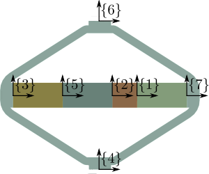
The definition of interface frames, or "remote points" as depicted in Figure ref:fig:detail_fem_apa95ml_frames, constitute a critical aspect of the model preparation. Seven frames were established: two frames for each piezoelectric stack to facilitate strain measurement and force application, and additional frames at the top and bottom of the structure to enable connection with external elements in the multi-body simulation.

Six additional modes were considered, resulting in total model order of $48$. The modal reduction procedure was then executed, yielding the reduced mass and stiffness matrices that form the foundation of the component's representation in the multi-body simulation environment.

Super Element in the Multi-Body Model

Model:

• Connect frame $\{4\}$ to world frame and frame $\{6\}$ to a 5.5kg mass, vertically guided

• 2 actuator stacks, 1 sensor stack:

  • force source between frames $\{3\}$ and $\{2\}$
  • measured strain for force sensor by measuring the displacement between $\{1\}$ and $\{7\}$
• Input: internal force applied
• Output: strain in the sensor stack
• Issue: how to convert voltage to force and strain to voltage?

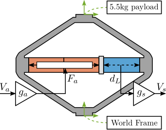
Need to link the electrical domain (voltages, charges) with the mechanical domain (forces, strain). To do so, "actuator constant" $g_a$ and "sensor constant" $g_s$ are used as shown in Figure ref:fig:detail_fem_apa_model_schematic.

A voltage $V_a$ applied to the actuator stacks will induce an actuator force $F_a$:

\begin{equation} \boxed{F_a = g_a \cdot V_a} \end{equation}

A change of length $dl$ of the sensor stack will induce a voltage $V_s$:

\begin{equation} \boxed{V_s = g_s \cdot dl} \end{equation}

In order to correctly model the piezoelectric actuator with Simscape, the values for $g_a$ and $g_s$ needs to be determined.

• $g_a$: the ratio of the generated force $F_a$ to the supply voltage $V_a$ across the piezoelectric stack
• $g_s$: the ratio of the generated voltage $V_s$ across the piezoelectric stack when subject to a strain $\Delta h$

Sensor and Actuator "constants"

The gains $g_a$ and $g_s$ were estimated from the physical properties of the piezoelectric stack material (summarized in Table ref:tab:detail_fem_stack_parameters).

Parameter	Unit	Value
Nominal Stroke	$\mu m$	20
Blocked force	$N$	4700
Stiffness	$N/\mu m$	235
Voltage Range	$V$	-20 to 150
Capacitance	$\mu F$	4.4
Length	$mm$	20
Stack Area	$mm^2$	10x10

From cite:&fleming14_desig_model_contr_nanop_system p. 123, the relation between relative displacement $d_L$ of the sensor stack and generated voltage $V_s$ is given by eqref:eq:test_apa_piezo_strain_to_voltage and from cite:&fleming10_integ_strain_force_feedb_high the relation between the force $F_a$ and the applied voltage $V_a$ is given by eqref:eq:test_apa_piezo_voltage_to_force.

\begin{subequations} \begin{align} V_s &= \underbrace{\frac{d_{33}}{\epsilon^T s^D n}}_{g_s} d_L \label{eq:test_apa_piezo_strain_to_voltage} \\ F_a &= \underbrace{d_{33} n k_a}_{g_a} \cdot V_a, \quad k_a = \frac{c^{E} A}{L} \label{eq:test_apa_piezo_voltage_to_force} \end{align} \end{subequations}

Unfortunately, it is difficult to know exactly which material is used in the amplified piezoelectric actuator¹. However, based on the available properties of the stacks in the data-sheet (summarized in Table ref:tab:detail_fem_stack_parameters), the soft Lead Zirconate Titanate "THP5H" from Thorlabs seemed to match quite well the observed properties. The properties of this "THP5H" material used to compute $g_a$ and $g_s$ are listed in Table ref:tab:test_apa_piezo_properties.

From these parameters, $g_s = 5.1\,V/\mu m$ and $g_a = 26\,N/V$ were obtained.

Parameter	Value	Description
$d_{33}$	$680 \cdot 10^{-12}\,m/V$	Piezoelectric constant
$\epsilon^{T}$	$4.0 \cdot 10^{-8}\,F/m$	Permittivity under constant stress
$s^{D}$	$21 \cdot 10^{-12}\,m^2/N$	Elastic compliance understand constant electric displacement
$c^{E}$	$48 \cdot 10^{9}\,N/m^2$	Young's modulus of elasticity
$L$	$20\,mm$ per stack	Length of the stack
$A$	$10^{-4}\,m^2$	Area of the piezoelectric stack
$n$	$160$ per stack	Number of layers in the piezoelectric stack

%% Estimate "Sensor Constant" - (THP5H)
d33 = 680e-12;        % Strain constant [m/V]
n   = 160;            % Number of layers per stack
eT  = 4500*8.854e-12; % Permittivity under constant stress [F/m]
sD  = 21e-12;         % Compliance under constant electric displacement [m2/N]

gs = d33/(eT*sD*n);   % Sensor Constant [V/m]

%% Estimate "Actuator Constant" - (THP5H)
d33 = 680e-12;   % Strain constant [m/V]
n   = 320;       % Number of layers

cE  = 1/sD;      % Youngs modulus [N/m^2]
A   = (10e-3)^2; % Area of the stacks [m^2]
L   = 40e-3;     % Length of the two stacks [m]
ka  = cE*A/L;    % Stiffness of the two stacks [N/m]

ga = d33*n*ka;   % Actuator Constant [N/V]

Experimental Validation

<<ssec:detail_fem_super_element_validation>>

Introduction   ignore

Test Bench

goal: validation of the procedure.

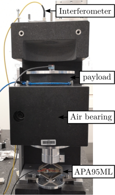
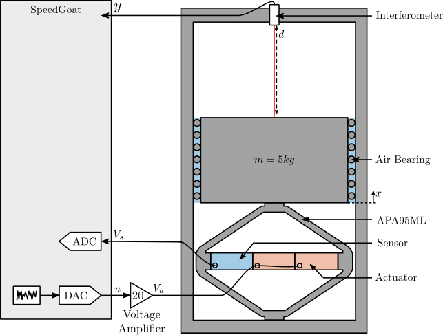
• Explain test bench: (Figure ref:fig:detail_fem_apa95ml_bench)

  • 5.7kg granite, vertical guided with an air bearing
  • fibered interferometer measured the vertical motion of the granite $y$
  • DAC generating control signal $u$, voltage amplifier gain of 20, $V_a$ is the voltage across the two piezoelectric stacks
  • ADC is used to measured the voltage across the piezoelectric sensor stack

Comparison of the dynamics

• Explain how to experimentally measure the transfer function:

  • test signal, here noise
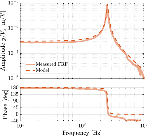
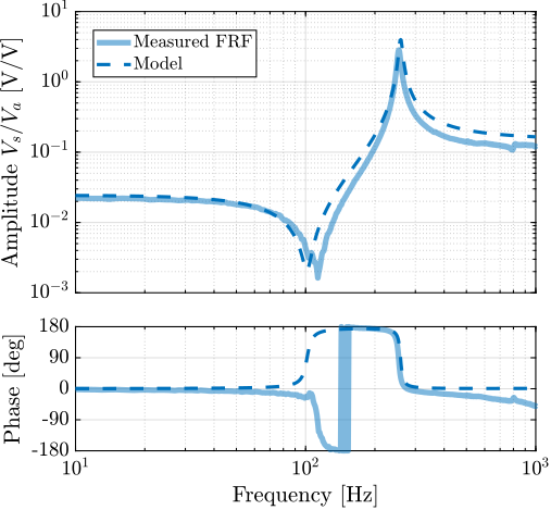
  • compute and show the transfer functions from $V_a$ to $y$ and to $V_s$
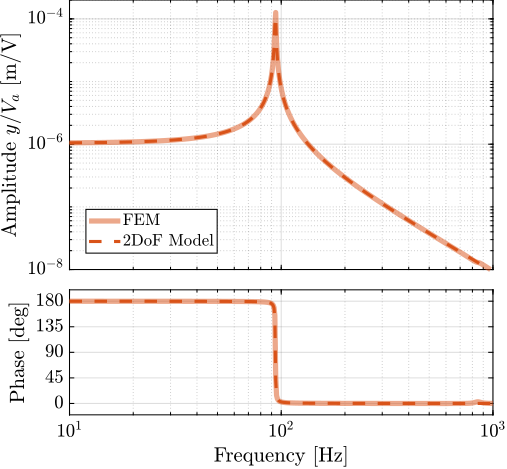
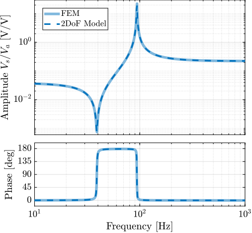
  • Compare the model and measurement: validation (Figure ref:fig:detail_fem_apa95ml_comp_plant)

  • talk about the phase:

    • for force sensor, just delay linked to the limited sampling rate of $0.1\,ms$
    • for interferometer: additional delay due to electronics being used
  • good match. The gains can be further tuned based on the experimental results.
  • talk about minimum phase zero: will be discussed during the experimental phase

%% Experimental plant identification
% with PD200 amplifier (gain of 20) - 2 stacks as an actuator, 1 as a sensor
load('apa95ml_5kg_2a_1s.mat')

Va = 20*u; % Voltage amplifier gain: 20

% Spectral Analysis parameters
Ts = t(end)/(length(t)-1);
Nfft = floor(1/Ts);
win = hanning(Nfft);
Noverlap = floor(Nfft/2);

% Identification of the transfer function from Va to di
[G_y,  f]  = tfestimate(detrend(Va, 0), detrend(y, 0), win, Noverlap, Nfft, 1/Ts);
[G_Vs, ~]  = tfestimate(detrend(Va, 0), detrend(v, 0), win, Noverlap, Nfft, 1/Ts);

%% Plant Identification from Multi-Body model
% Load Reduced Order Matrices
K = readmatrix('APA95ML_K.CSV'); % order: 48
M = readmatrix('APA95ML_M.CSV');
[int_xyz, int_i, n_xyz, n_i, nodes] = extractNodes('APA95ML_out_nodes_3D.txt');

m = 5.5; % Mass of the suspended granite [kg]

% Compute transfer functions
clear io; io_i = 1;
io(io_i) = linio([mdl, '/Va'], 1, 'openinput');  io_i = io_i + 1; % Voltage accros piezo stacks [V]
io(io_i) = linio([mdl, '/y'],  1, 'openoutput'); io_i = io_i + 1; % Vertical Displacement [m]
io(io_i) = linio([mdl, '/Vs'], 1, 'openoutput'); io_i = io_i + 1; % Sensor stack voltage [V]

Gm = linearize(mdl, io);
Gm.InputName  = {'Va'};
Gm.OutputName = {'y', 'Vs'};

Integral Force Feedback with APA

goal:

• validate the use of super element for control tasks

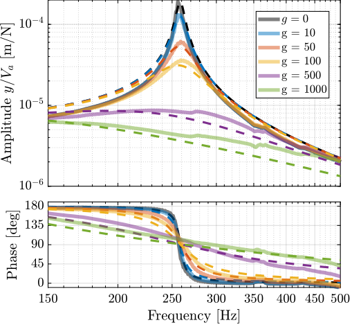
The controller used in the Integral Force Feedback Architecture is eqref:eq:detail_fem_iff_controller, wtih $g$ a gain that can be tuned.

\begin{equation}\label{eq:detail_fem_iff_controller} K_{\text{IFF}}(s) = \frac{g}{s + 2⋅ 2π} ⋅ \frac{s}{s + 0.5 ⋅ 2π}

\end{equation}

Above 2 Hz the controller is basically an integrator, whereas an high pass filter is added at 0.5Hz to further reduce the low frequency gain. In the frequency band of interest, this controller should mostly act as a pure integrator.

• Maybe make a block diagram of the control with added damped input

Conclusion

• Validation of the method
• Very useful to optimize different parts
• However, model order may become very large and not convenient to perform time domain simulations
• But extracting dynamics is not computational intensive, even for large model orders
• For instance APA: order 48, 6 APA for the nano hexapod 288 orders just for the APA

Actuator

<<sec:detail_fem_actuator>>

Introduction   ignore

Goals:

• Based on dynamical models and previous studies, extract specifications for the actuators to be included in the nano-hexapod. Then choose the most appropriate actuator based on specifications (Section ref:ssec:detail_fem_actuator_specifications)
• Model this actuator accurately using a "reduced order flexible body" to check the dynamics and validate the choice of actuator and validate this choice with simulations
• Development of a 2DoF model for lower order models (i.e. for simulations)

Choice of the Actuator based on Specifications

<<ssec:detail_fem_actuator_specifications>>

From previous analysis:

• Actuator stiffness has major impact on the system dynamics and performances due to several factors:

  • Spindle rotation: modification of plant dynamics and coupling increase due to Gyroscopic effects This require to have stiffness above ~
  • Limited micro-station compliance / complex dynamics: The actuator stiffness should be small enough such that the suspension modes of the nano-hexapod are below the problematic modes of the micro-stations.
  • There is therefore an intermediate stiffness that is foreseen to give the best compromise, and it is around $1\,N/\mu m$
• HAC-LAC strategy: Actuator must include a force sensor Because of the rotation, some stiffness should be present in parallel to the force sensor
• Limited space: As the maximum height of the nano-hexapod is 95mm, and each strut has a flexible joint at each end, it is estimated that the maximum height of the actuator should be less than 50mm
• Stroke: The stroke of the each actuator should be large enough such that the nano-hexapod mobility exceed the micro-station positioning errors. Some margins should be included for mounting errors, and further flexibility of the system (for instance to perform scans with the nano-hexapod, or to align the point of interest with the rotation axis)

Actuator specifications:

• Height (<50mm)
• Stroke (~100um)
• Stiffness (0.1-1 N/um)
• Blocked force?
• Force sensor

Options:

• Two main options: piezoelectric actuators and Lorentz actuator (also known as Voice coil actuators). Variable reluctance actuators were not considered, even though they have better efficiency than voice coil actuators, they are non linear and induce additional control complexity.

• Voice coil + relatively soft flexible guiding (1N/um):

  • required force ~100N for 100um correction This constant force/current would induce large thermal loads, that may negatively impact system's stability Advantages of voice coil (longer strokes than piezo + allow for very low stiffness in the direction of actuation, extremely linear for high performance feedforward) are not used here.

• Piezoelectric stack actuators:

  • PZT: stroke ~0.1% of its length.
  • 50mm length => 50um stroke which is barely enough
  • Extremely stiff, in the order of $100\,N/\mu m$, which is not wanted here.

• Amplified Piezoelectric Actuator:

  • shell is used to pre-stress the piezoelectric stacks and amplify the motion (roughly by the ratio of the width over the height)
  • This also reduce the stiffness in the direction of motion
  • This make this design quick compact in the direction of motion (i.e. in height)
  • When several stacks are used, one of them can be used as a force sensor, which is therefore very well collocated with the actuators
  • Therefore, this actuator is well suited for decentralized IFF, already applied for a Stewart platform with APA cite:&hanieh03_activ_stewar

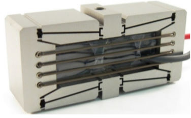
Based on previous analysis, it was decided to use amplified piezoelectric actuators for the nano-hexapod. Table ref:tab:detail_fem_piezo_act_models: compares few models that fulfill specifications. It was decided to go for the APA300ML (shown in Figure ref:fig:detail_fem_apa300ml_picture). One reason is that we already had experience with APA from Cedrat technologies, and the Finite Element Model was validated experimentally, so we are confident to model the APA300ML with FEA and include it in the NASS model for validation.

• Talk about piezoelectric actuator? bandwidth? noise?
• Resolution: really depends on the electrical noise (induced by DAC and voltage amplifier). They will be chosen appropriately

Specification	APA150M	APA300ML	APA400MML	FPA-0500E-P	FPA-0300E-S
Stroke $> 100\, [\mu m]$	187	304	368	432	240
Stiffness $\approx 1\, [N/\mu m]$	0.7	1.8	0.55	0.87	0.58
Resolution $< 2\, [nm]$	2	3	4
Blocked Force $> 100\, [N]$	127	546	201	376	139
Height $< 50\, [mm]$	22	30	24	27	16

APA300ML - Reduced Order Flexible Body

<<ssec:detail_fem_actuator_apa300ml>>

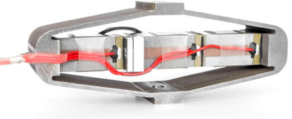
To validate the choice of the APA300ML (Shown in Figure ref:fig:detail_fem_apa300ml_picture):

• the APA300ML is modeled using a Finite Element Software
• a super element is exported and imported in Simscape where its dynamic is studied
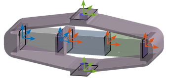
• similarly to what was done with the APA95ML, frames defined for the super element are shown in figure ref:fig:detail_fem_apa300ml_frames

• For this reduced order model, 7 frames are defined and 120 additional modes are modelled for a total matrix size of 162.
• This is very large and will not be practical for simulations, but the best model accuracy was wanted for validation
• The blue frames are used to model the force sensor stack: the relative motion between the two frame is measured
• The red frames are used to model the two actuator stacks: internal force are added
• One mass is fixed at one end of the piezo-electric stack actuator (remove point F), the other end is fixed to the world frame (remote point G).
• The link between mechanical properties and electrical properties was discussed in Section ref:ssec:detail_fem_super_element_validation. As the stacks are the same between the APA300ML and the APA95ML, the values estimated for $g_a$ and $g_s$ are used for the APA300ML.

Identification of the APA Characteristics

Introduction   ignore

A first validation of the FEM and inclusion of the "reduced order flexible model" in the multi body-model is performed by computed some key characteristics of the APA that can be compared against the datasheet.

% Extract the stiffness and mass matrices
K = readmatrix('APA300ML_mat_K.CSV');
M = readmatrix('APA300ML_mat_M.CSV');
[int_xyz, int_i, n_xyz, n_i, nodes] = extractNodes('APA300ML_out_nodes_3D.txt');

Stiffness

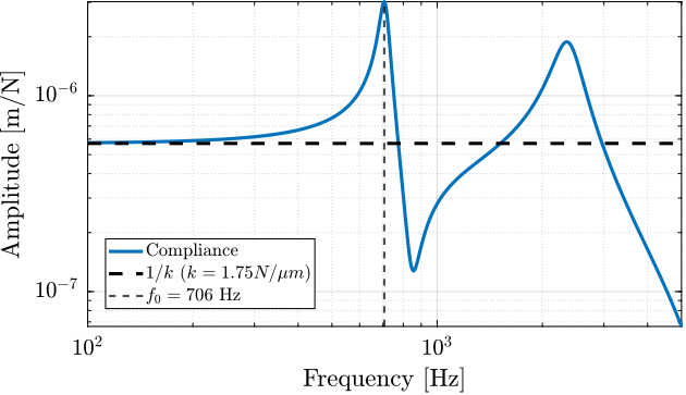
The stiffness is estimated by extracting the transfer function from a vertical force applied on the top frame to the displacement of the same top frame. The inverse of the DC gain this transfer function should be equal to the axial stiffness of the APA300ML. A value of $1.75\,N/\mu m$ is found which is close to the specified stiffness in the datasheet of $k = 1.8\,N/\mu m$. See compliance transfer function ref:fig:detail_fem_apa300ml_compliance.

%% Stiffness estimation
m = 0.0001; % block-free condition, no payload

clear io; io_i = 1;
io(io_i) = linio([mdl, '/Fd'], 1, 'openinput');  io_i = io_i + 1;
io(io_i) = linio([mdl, '/z'],  1, 'openoutput'); io_i = io_i + 1;

G = linearize(mdl, io);

% The inverse of the DC gain of the transfer function
% from vertical force to vertical displacement is the axial stiffness of the APA
k_est = 1/dcgain(G); % [N/m]

Resonance Frequency

The resonance frequency in the block-free condition is specified to be between 650Hz and 840Hz. This is estimated at 709Hz from the model (Figure ref:fig:detail_fem_apa300ml_compliance).

Estimated compliance of the APA300ML

Amplification Factor and Actuator Stroke

The amplification factor is the ratio of the vertical displacement to the (horizontal) stack displacement. It can be estimated from the multi-body model by computing the transfer function from the horizontal motion of the stacks to the vertical motion of the APA. The ratio between the two is found to be equal to $5$. This is linked to the

From the data-sheet of the piezoelectric stacks (see Table ref:tab:detail_fem_stack_parameters, page pageref:tab:detail_fem_stack_parameters), the nominal stroke of the stack is $20\,\mu m$ (which is typical for PZT to have a maximum stroke equal to $0.1\,\%$ of its length, here equal to $20\,mm$). Three stacks are used, for an horizontal stroke of the stacks of $60\,\mu m$. With an amplification factor equal to $5$, the vertical stroke is estimated at $300\,\mu m$, which corresponds to what is indicated in the datasheet.

This analysis provides some confidence on the model accuracy.

Simpler 2DoF Model of the APA300ML

<<sec:apa_model>>

Introduction   ignore

• super-element order is quite large, and therefore not practical for simulations

• the goal here is to develop a low order model, that still represents wanted characteristics of the APA300ML:

  • axial stiffness
  • actuator and force sensor characteristics

• what is not modelled:

  • higher order modes
  • the flexibility of the APA in the other directions
• Therefore this model can be useful for simulations as it contains a very limited number of states, but when more complex dynamics of the APA is to be modelled, a flexible model will be used.

2DoF Model

The model is adapted from cite:souleille18_concep_activ_mount_space_applic.

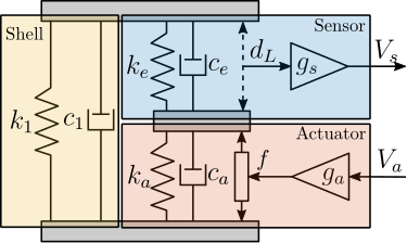
It can be decomposed into three components:

• the shell whose axial properties are represented by $k_1$ and $c_1$
• the actuator stacks whose contribution to the axial stiffness is represented by $k_a$ and $c_a$. The force source $f$ represents the axial force induced by the force sensor stacks. The sensitivity $g_a$ (in $N/m$) is used to convert the applied voltage $V_a$ to the axial force $f$
• the sensor stack whose contribution to the axial stiffness is represented by $k_e$ and $c_e$. A sensor measures the stack strain $d_e$ which is then converted to a voltage $V_s$ using a sensitivity $g_s$ (in $V/m$)

Such a simple model has some limitations:

• it only represents the axial characteristics of the APA as it is modeled as infinitely rigid in the other directions
• some physical insights are lost, such as the amplification factor and the real stress and strain in the piezoelectric stacks
• the creep and hysteresis of the piezoelectric stacks are not modeled as the model is linear

The main advantage is that this model is very simple, only adds 4 states

Schematic of the 2DoF model of the Amplified Piezoelectric Actuator

Parameter Tuning

9 parameters ($m$, $k_1$, $c_1$, $k_e$, $c_e$, $k_a$, $c_a$, $g_s$ and $g_a$) have to be tuned such that the dynamics of the model (Figure ref:fig:detail_fem_apa_2dof_model) well represents the identified dynamics using the FEM.

• Mass is 5kg (similar to the test bench)

• Tune the parameters:

  • From the first zero of the transfer function from Va to Vs, k1 and c1 are tuned
  • From the first pole of the transfer function from Va to y, ka, ca, ke, ce are tuned
  • because the actuator and sensor stacks are physically the same, we suppose Then, it is reasonable to assume that the sensor stacks and the two actuator stacks have identical mechanical characteristics. Therefore, we have $k_e = 2 k_a$ and $c_e = 2 c_a$ as the actuator stack is composed of two stacks in series.
  • In the last step, $g_s$ and $g_a$ for the 2DoF motion can be tuned to match the gain of the transfer functions extracted from the FEM
  • Found parameters are summarized in Table ref:tab:detail_fem_apa300ml_2dof_parameters
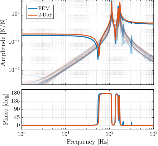
• Comparison of the transfer functions extracted from the high order flexible model with the 4th order (2DoF) model is done in Figure ref:fig:detail_fem_apa300ml_comp_fem_2dof_fem_2dof. Good match is obtained. Of course, higher order modes are not represented by the 2DoF model, nor the limited stiffness in the other directions.

Parameter	Value
$k_1$	$0.30\,N/\mu m$
$k_e$	$4.3\, N/\mu m$
$k_a$	$2.15\,N/\mu m$
$c_1$	$18\,Ns/m$
$c_e$	$0.7\,Ns/m$
$c_a$	$0.35\,Ns/m$
$g_a$	$2.7\,N/V$
$g_s$	$0.53\,V/\mu m$

%% Identify dynamics with "Reduced Order Flexible Body"
m = 5; % [kg]
ga = 25.9; % [N/V]
gs = 5.08e6; % [V/m]

clear io; io_i = 1;
io(io_i) = linio([mdl, '/Va'], 1, 'openinput');  io_i = io_i + 1;
io(io_i) = linio([mdl, '/Fd'], 1, 'openinput');  io_i = io_i + 1;
io(io_i) = linio([mdl, '/z'], 1, 'openoutput'); io_i = io_i + 1;
io(io_i) = linio([mdl, '/Vs'], 1, 'openoutput'); io_i = io_i + 1;

G_fem = linearize(mdl, io);
G_fem_z = G_fem('z','Va');
G_fem_Vs = G_fem('Vs', 'Va');
G_fem_comp = G_fem('z', 'Fd');

%% Determine c1 and k1 from the zero
G_zeros = zero(minreal(G_fem_Vs));
G_zeros = G_zeros(imag(G_zeros)>0);
[~, i_sort] = sort(imag(G_zeros));
G_zeros = G_zeros(i_sort);
G_zero = G_zeros(1);

% Solving 2nd order equations
c1 = -2*m*real(G_zero);
k1 = m*(imag(G_zero)^2 + real(G_zero)^2);

%% Determine ka, ke, ca, ce from the first pole
G_poles = pole(minreal(G_fem_z));
G_poles = G_poles(imag(G_poles)>0);
[~, i_sort] = sort(imag(G_poles));
G_poles = G_poles(i_sort);
G_pole = G_poles(1);

% Solving 2nd order equations
ce = 3*(-2*m*real(G_pole(1)) - c1);
ca = 1/2*ce;

ke = 3*(m*(imag(G_pole)^2 + real(G_pole)^2) - k1);
ka = 1/2*ke;

%% Matching sensor/actuator constants
% ga = dcgain(G_fem_z) / (1/(ka + k1*ke/(k1 + ke)));
clear io; io_i = 1;
io(io_i) = linio([mdl, '_2dof', '/Fa'], 1, 'openinput');  io_i = io_i + 1;
io(io_i) = linio([mdl, '_2dof', '/z'], 1, 'openoutput'); io_i = io_i + 1;
ga = dcgain(G_fem_z)/dcgain(linearize([mdl, '_2dof'], io));

clear io; io_i = 1;
io(io_i) = linio([mdl, '_2dof', '/Va'], 1, 'openinput');  io_i = io_i + 1;
io(io_i) = linio([mdl, '_2dof', '/dL'], 1, 'openoutput'); io_i = io_i + 1;
gs = dcgain(G_fem_Vs)/dcgain(linearize([mdl, '_2dof'], io));

%% Identify dynamics with tuned 2DoF model
clear io; io_i = 1;
io(io_i) = linio([mdl, '_2dof', '/Va'], 1, 'openinput');  io_i = io_i + 1;
io(io_i) = linio([mdl, '_2dof', '/Fd'], 1, 'openinput');  io_i = io_i + 1;
io(io_i) = linio([mdl, '_2dof', '/z'], 1, 'openoutput'); io_i = io_i + 1;
io(io_i) = linio([mdl, '_2dof', '/Vs'], 1, 'openoutput'); io_i = io_i + 1;

G_2dof = linearize([mdl, '_2dof'], io);
G_2dof_z = G_2dof('z','Va');
G_2dof_Vs = G_2dof('Vs', 'Va');
G_2dof_comp = G_2dof('z', 'Fd');

Electrical characteristics of the APA

• Mechanical equations and electrical equations are coupled

• This means for instance, that the stiffness of the piezoelectric stack (i.e. the APA) depends on the electrical boundaries of the stacks:

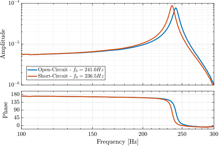
  • Short circuited stacks are less stiff than open-circuited ones
  • This effect is quite small: example with the APA95ML (Figure ref:fig:detail_fem_apa95ml_effect_electrical_boundaries) transfer function from Va to di are estimated with the force sensor stack being short circuited or open-circuited.
• In the model used, the electrical phenomena are not modelled. But as this effect is small, it should be fine
• The electrical characteristics of the APA are very important both from the voltage amplifier side and the ADC measuring the force sensor voltage. This will be discussed in chapter "instrumentation"

%% Effect of electrical boundaries on the
oc = load('detail_fem_apa95ml_open_circuit.mat',  't', 'encoder', 'u');
sc = load('detail_fem_apa95ml_short_circuit.mat', 't', 'encoder', 'u');

% Spectral Analysis parameters
Ts = sc.t(end)/(length(sc.t)-1);
Nfft = floor(2/Ts);
win = hanning(Nfft);
Noverlap = floor(Nfft/2);

% Identification of the transfer function from Va to di
[G_oc,  f]  = tfestimate(detrend(oc.u, 0), detrend(oc.encoder, 0), win, Noverlap, Nfft, 1/Ts);
[G_sc,  f]  = tfestimate(detrend(sc.u, 0), detrend(sc.encoder, 0), win, Noverlap, Nfft, 1/Ts);

% Find resonance frequencies
[~, i_oc] = max(abs(G_oc(f<300)));
[~, i_sc] = max(abs(G_sc(f<300)));

Effect of the electrical bondaries of the force sensor stack on the APA95ML resonance frequency

Validation with the Nano-Hexapod

NASS model + FEM model (or just 2DoF) of APA300ML => validation (based on what?)

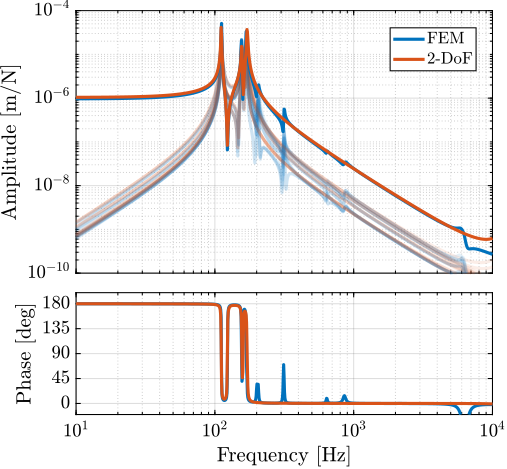
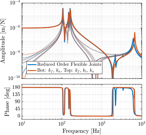
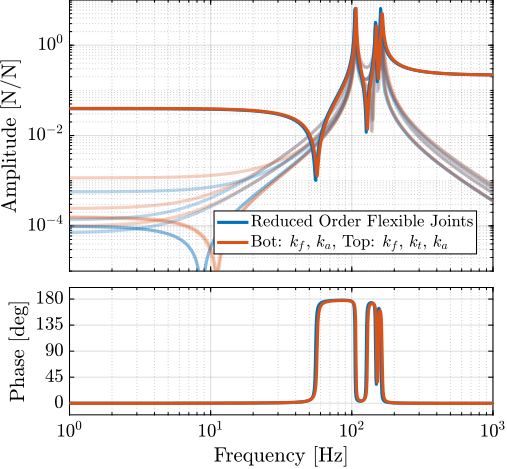
• Compare 2DoF model and FEM (Figure ref:fig:detail_fem_actuator_fem_vs_perfect_plants)

  • HAC plant
  • IFF Plant
  • Very similar => can use 2nd order actuator models

• Talk about model order

  • 2DoF actuators: 24 states
  • FEM actuators: here matrices have a size of 36 36*6+12 => ~300

%% Compare Dynamics between "Reduced Order" flexible joints and "2-dof and 3-dof" joints
% Let's initialize all the stages with default parameters.
initializeGround('type', 'rigid');
initializeGranite('type', 'rigid');
initializeTy('type', 'rigid');
initializeRy('type', 'rigid');
initializeRz('type', 'rigid');
initializeMicroHexapod('type', 'rigid');
initializeSample('m', 50);

initializeSimscapeConfiguration();
initializeDisturbances('enable', false);
initializeLoggingConfiguration('log', 'none');
initializeController('type', 'open-loop');
initializeReferences();

mdl = 'detail_fem_nass';

% Input/Output definition
clear io; io_i = 1;
io(io_i) = linio([mdl, '/Controller'],     1, 'openinput');              io_i = io_i + 1; % Actuator Inputs
io(io_i) = linio([mdl, '/Tracking Error'], 1, 'openoutput', [], 'EdL');  io_i = io_i + 1; % Errors in the frame of the struts
io(io_i) = linio([mdl, '/NASS'],       3, 'openoutput', [], 'fn');  io_i = io_i + 1; % Force Sensors

% Flexible actuators
initializeSimplifiedNanoHexapod('actuator_type', 'flexible', ...
            'flex_type_F', '2dof', ...
            'flex_type_M', '3dof');

G_flex = linearize(mdl, io);
G_flex.InputName  = {'f1', 'f2', 'f3', 'f4', 'f5', 'f6'};
G_flex.OutputName = {'l1', 'l2', 'l3', 'l4', 'l5', 'l6', 'fm1', 'fm2', 'fm3', 'fm4', 'fm5', 'fm6'};

% Actuators modeled as 2DoF system
initializeSimplifiedNanoHexapod('actuator_type', 'apa300ml', ...
            'flex_type_F', '2dof', ...
            'flex_type_M', '3dof');

G_ideal = linearize(mdl, io);
G_ideal.InputName  = {'f1', 'f2', 'f3', 'f4', 'f5', 'f6'};
G_ideal.OutputName = {'l1', 'l2', 'l3', 'l4', 'l5', 'l6', 'fm1', 'fm2', 'fm3', 'fm4', 'fm5', 'fm6'};

Flexible Joint

<<sec:detail_fem_joint>>

Introduction   ignore

The flexible joints have few advantages compared to conventional joints such as the absence of wear, friction and backlash which allows extremely high-precision (predictable) motion. The parasitic bending and torsional stiffness of these joints usually induce some limitation on the control performance. cite:&mcinroy02_model_desig_flexur_joint_stewar

In this document is studied the effect of the mechanical behavior of the flexible joints that are located the extremities of each nano-hexapod's legs.

Ideally, we want the x and y rotations to be free and all the translations to be blocked. However, this is never the case and be have to consider:

• Non-null bending stiffnesses
• Non-null radial compliance
• Axial stiffness in the direction of the legs

This may impose some limitations, also, the goal is to specify the required joints stiffnesses.

Say that for simplicity (reduced number of parts, etc.), we consider the same joints for the fixed based and the top platform.

Outline:

• Perfect flexible joint
• Imperfection of the flexible joint: Model
• Study of the effect of limited stiffness in constrain directions and non-null stiffness in other directions
• Obtained Specification
• Design optimisation (FEM)
• Implementation of flexible elements in the Simscape model: close to simplified model

Flexible joints for Stewart platforms

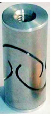
Review of different types of flexible joints for Stewart plaftorms (see Figure ref:fig:detail_fem_joints_examples).

Typical specifications:

• Bending stroke (i.e. long life time by staying away from yield stress, even at maximum deflection/load)
• Axial stiffness
• Bending stiffness
• Maximum axial load
• Well defined rotational axes

Typical values?

• $K_{\theta, \phi} = 15\,[Nm/rad]$ stiffness in flexion
• $K_{\psi} = 20\,[Nm/rad]$ stiffness in torsion
• \[ K_a = 60\,[N/\mu m] \] axial stiffness

Bending and Torsional Stiffness

<<sec:joints_rot_stiffness>>

Because of bending stiffness of the flexible joints, the forces applied by the struts are no longer aligned with the struts (additional forces applied by the "spring force" of the flexible joints).

In this section, we wish to study the effect of the rotation flexibility of the nano-hexapod joints.

• To simplify the analysis, the micro-station is considered rigid, and only the nano-hexapod is considered with:

  • 1dof actuators, k=1N/um, without parallel stiffness to the force sensors
• The bending stiffness of all joints are varied and the dynamics is identified

%% Identify the dynamics for several considered bending stiffnesses
% Let's initialize all the stages with default parameters.
initializeGround('type', 'rigid');
initializeGranite('type', 'rigid');
initializeTy('type', 'rigid');
initializeRy('type', 'rigid');
initializeRz('type', 'rigid');
initializeMicroHexapod('type', 'rigid');
initializeSample('m', 50);

initializeSimscapeConfiguration();
initializeDisturbances('enable', false);
initializeLoggingConfiguration('log', 'none');
initializeController('type', 'open-loop');
initializeReferences();

% Input/Output definition
clear io; io_i = 1;
io(io_i) = linio([mdl, '/Controller'],     1, 'openinput');              io_i = io_i + 1; % Actuator Inputs
io(io_i) = linio([mdl, '/Tracking Error'], 1, 'openoutput', [], 'EdL');  io_i = io_i + 1; % Errors in the frame of the struts
io(io_i) = linio([mdl, '/NASS'],       3, 'openoutput', [], 'fn');  io_i = io_i + 1; % Force Sensors

% Effect of bending stiffness
Kf = [0, 50, 100, 500]; % [Nm/rad]
G_Kf = {zeros(length(Kf), 1)};

for i = 1:length(Kf)
    % Limited joint axial compliance
    initializeSimplifiedNanoHexapod('actuator_type', '1dof', ...
                          'flex_type_F', '2dof', ...
                          'flex_type_M', '3dof', ...
                          'actuator_k', 1e6, ...
                          'actuator_c', 1e1, ...
                          'actuator_kp', 0, ...
                          'actuator_cp', 0, ...
                          'Fsm', 56e-3, ... % APA300ML weight 112g
                          'Msm', 56e-3, ...
                          'Kf_F', Kf(i), ...
                          'Kf_M', Kf(i));

    G_Kf(i) = {linearize(mdl, io)};
    G_Kf{i}.InputName  = {'f1', 'f2', 'f3', 'f4', 'f5', 'f6'};
    G_Kf{i}.OutputName = {'l1', 'l2', 'l3', 'l4', 'l5', 'l6', 'fm1', 'fm2', 'fm3', 'fm4', 'fm5', 'fm6'};
end

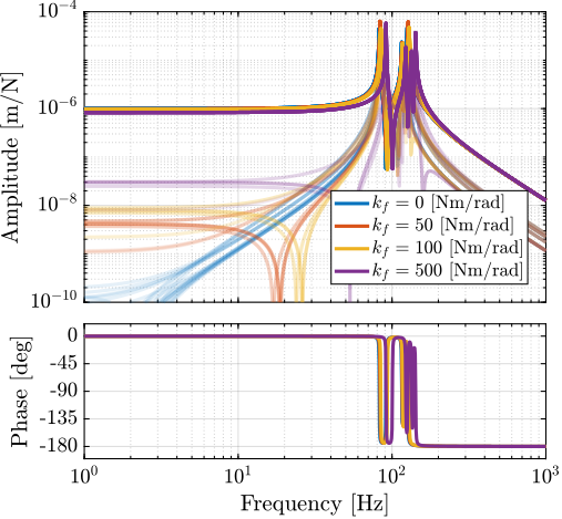
HAC plant (transfer function from f to dL, as measured by the external metrology):

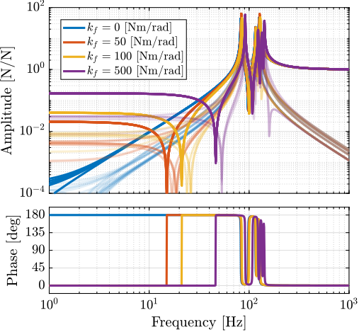
• It increase the coupling at low frequency, but is kept to small values for realistic values of the bending stiffness (Figure ref:fig:detail_fem_joints_bending_stiffness_hac_plant)
• Bending stiffness does not impact significantly the HAC plant. The added stiffness increases the frequency of the suspension modes Condition in cite:&mcinroy02_model_desig_flexur_joint_stewar to have forces aligned with the struts when considering rotational stiffness: kr << k*l^2 For the current nano hexapod configuration, it correspond to << 9000 Nm/rad. This may be an issue for soft nano-hexapod (for instance k = 1e4 => << 90) => have to design very soft flexible joints. Here, having relatively stiff actuators render this condition easier to achieve.

IFF Plant:

• Having bending stiffness adds complex conjugate zero at low frequency (Figure ref:fig:detail_fem_joints_bending_stiffness_iff_plant)
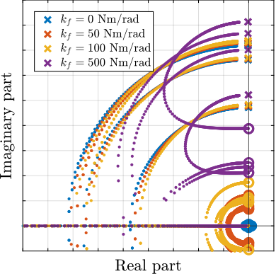
• Similar to having a stiffness in parallel to the struts (i.e., to the force sensor). This can be explained since even if the force sensor is removed (i.e. zero axial stiffness of the strut), the strut will still act as a spring between the mobile and fixed plates because of the bending stiffness of the flexible joints. The frequency of the zero gives an idea of the stiffness contribution of the flexible joint bending stiffness
• They therefore impose limitation for decentralized IFF, as discussed in cite:&preumont07_six_axis_singl_stage_activ
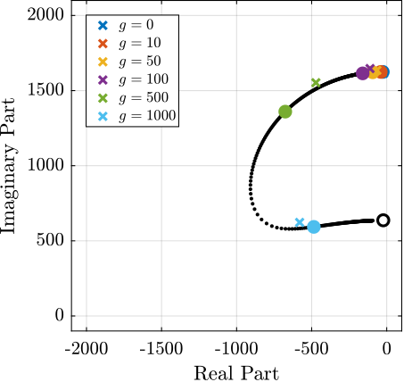
• This can be seen in the root locus plot of Figure ref:fig:detail_fem_joints_bending_stiffness_iff_locus_1dof

However, as the APA300ML was chosen for the actuator, stiffness are already present in parallel to the force sensors:

• The dynamics is computed again for all considered values of the bending stiffnesses with the 2DoF model of the APA300ML
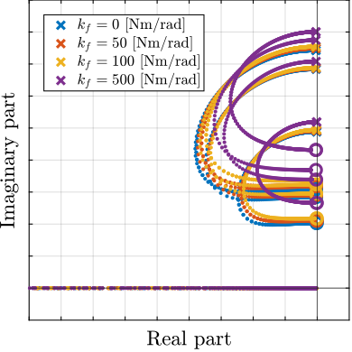
• Root locus for decentralized IFF are shown in Figure ref:fig:detail_fem_joints_bending_stiffness_iff_locus_apa300ml. Now the effect of bending stiffness has little effect on the attainable damping, as its contribution as "parallel stiffness" is small compared to the parallel stiffness already present in the APA300ML.

%% Identify the dynamics for several considered bending stiffnesses - APA300ML
G_Kf_apa300ml = {zeros(length(Kf), 1)};

for i = 1:length(Kf)
    % Limited joint axial compliance
    initializeSimplifiedNanoHexapod('actuator_type', 'apa300ml', ...
                          'flex_type_F', '2dof', ...
                          'flex_type_M', '3dof', ...
                          'Fsm', 56e-3, ... % APA300ML weight 112g
                          'Msm', 56e-3, ...
                          'Kf_F', Kf(i), ...
                          'Kf_M', Kf(i));

    G_Kf_apa300ml(i) = {linearize(mdl, io)};
    G_Kf_apa300ml{i}.InputName  = {'f1', 'f2', 'f3', 'f4', 'f5', 'f6'};
    G_Kf_apa300ml{i}.OutputName = {'l1', 'l2', 'l3', 'l4', 'l5', 'l6', 'fm1', 'fm2', 'fm3', 'fm4', 'fm5', 'fm6'};
end

Conclusion:

• Similar results for torsional stiffness, but less important
• thanks to the use of the APA, the requirements in terms of bending stiffness are less stringent

Axial Stiffness

<<sec:joints_trans_stiffness>>

• Adding flexibility between the actuation point and the measurement point / point of interest is always detrimental for the control performances. This is verified, and the goal is to estimate the minimum axial stiffness that the flexible joints should have
• Here, the mass of the strut should be considered. It is set to 112g as specified in the APA300ML specification sheet.
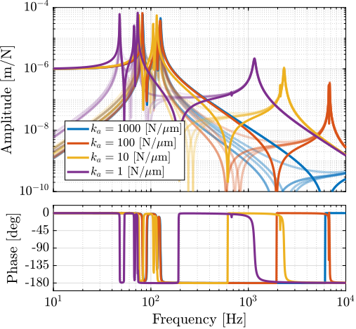
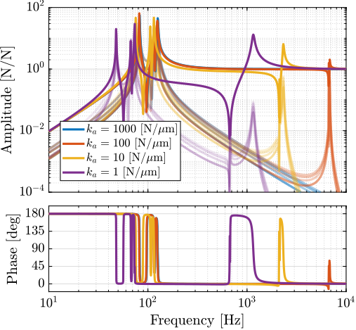
• Transfer functions are estimated for several axial stiffnesses (Figure ref:fig:detail_fem_joints_axial_stiffness_plants)
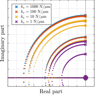
• IFF plant is not much affected (Figure ref:fig:detail_fem_joints_axial_stiffness_iff_plant). Confirmed by the root locus plot of Figure ref:fig:detail_fem_joints_axial_stiffness_iff_locus

• "HAC" plant:

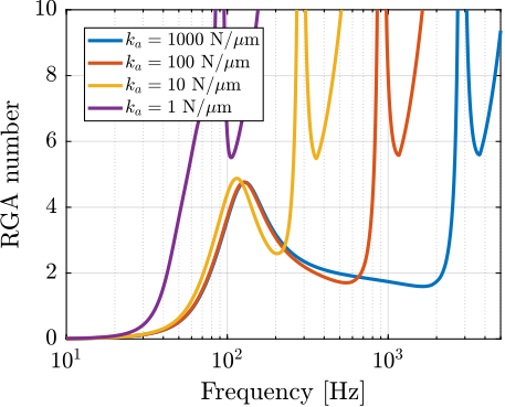
  • Additional modes at high frequency corresponding to internal modes of the struts. It adds coupling to the plant. This is confirmed by computed the RGA-number for the damped plant (i.e. after applying decentralized IFF) in Figure ref:fig:detail_fem_joints_axial_stiffness_rga_hac_plant

%% Identify the dynamics for several considered axial stiffnesses
% Let's initialize all the stages with default parameters.
initializeGround('type', 'rigid');
initializeGranite('type', 'rigid');
initializeTy('type', 'rigid');
initializeRy('type', 'rigid');
initializeRz('type', 'rigid');
initializeMicroHexapod('type', 'rigid');
initializeSample('m', 50);

initializeSimscapeConfiguration();
initializeDisturbances('enable', false);
initializeLoggingConfiguration('log', 'none');
initializeController('type', 'open-loop');
initializeReferences();

% Input/Output definition
clear io; io_i = 1;
io(io_i) = linio([mdl, '/Controller'],     1, 'openinput');              io_i = io_i + 1; % Actuator Inputs
io(io_i) = linio([mdl, '/Tracking Error'], 1, 'openoutput', [], 'EdL');  io_i = io_i + 1; % Errors in the frame of the struts
io(io_i) = linio([mdl, '/NASS'],       3, 'openoutput', [], 'fn');  io_i = io_i + 1; % Force Sensors

% Effect of bending stiffness
Ka = 1e6*[1000, 100, 10, 1]; % [Nm/rad]
G_Ka = {zeros(length(Ka), 1)};

for i = 1:length(Ka)
    % Limited joint axial compliance
    initializeSimplifiedNanoHexapod('actuator_type', '1dof', ...
                          'flex_type_F', '2dof_axial', ...
                          'flex_type_M', '4dof', ...
                          'actuator_k', 1e6, ...
                          'actuator_c', 1e1, ...
                          'actuator_kp', 0, ...
                          'actuator_cp', 0, ...
                          'Fsm', 56e-3, ... % APA300ML weight 112g
                          'Msm', 56e-3, ...
                          'Ca_F', 1, ...
                          'Ca_M', 1, ...
                          'Ka_F', Ka(i), ...
                          'Ka_M', Ka(i));

    G_Ka(i) = {linearize(mdl, io)};
    G_Ka{i}.InputName  = {'f1', 'f2', 'f3', 'f4', 'f5', 'f6'};
    G_Ka{i}.OutputName = {'l1', 'l2', 'l3', 'l4', 'l5', 'l6', 'fm1', 'fm2', 'fm3', 'fm4', 'fm5', 'fm6'};
end

Integral force feedback

• Maybe show the damped plants instead?
• Root Locus: not a lot of effect

%% Compute the damped plants
Kiff = -500 * ...              % Gain
       1/(s + 2*pi*0.1) * ... % LPF: provides integral action
       eye(6);                 % Diagonal 6x6 controller (i.e. decentralized)

Kiff.InputName = {'fm1', 'fm2', 'fm3', 'fm4', 'fm5', 'fm6'};
Kiff.OutputName = {'u1iff', 'u2iff', 'u3iff', 'u4iff', 'u5iff', 'u6iff'};

% New damped plant input
S1 = sumblk("f1 = u1iff + u1");
S2 = sumblk("f2 = u2iff + u2");
S3 = sumblk("f3 = u3iff + u3");
S4 = sumblk("f4 = u4iff + u4");
S5 = sumblk("f5 = u5iff + u5");
S6 = sumblk("f6 = u6iff + u6");

G_Ka_iff = {zeros(1,length(Ka))};
for i=1:length(Ka)
    G_Ka_iff(i) = {connect(G_Ka{i}, Kiff, S1, S2, S3, S4, S5, S6, {'u1', 'u2', 'u3', 'u4', 'u5', 'u6'}, {'l1', 'l2', 'l3', 'l4', 'l5', 'l6'})};
end

%% Interaction Analysis - RGA Number
rga = zeros(length(Ka), length(freqs));
for i = 1:length(Ka)
    for j = 1:length(freqs)
        rga(i,j) = sum(sum(abs(inv(evalfr(G_Ka_iff{i}({"l1", "l2", "l3", "l4", "l5", "l6"}, {"u1", "u2", "u3", "u4", "u5", "u6"}), 1j*2*pi*freqs(j)).').*evalfr(G_Ka_iff{i}({"l1", "l2", "l3", "l4", "l5", "l6"}, {"u1", "u2", "u3", "u4", "u5", "u6"}), 1j*2*pi*freqs(j)) - eye(6))));
    end
end

Conclusion:

• The axial stiffness of the flexible joints should be maximized to limit additional coupling at high frequency that may negatively impact the achievable bandwidth
• It should be much higher than the stiffness of the actuator
• For the nano-hexapod 100N/um is a reasonable axial stiffness specification
• Above the resonance frequency linked to the limited axial stiffness of the flexible joint, the system becomes coupled and impossible to control
• Also, loose control authority at the frequency of the zero

Obtained design / Specifications

• Summary of specifications (Table ref:tab:detail_fem_joints_specs)

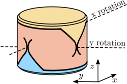
• Explain choice of geometry:

  • x and y rotations are coincident
  • stiffness can be easily tuned
  • high axial stiffness

• Explain how it is optimized:

  • Extract stiffnesses from FEM
  • Parameterized model in the FE software

  • Quick optimization: (few iterations, could probably increase more the axial stiffness)

    • There is a trade off between high axial stiffness and low bending/torsion stiffness
    • Also check the yield strength

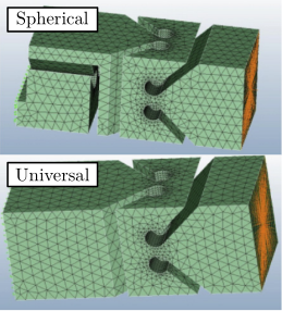
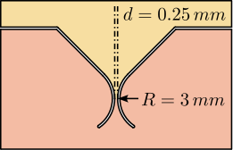
• Show obtained geometry Figure ref:fig:detail_fem_joints_design:

  • "neck" size: 0.25mm
• Characteristics of the flexible joints obtained from FEA are summarized in Table ref:tab:detail_fem_joints_specs

	Specification	FEM
Axial Stiffness $k_a$	$> 100\,N/\mu m$	94
Shear Stiffness $k_s$	$> 1\,N/\mu m$	13
Bending Stiffness $k_f$	$< 100\,Nm/\text{rad}$	5
Torsion Stiffness $k_t$	$< 500\,Nm/\text{rad}$	260
Bending Stroke	$> 1\,\text{mrad}$	24.5

Validation with the Nano-Hexapod

To validate the designed flexible joint:

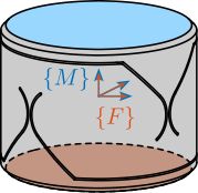
• FEM: modal reduction two interface frames are defined (Figure ref:fig:detail_fem_joints_frames)
• additional 6 modes are extracted: size of reduced order mass and stiffness matrices: $18 \times 18$
• Imported in the multi-body model
• The transfer functions from forces and torques applied between frames $\{F\}$ and $\{M\}$ to the relative displacement/rotations of the two frames is extracted.
• The stiffness characteristics of the flexible joint is estimated from the low frequency gain of the obtained transfer functions. Same values are obtained with the reduced order model and the FEM.

Defined frames for the reduced order flexible body. The two flat interfaces are considered rigid, and are linked to the two frames $\{F\}$ and $\{M\}$ both located at the center of the rotation.

%% Extract stiffness of the joint from the reduced order model
% We first extract the stiffness and mass matrices.
K = readmatrix('flex025_mat_K.CSV');
M = readmatrix('flex025_mat_M.CSV');
% Then, we extract the coordinates of the interface nodes.
[int_xyz, int_i, n_xyz, n_i, nodes] = extractNodes('flex025_out_nodes_3D.txt');

m = 1;

%% Name of the Simulink File
mdl = 'detail_fem_joint';

%% Input/Output definition
clear io; io_i = 1;
io(io_i) = linio([mdl, '/T'], 1, 'openinput');  io_i = io_i + 1; % Forces and Torques
io(io_i) = linio([mdl, '/D'], 1, 'openoutput'); io_i = io_i + 1; % Translations and Rotations

G = linearize(mdl, io);

% Stiffness extracted from the Simscape model
k_a = 1/dcgain(G(3,3)); % Axial stiffness [N/m]
k_f = 1/dcgain(G(4,4)); % Bending stiffness [N/m]
k_t = 1/dcgain(G(6,6)); % Torsion stiffness [N/m]


% Stiffness extracted from the Stiffness matrix
k_s = K(1,1); % shear [N/m]
% k_s = K(2,2); % shear [N/m]
k_a = K(3,3); % axial [N/m]
k_f = K(4,4); % bending [Nm/rad]
% k_f = K(5,5); % bending [Nm/rad]
k_t =  K(6,6); % torsion [Nm/rad]

Depending on which characteristic of the flexible joint is to be modelled, several DoFs can be taken into account:

• 2DoF (universal joint) $k_f$
• 3DoF (spherical joint) taking into account torsion $k_f$, $k_t$
• 2DoF + axial stiffness $k_f$, $k_a$
• 3DoF + axial stiffness $k_f$, $k_t$, $k_a$
• 6DoF ("bushing joint") $k_f$, $k_t$, $k_a$, $k_s$

Adding more degrees of freedom:

• can represent important features
• adds model states that may not be relevant for the dynamics, and may complexity the simulations without adding much information

After testing different configurations, a good compromise was found for the modelling of the nano-hexapod flexible joints:

• bottom joints: $k_f$ and $k_a$
• top joints: $k_f$, $k_t$ and $k_a$

Talk about model order:

• with flexible joints: 252 states:

  • 12 for the payload (6 dof)
  • 12 for the 2DoF struts
  • 216 DoF for the flexible joints (18*6*2)
  • 12 states for?

• with 3dof and 4dof: 48 states

  • 12 for the payload (6 dof)
  • 12 for the 2DoF struts
  • 12 states for the bottom joints
  • 12 states for the top joints

%% Compare Dynamics between "Reduced Order" flexible joints and "2-dof and 3-dof" joints
% Let's initialize all the stages with default parameters.
initializeGround('type', 'rigid');
initializeGranite('type', 'rigid');
initializeTy('type', 'rigid');
initializeRy('type', 'rigid');
initializeRz('type', 'rigid');
initializeMicroHexapod('type', 'rigid');
initializeSample('m', 50);

initializeSimscapeConfiguration();
initializeDisturbances('enable', false);
initializeLoggingConfiguration('log', 'none');
initializeController('type', 'open-loop');
initializeReferences();

mdl = 'detail_fem_nass';

% Input/Output definition
clear io; io_i = 1;
io(io_i) = linio([mdl, '/Controller'],     1, 'openinput');              io_i = io_i + 1; % Actuator Inputs
io(io_i) = linio([mdl, '/Tracking Error'], 1, 'openoutput', [], 'EdL');  io_i = io_i + 1; % Errors in the frame of the struts
io(io_i) = linio([mdl, '/NASS'],       3, 'openoutput', [], 'fn');  io_i = io_i + 1; % Force Sensors

% Fully flexible joints
initializeSimplifiedNanoHexapod('actuator_type', 'apa300ml', ...
            'flex_type_F', 'flexible', ...
            'flex_type_M', 'flexible', ...
            'Fsm', 56e-3, ... % APA300ML weight 112g
            'Msm', 56e-3);

G_flex = linearize(mdl, io);
G_flex.InputName  = {'f1', 'f2', 'f3', 'f4', 'f5', 'f6'};
G_flex.OutputName = {'l1', 'l2', 'l3', 'l4', 'l5', 'l6', 'fm1', 'fm2', 'fm3', 'fm4', 'fm5', 'fm6'};

% Flexible joints modelled by 2DoF and 3DoF joints
initializeSimplifiedNanoHexapod('actuator_type', 'apa300ml', ...
            'flex_type_F', '2dof_axial', ...
            'flex_type_M', '4dof', ...
            'Kf_F', k_f, ...
            'Kt_F', k_t, ...
            'Ka_F', k_a, ...
            'Kf_M', k_f, ...
            'Kt_M', k_t, ...
            'Ka_M', k_a, ...
            'Cf_F', 1e-2, ...
            'Ct_F', 1e-2, ...
            'Ca_F', 1e-2, ...
            'Cf_M', 1e-2, ...
            'Ct_M', 1e-2, ...
            'Ca_M', 1e-2, ...
            'Fsm', 56e-3, ... % APA300ML weight 112g
            'Msm', 56e-3);

G_ideal = linearize(mdl, io);
G_ideal.InputName  = {'f1', 'f2', 'f3', 'f4', 'f5', 'f6'};
G_ideal.OutputName = {'l1', 'l2', 'l3', 'l4', 'l5', 'l6', 'fm1', 'fm2', 'fm3', 'fm4', 'fm5', 'fm6'};

Conclusion

<<sec:detail_fem_conclusion>>

Bibliography   ignore

Footnotes

¹The manufacturer of the APA95ML was not willing to share the piezoelectric material properties of the stack.

---