phd-micro-station-modal-analysis/modal-analysis.org

Micro-Station - Modal Analysis

• Introduction
• Measurement Setup
  • Introduction
  • Used Instrumentation
  • Structure Preparation and Test Planing
  • Location of the Accelerometers
  • Hammer Impacts
  • Force and Response signals
• Frequency Analysis
  • Introduction
  • First verification of the solid body assumption
  • From accelerometer DOFs to solid body DOFs
  • Frequency Response Matrix expressed at the Center of Mass
    • What reference frame to choose?
    • Center of Mass of each solid body
    • Computation
  • Verify that we find the original FRF from the FRF in the global coordinates
• Modal Analysis
  • Introduction
  • Determine the number of modes
    • Singular Value Decomposition - Modal Indication Function
    • Composite Response Function
  • Modal parameter extraction
    • OROS - Modal software
    • Importation of the modal parameters on Matlab
    • Theory
    • Modal Matrices
  • Obtained Mode Shapes animations
  • Verify the validity of the Modal Model
• Conclusion
• Bibliography

---

This report is also available as a pdf.

---

Introduction   ignore

In order to properly make a multi-body model of the micro-station, an experimental modal-analysis is performed.

In fact, even though it is easy to estimate the inertia of each solid body from its geometry and its material density, it is much more difficult to properly estimate the stiffness and damping properties of the guiding elements connecting each solid body.

In this report, an experimental modal analysis is perform in order to ease the development of the multi-body model.

The measurement setup used for modal analysis is presented in Section ref:sec:modal_meas_setup. This includes the instrumentation used (i.e. instrumented hammer, accelerometers and acquisition system), the test planing, and the first analysis of the obtained signals.

In Section ref:sec:modal_frf_processing, the obtained frequency response functions between the forces applied using the instrumented hammer and the various accelerometers fixed to the structure are computed. These measurements are then projected at the center of mass of each solid body to ease the further use of the results. The solid body assumption is also validated.

Finally, the modal analysis is performed in Section ref:sec:modal_analysis.

cite:&ewins00_modal

Sections	Matlab File
Section ref:sec:modal_meas_setup	modal_1_meas_setup.m
Section ref:sec:modal_frf_processing	modal_2_frf_processing.m
Section ref:sec:modal_analysis	modal_3_analysis.m

Measurement Setup

<<sec:modal_meas_setup>>

Introduction   ignore

ref:ssec:modal_instrumentation ref:ssec:modal_test_preparation ref:ssec:modal_accelerometers ref:ssec:modal_hammer_impacts ref:ssec:modal_measured_signals

Used Instrumentation

<<ssec:modal_instrumentation>> In order to perform to Modal Analysis and to obtain first a Response Model, the following devices are used:

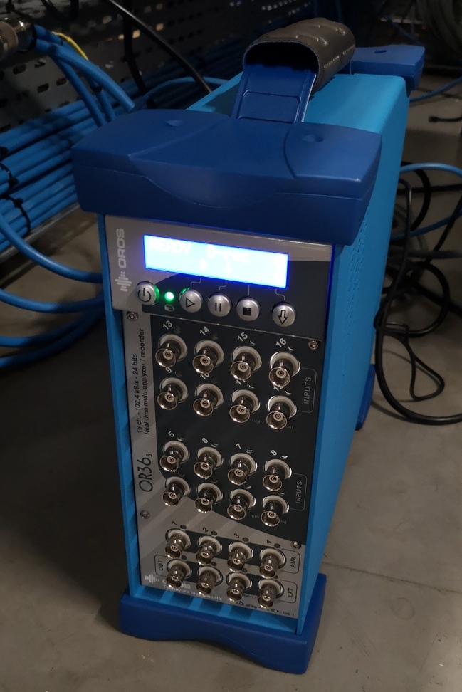
• An acquisition system (OROS) with 24bits ADCs (figure ref:fig:modal_oros)
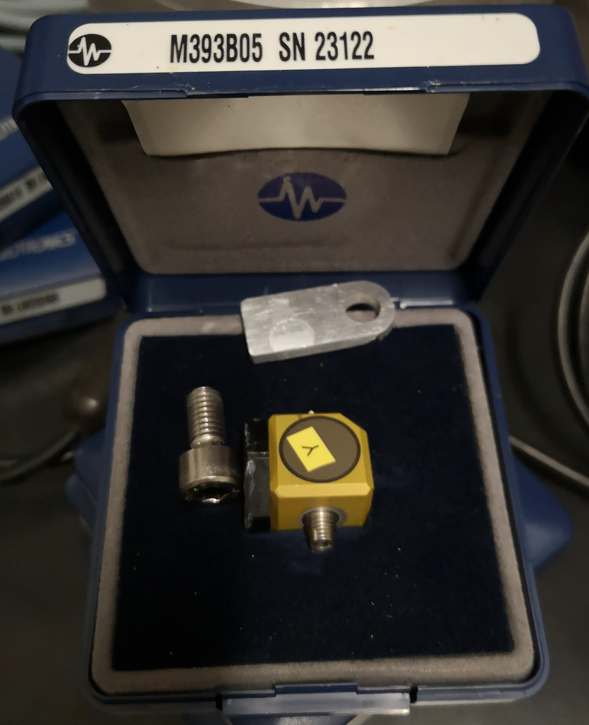
• 3 tri-axis Accelerometers (figure ref:fig:modal_accelero_M393B05) with parameters shown on table ref:tab:modal_accelero_M393B05
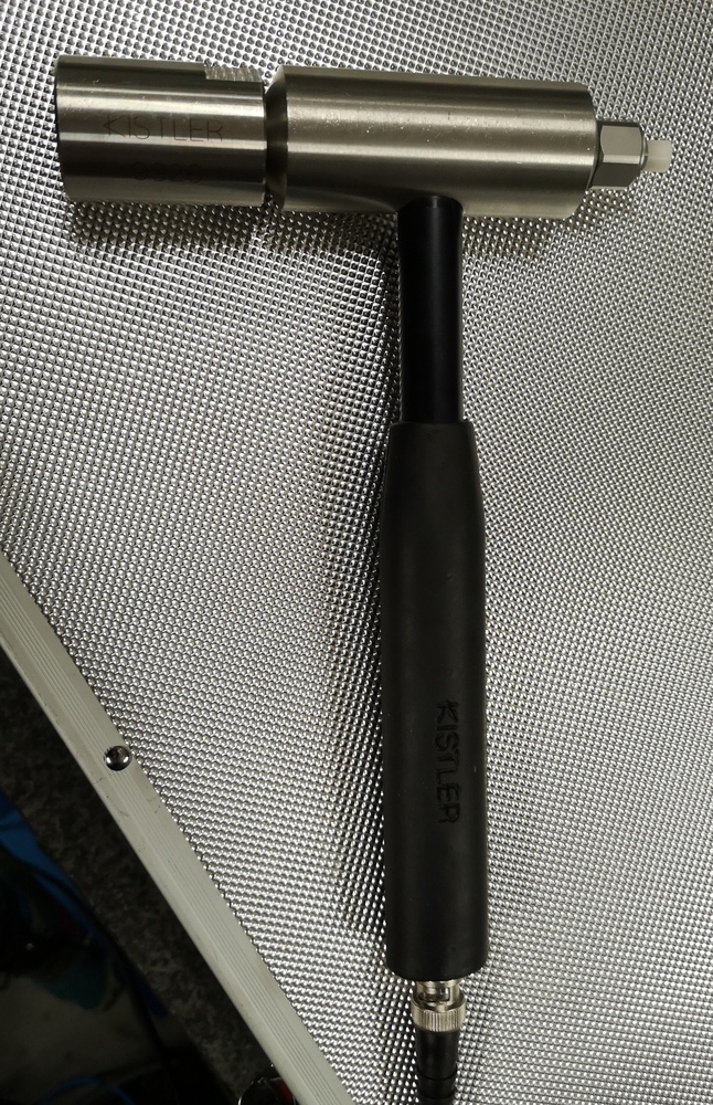
• An Instrumented Hammer with various Tips (figure ref:fig:modal_instrumented_hammer)

Instrumentation used for the modal analysis

The acquisition system permits to auto-range the inputs (probably using variable gain amplifiers) the obtain the maximum dynamic range. This is done before each measurement. Anti-aliasing filters are also included in the system.

Sensitivity	$10\,V/g$
Measurement Range	0.5 g pk
Broadband Resolution	$\SI{4}{\micro\g\rms}$
Frequency Range	$0.7$ to $\SI{450}{Hz}$
Resonance Frequency	$> \SI{2.5}{kHz}$

Tests have been conducted to determine the most suitable Hammer tip. This has been found that the softer tip gives the best results. It excites more the low frequency range where the coherence is low, the overall coherence was improved.

The accelerometers are glued on the structure.

Structure Preparation and Test Planing

<<ssec:modal_test_preparation>> All the stages are turned ON. This is done for two reasons:

• Be closer to the real dynamic of the station in used
• If the control system of stages are turned OFF, this would results in very low frequency modes un-identifiable with the current setup, and this will also decouple the dynamics which would not be the case in practice

This is critical for the translation stage and the spindle as their is no stiffness in the free DOF (air-bearing for the spindle for instance).

The alternative would have been to mechanically block the stages with screws, but this may result in changing the modes.

The stages turned ON are:

• Translation Stage
• Tilt Stage
• Spindle and Slip-Ring
• Hexapod

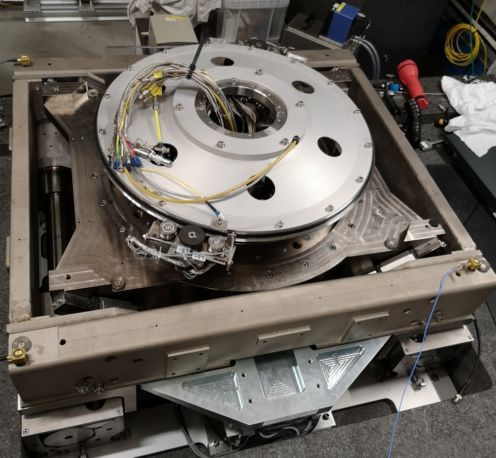
The top part representing the NASS and the sample platform have been removed in order to reduce the complexity of the dynamics and also because this will be further added in the model inside Simscape.

All the stages are moved to their zero position (Ty, Ry, Rz, Slip-Ring, Hexapod).

All other elements have been remove from the granite such as another heavy positioning system.

The goal is to identify the full $N \times N$ FRF matrix $H$ (where $N$ is the number of degree of freedom of the system):

\begin{equation} H_{jk} = \frac{X_j}{F_k} \end{equation}

However, from only one column or one line of the matrix, we can compute the other terms thanks to the principle of reciprocity.

Either we choose to identify $\frac{X_k}{F_i}$ or $\frac{X_i}{F_k}$ for any chosen $k$ and for $i = 1,\ ...,\ N$.

We here choose to identify $\frac{X_i}{F_k}$ for practical reasons:

• it is easier to glue the accelerometers on all the stages and excite only a one particular point than doing the opposite

The measurement thus consists of:

• always excite the structure at the same location with the Hammer
• Move the accelerometers to measure all the DOF of the structure

We will measured 3 columns (3 impacts location) in order to have some redundancy and to make sure that all modes are excited.

Location of the Accelerometers

<<ssec:modal_accelerometers>> 4 tri-axis accelerometers are used for each solid body.

Only 2 could have been used as only 6DOF have to be measured, however, we have chosen to have some redundancy.

This could also help us identify measurement problems or flexible modes is present.

The position of the accelerometers are:

• 4 on the first granite
• 4 on the second granite
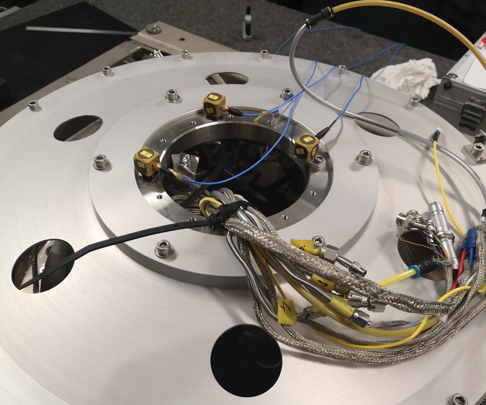
• 4 on top of the translation stage (figure ref:fig:modal_accelerometers_ty)
• 4 on top of the tilt stage
• 3 on top of the spindle
• 4 on top of the hexapod (figure ref:fig:modal_accelerometers_hexapod)

In total, 23 accelerometers are used: 69 DOFs are thus measured.

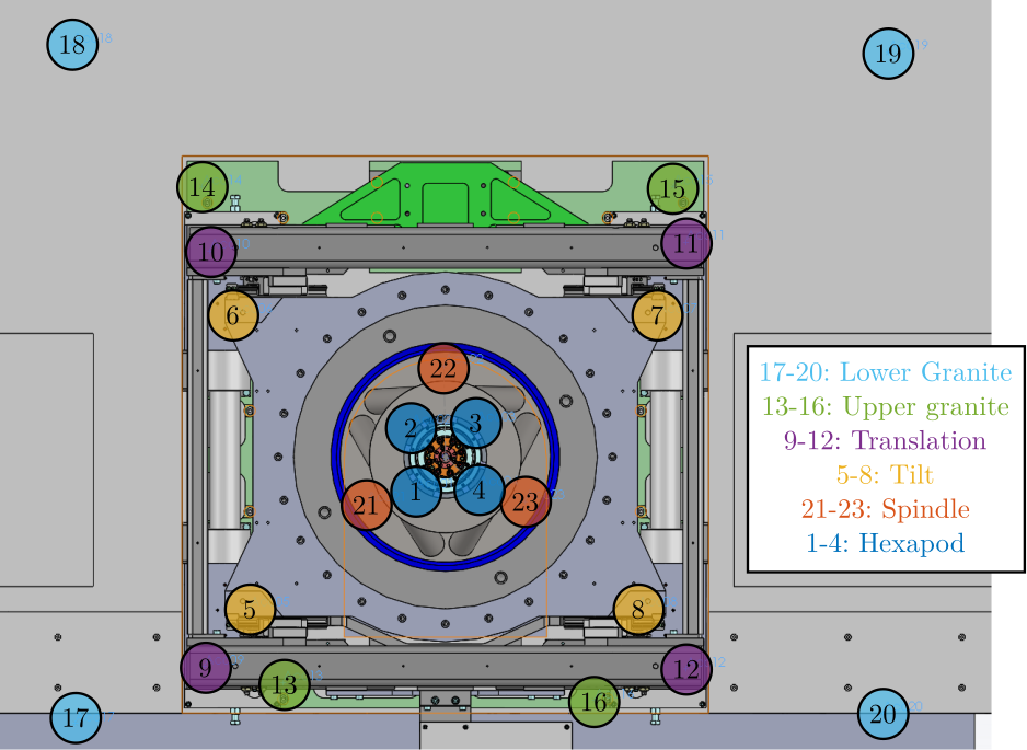
The precise determination of the position of each accelerometer is done using the SolidWorks model (shown on figure ref:fig:modal_location_accelerometers).

Accelerometers fixed on the micro-station

The precise position of all the 23 accelerometer with respect to a frame located at the point of interest (located 270mm above the top platform of the hexapod) are shown in table ref:tab:modal_position_accelerometers.

%% Load Accelerometer positions
acc_pos = readtable('mat/acc_pos.txt', 'ReadVariableNames', false);
acc_pos = table2array(acc_pos(:, 1:4));
[~, i] = sort(acc_pos(:, 1));
acc_pos = acc_pos(i, 2:4);

	ID	$x$ [mm]	$y$ [mm]	$z$ [mm]
Hexapod	1	-64	-64	-270
Hexapod	2	-64	64	-270
Hexapod	3	64	64	-270
Hexapod	4	64	-64	-270
Tilt	5	-385	-300	-417
Tilt	6	-420	280	-417
Tilt	7	420	280	-417
Tilt	8	380	-300	-417
Translation	9	-475	-414	-427
Translation	10	-465	407	-427
Translation	11	475	424	-427
Translation	12	475	-419	-427
Upper Granite	13	-320	-446	-786
Upper Granite	14	-480	534	-786
Upper Granite	15	450	534	-786
Upper Granite	16	295	-481	-786
Lower Granite	17	-730	-526	-951
Lower Granite	18	-735	814	-951
Lower Granite	19	875	799	-951
Lower Granite	20	865	-506	-951
Spindle	21	-155	-90	-594
Spindle	22	0	180	-594
Spindle	23	155	-90	-594

Hammer Impacts

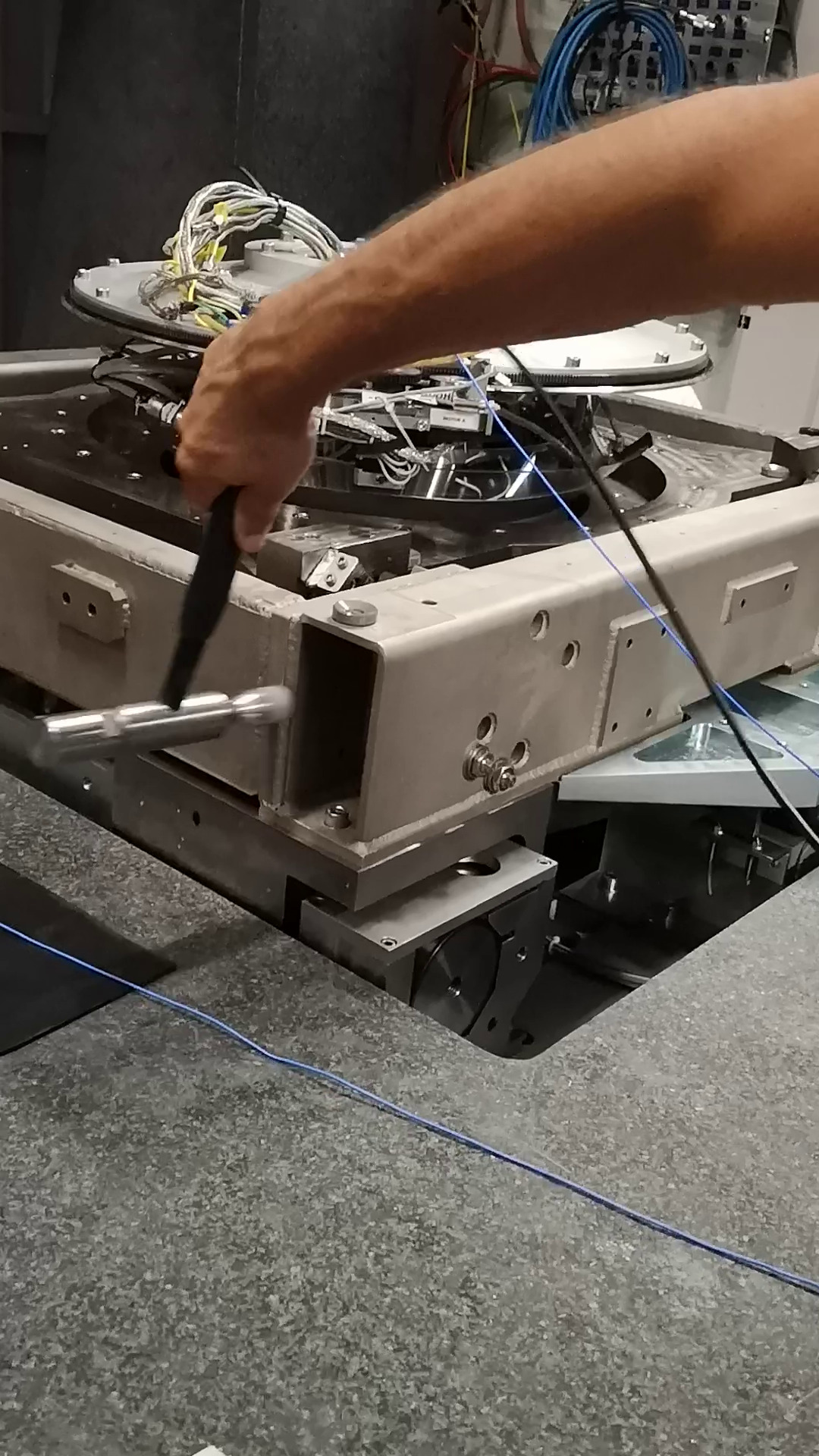
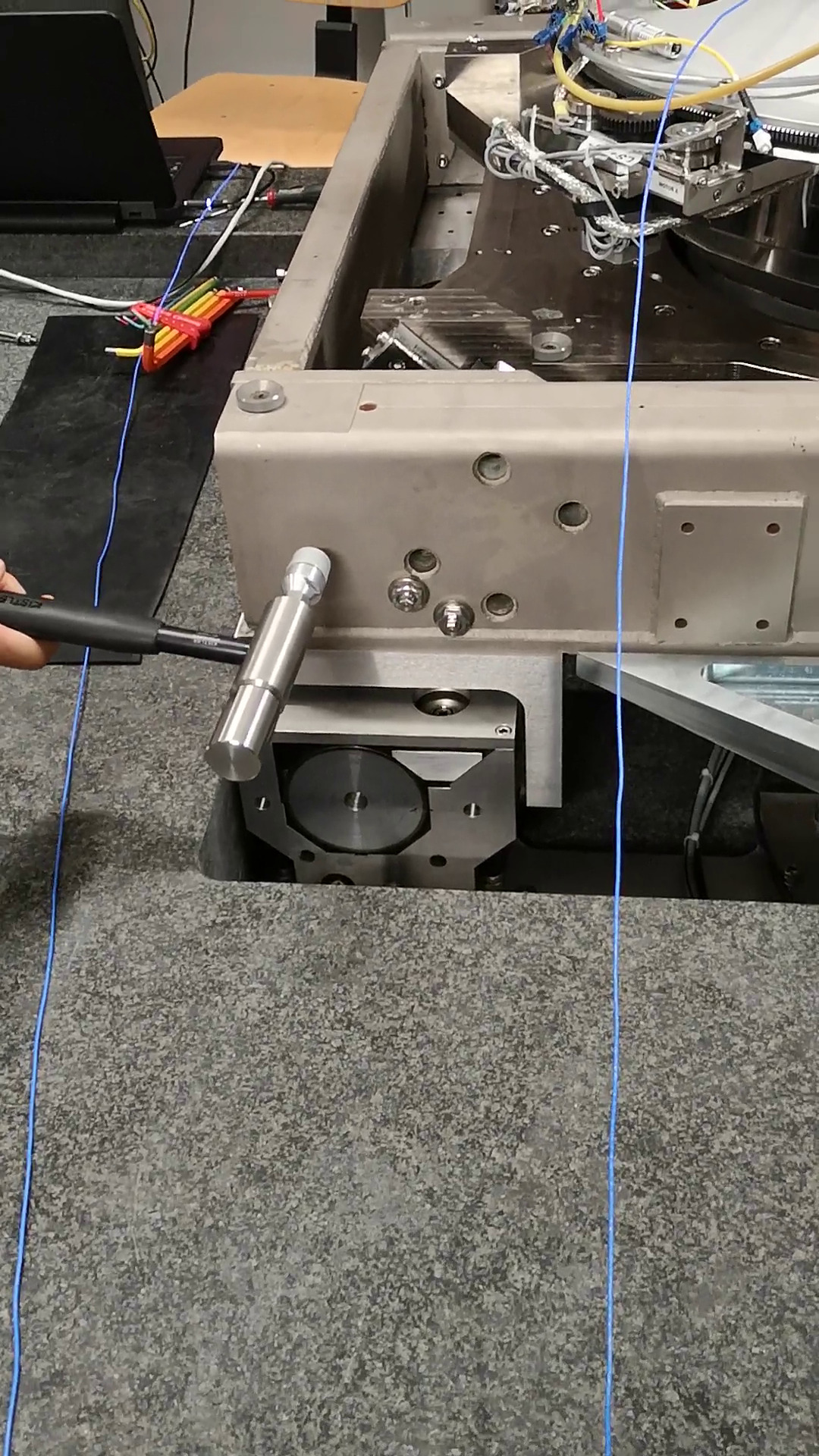
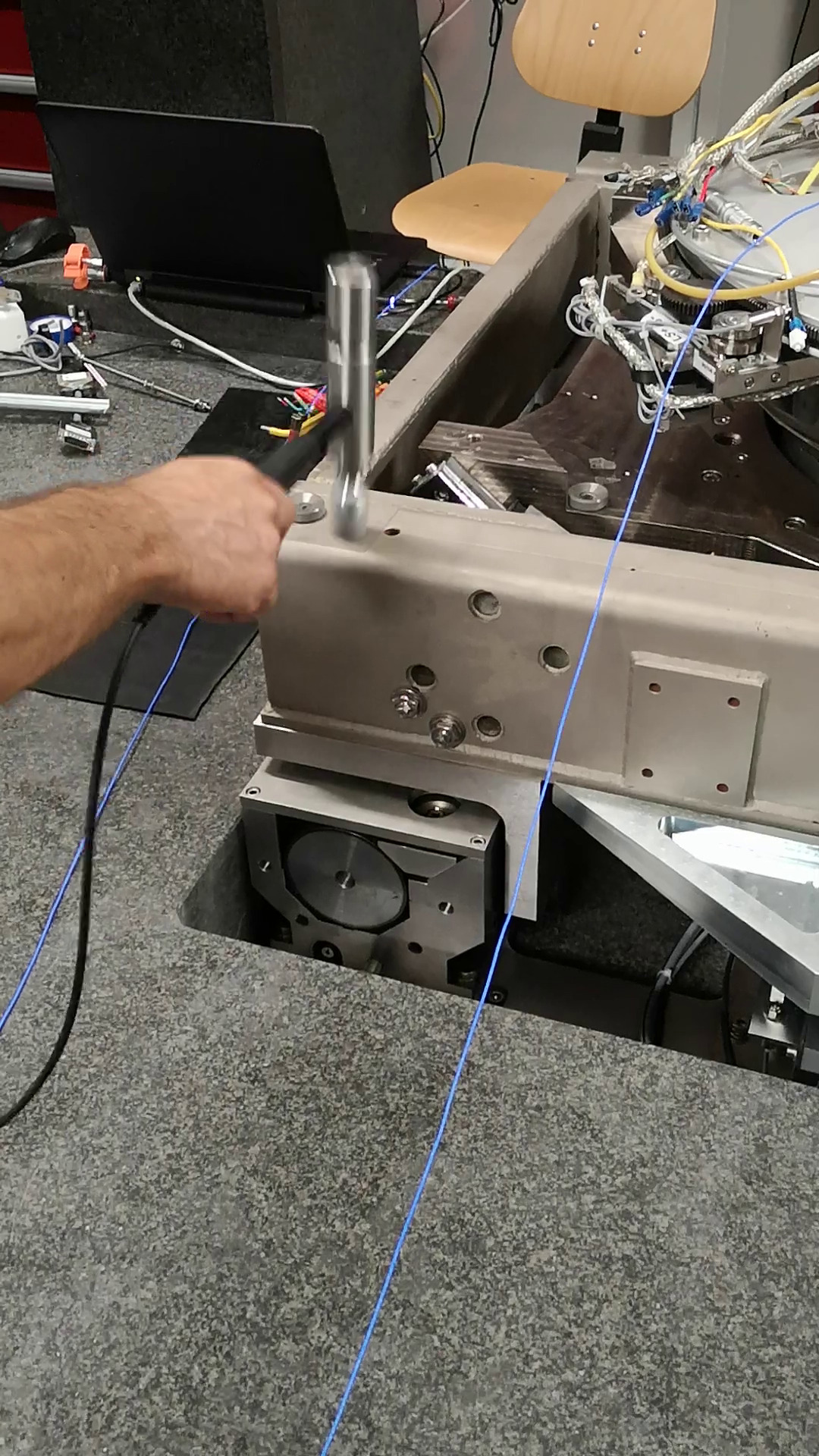
<<ssec:modal_hammer_impacts>> Only 3 impact points are used. The impact points are shown on figures ref:fig:modal_impact_x, ref:fig:modal_impact_y and ref:fig:modal_impact_z.

We chose this excitation point as it seems to excite all the modes in the frequency band of interest and because it provides good coherence for all the accelerometers.

From cite:ewins00_modal: Most modal test require a point mobility measurement as one of the measured FRF. This is hard to achieve as both force and response transducer should be at the same point on the structure.

The three hammer impacts used for the modal analysis

Force and Response signals

<<ssec:modal_measured_signals>>

%% Load raw data
meas1_raw = load('mat/meas_raw_1.mat');

% Sampling Frequency [Hz]
Fs = 1/meas1_raw.Track1_X_Resolution;

% Time just before the impact occurs [s]
impacts = [5.937, 11.228, 16.681, 22.205, 27.350, 32.714, 38.115, 43.888, 50.407]-0.01;

% Time vector [s]
time = linspace(0, meas1_raw.Track1_X_Resolution*length(meas1_raw.Track1), length(meas1_raw.Track1));

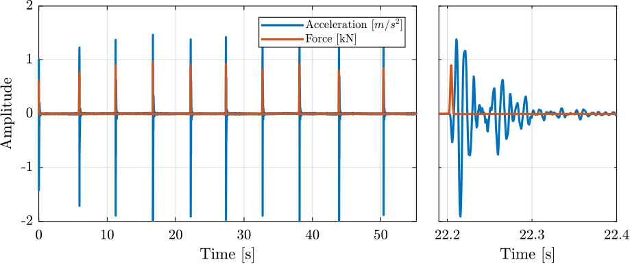
The force sensor and the accelerometers signals are shown in the time domain in Figure ref:fig:modal_raw_meas. Sharp "impacts" can be seen for the force sensor, indicating wide frequency band excitation. For the accelerometer, many resonances can be seen on the right, indicating complex dynamics

Raw measurement of the acceleromter (blue) and of the force sensor at the Hammer tip (red). Zoom on one impact is shown on the right.

%% Frequency Analysis
Nfft = floor(5.0*Fs); % Number of frequency points
win = hanning(Nfft); % Windowing
Noverlap = floor(Nfft/2); % Overlap for frequency analysis

%% Comnpute the power spectral density of the force and acceleration
[pxx_force, f] = pwelch(meas1_raw.Track1, win, Noverlap, Nfft, Fs);
[pxx_acc,   ~] = pwelch(meas1_raw.Track2, win, Noverlap, Nfft, Fs);

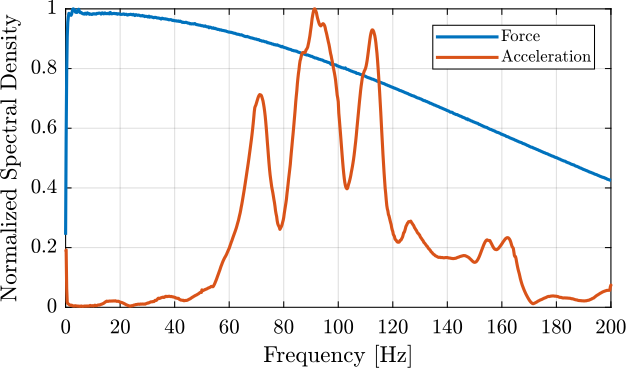
The "normalized" amplitude spectral density of the two signals are computed and shown in Figure ref:fig:modal_asd_acc_force. Conclusions based on the time domain signals can be clearly seen in the frequency domain (wide frequency content for the force signal and complex dynamics for the accelerometer).

Normalized Amplitude Spectral Density of the measured force and acceleration

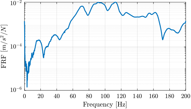
The frequency response function from the applied force to the measured acceleration can then be computed (Figure ref:fig:modal_frf_acc_force).

%% Compute the transfer function and Coherence
[G1,   f] = tfestimate(meas1_raw.Track1, meas1_raw.Track2, win, Noverlap, Nfft, Fs);
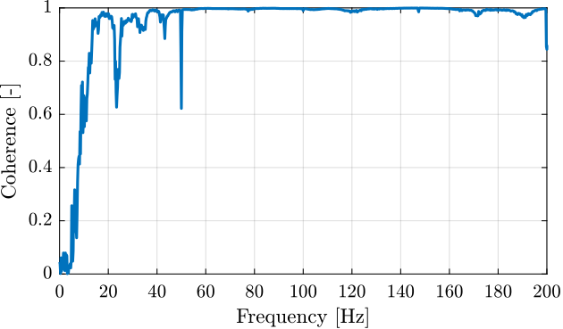
[coh1, ~] = mscohere(  meas1_raw.Track1, meas1_raw.Track2, win, Noverlap, Nfft, Fs);

Frequency Response Function between the measured force and acceleration

The coherence between the input and output signals is also computed and found to be good between 20 and 200Hz (Figure ref:fig:modal_coh_acc_force).

Coherence between the measured force and acceleration

Frequency Analysis

<<sec:modal_frf_processing>>

Introduction   ignore

The measurements have been conducted and a $n \times p \times q$ Frequency Response Functions Matrix has been computed with:

• $n$: the number of output measured accelerations: $23 \times 3 = 69$ (23 accelerometers measuring 3 directions each)
• $p$: the number of input force excitations: $3$
• $q$: the number of frequency points $\omega_i$

Thus, the FRF matrix is an $69 \times 3 \times 801$ matrix.

For each frequency point $\omega_i$, a 2D matrix is obtained that links the 3 force inputs to the 69 output accelerations:

\begin{equation} \text{FRF}(\omega_i) = \begin{bmatrix} \frac{D_{1_x}}{F_x}(\omega_i) & \frac{D_{1_x}}{F_y}(\omega_i) & \frac{D_{1_x}}{F_z}(\omega_i) \\ \frac{D_{1_y}}{F_x}(\omega_i) & \frac{D_{1_y}}{F_y}(\omega_i) & \frac{D_{1_y}}{F_z}(\omega_i) \\ \frac{D_{1_z}}{F_x}(\omega_i) & \frac{D_{1_z}}{F_y}(\omega_i) & \frac{D_{1_z}}{F_z}(\omega_i) \\ \frac{D_{2_x}}{F_x}(\omega_i) & \frac{D_{2_x}}{F_y}(\omega_i) & \frac{D_{2_x}}{F_z}(\omega_i) \\ \vdots & \vdots & \vdots \\ \frac{D_{23_z}}{F_x}(\omega_i) & \frac{D_{23_z}}{F_y}(\omega_i) & \frac{D_{23_z}}{F_z}(\omega_i) \\ \end{bmatrix} \end{equation}

However, for the multi-body model being developed, only 6 solid bodies are considered, namely: the bottom granite, the top granite, the translation stage, the tilt stage, the spindle and the hexapod. Therefore, only $6 \times 6 = 36$ degrees of freedom are of interest.

The objective in this section is therefore to process the Frequency Response Matrix to reduce the number of measured DoFs from 69 to 36.

In order to be able to perform this reduction of measured DoFs, the measures stages have to behave as rigid bodies in the frequency band of interest. This

ref:ssec:modal_solid_body_first_check

To go from the accelerometers DoFs to the solid body 6 DoFs (three translations and three rotations), some computations have to be performed. This is explained in Section ref:ssec:modal_acc_to_solid_dof.

Finally, the $69 \times 3 \times 801$ frequency response matrix is reduced to a $36 \times 3 \times 801$ frequency response matrix where the motion of each solid body is expressed with respect to the CoM of the solid body (Section ref:ssec:modal_frf_com).

To validate this reduction of DoF and the solid body assumption, the frequency response function at the accelerometer location are synthesized from the reduced frequency response matrix and are compared with the initial measurements in Section ref:ssec:modal_solid_body_assumption.

First verification of the solid body assumption

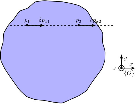
<<ssec:modal_solid_body_first_check>> In this section, it is shown that two accelerometers fixed to a rigid body at positions $\vec{p}_1$ and $\vec{p}_2$ in such a way that $\vec{p}_2 = \vec{p}_1 + \alpha \vec{x}$ will measure the same value in the $\vec{x}$ direction. Such situation is illustrated on Figure ref:fig:modal_aligned_accelerometers and is the case for many accelerometers as shown in Figure ref:fig:modal_location_accelerometers.

  \newcommand\irregularcircle[2]{% radius, irregularity
    \pgfextra {\pgfmathsetmacro\len{(#1)+rand*(#2)}}
    +(0:\len pt)
    \foreach \a in {10,20,...,350}{
      \pgfextra {\pgfmathsetmacro\len{(#1)+rand*(#2)}}
      -- +(\a:\len pt)
    } -- cycle
  }
  \begin{tikzpicture}
    \draw[rounded corners=1mm, fill=blue!30!white] (0, 0) \irregularcircle{3cm}{1mm};

    \node[] (origin) at (4, -1) {$\bullet$};
    \begin{scope}[shift={(origin)}]
      \def\axissize{0.8cm}
      \draw[->] (0, 0) -- ++(\axissize, 0) node[above left]{$x$};
      \draw[->] (0, 0) -- ++(0, \axissize) node[below right]{$y$};
      \draw[fill, color=black] (0, 0) circle (0.05*\axissize);
      \node[draw, circle, inner sep=0pt, minimum size=0.4*\axissize, label=left:$z$] (yaxis) at (0, 0){};
      \node[below right] at (0, 0){$\{O\}$};
    \end{scope}

    \coordinate[] (p1) at (-1.5,  1.5);
    \coordinate[] (p2) at ( 1.5,  1.5);

    \draw[->] (p1)node[]{$\bullet$}node[above]{$p_1$} -- ++(1, 0)node[above]{$\delta p_{x1}$};
    \draw[->] (p2)node[]{$\bullet$}node[above]{$p_2$} -- ++(1, 0)node[above]{$\delta p_{x2}$};

    \draw[dashed] ($(p1)+(-1, 0)$) -- ($(p2)+(2, 0)$);
  \end{tikzpicture}

Aligned measurement of the motion of a solid body

The motion of the rigid body of figure ref:fig:modal_aligned_accelerometers can be defined by its displacement $\delta \vec{p}$ and rotation $\vec{\Omega}$ with respect to a reference frame $\{O\}$.

The motions at points $1$ and $2$ are:

\begin{align*} \delta \vec{p}_1 &= \delta \vec{p} + \vec{\Omega} \times \vec{p}_1 \\ \delta \vec{p}_2 &= \delta \vec{p} + \vec{\Omega} \times \vec{p}_2 \end{align*}

Taking only the $x$ direction:

\begin{align*} \delta p_{x1} &= \delta p_x + \Omega_y p_{z1} - \Omega_z p_{y1} \\ \delta p_{x2} &= \delta p_x + \Omega_y p_{z2} - \Omega_z p_{y2} \end{align*}

However, we have $p_{1y} = p_{2y}$ and $p_{1z} = p_{2z}$ because of the co-linearity of the two sensors in the $x$ direction, and thus we obtain:

\begin{equation} \boxed{\delta p_{x1} = \delta p_{x2}} \end{equation}

It is therefore concluded that two position sensors fixed to a rigid body will measure the same quantity in the direction "linking" the two sensors.

Such property can be used to verify that the considered stages are indeed behaving as rigid body in the frequency band of interest.

From Table ref:tab:modal_position_accelerometers, we can identify which pair of accelerometers are aligned in the X and Y directions.

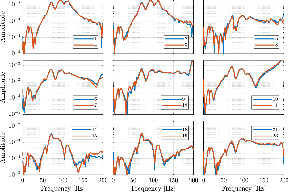
The response in the X direction of pairs of sensors aligned in the X direction are compared in Figure ref:fig:modal_solid_body_comp_x_dir. Good match is observed up to 200Hz. Similar result is obtained for the Y direction.

%% Load frequency response matrix
load('frf_matrix.mat', 'freqs', 'frf');

%% Accelerometers ID connected to each solid body
solids = {};
solids.gbot = [17, 18, 19, 20]; % bottom granite
solids.gtop = [13, 14, 15, 16]; % top granite
solids.ty   = [9, 10, 11, 12]; % Ty stage
solids.ry   = [5, 6, 7, 8]; % Ry stage
solids.rz   = [21, 22, 23]; % Rz stage
solids.hexa = [1, 2, 3, 4]; % Hexapod

% Names of the solid bodies
solid_names = fields(solids);

%% Save the acceleromter positions are well as the solid bodies
save('mat/geometry.mat', 'solids', 'solid_names', 'acc_pos');

%% Save the acceleromter positions are well as the solid bodies
save('matlab/mat/geometry.mat', 'solids', 'solid_names', 'acc_pos');

Comparaison of measured frequency response function for in the X directions for accelerometers aligned along X. Amplitude is in $\frac{m/s^2}{N}$. Accelerometer number is shown in the legend.

From accelerometer DOFs to solid body DOFs

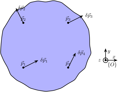
<<ssec:modal_acc_to_solid_dof>> Let's consider the schematic shown in Figure ref:fig:modal_local_to_global_coordinates where the motion of a solid body is measured at 4 distinct locations (in $x$, $y$ and $z$ directions).

The goal here is to link these $4 \times 3 = 12$ measurements to the 6 DOFs of the solid body expressed in the frame $\{O\}$.

  \newcommand\irregularcircle[2]{% radius, irregularity
    \pgfextra {\pgfmathsetmacro\len{(#1)+rand*(#2)}}
    +(0:\len pt)
    \foreach \a in {10,20,...,350}{
      \pgfextra {\pgfmathsetmacro\len{(#1)+rand*(#2)}}
      -- +(\a:\len pt)
    } -- cycle
  }
  \begin{tikzpicture}
    \draw[rounded corners=1mm, fill=blue!30!white] (0, 0) \irregularcircle{3cm}{1mm};

    \node[] (origin) at (4, -1) {$\bullet$};
    \begin{scope}[shift={(origin)}]
      \def\axissize{0.8cm}
      \draw[->] (0, 0) -- ++(\axissize, 0) node[above left]{$x$};
      \draw[->] (0, 0) -- ++(0, \axissize) node[below right]{$y$};
      \draw[fill, color=black] (0, 0) circle (0.05*\axissize);
      \node[draw, circle, inner sep=0pt, minimum size=0.4*\axissize, label=left:$z$] (yaxis) at (0, 0){};
      \node[below right] at (0, 0){$\{O\}$};
    \end{scope}

    \coordinate[] (p1) at (-1.5, -1.5);
    \coordinate[] (p2) at (-1.5,  1.5);
    \coordinate[] (p3) at ( 1.5,  1.5);
    \coordinate[] (p4) at ( 1.5, -1.5);

    \draw[->] (p1)node[]{$\bullet$}node[above]{$\vec{p}_1$} -- ++( 1  , 0.5)node[right]{$\delta \vec{p}_1$};
    \draw[->] (p2)node[]{$\bullet$}node[above]{$\vec{p}_2$} -- ++(-0.5, 1  )node[right]{$\delta \vec{p}_2$};
    \draw[->] (p3)node[]{$\bullet$}node[above]{$\vec{p}_3$} -- ++( 1  , 0.5)node[right]{$\delta \vec{p}_3$};
    \draw[->] (p4)node[]{$\bullet$}node[above]{$\vec{p}_4$} -- ++( 0.5, 1  )node[right]{$\delta \vec{p}_4$};
  \end{tikzpicture}

Schematic of the measured motions of a solid body

Let's consider the motion of the rigid body defined by its displacement $\delta \vec{p}$ and rotation $\delta\vec{\Omega}$ with respect to the reference frame $\{O\}$.

From the figure ref:fig:modal_local_to_global_coordinates, we can write:

\begin{align*} \delta \vec{p}_1 &= \delta \vec{p} + \bm{\delta \Omega} \vec{p}_1\\ \delta \vec{p}_2 &= \delta \vec{p} + \bm{\delta \Omega} \vec{p}_2\\ \delta \vec{p}_3 &= \delta \vec{p} + \bm{\delta \Omega} \vec{p}_3\\ \delta \vec{p}_4 &= \delta \vec{p} + \bm{\delta \Omega} \vec{p}_4 \end{align*}

With

\begin{equation} \bm{\delta\Omega} = \begin{bmatrix} 0 & -\delta\Omega_z & \delta\Omega_y \\ \delta\Omega_z & 0 & -\delta\Omega_x \\ -\delta\Omega_y & \delta\Omega_x & 0 \end{bmatrix} \end{equation}

We can rearrange the equations in a matrix form:

\begin{equation} \left[\begin{array}{ccc|ccc} 1 & 0 & 0 & 0 & p_{1z} & -p_{1y} \\ 0 & 1 & 0 & -p_{1z} & 0 & p_{1x} \\ 0 & 0 & 1 & p_{1y} & -p_{1x} & 0 \\ \hline & \vdots & & & \vdots & \\ \hline 1 & 0 & 0 & 0 & p_{4z} & -p_{4y} \\ 0 & 1 & 0 & -p_{4z} & 0 & p_{4x} \\ 0 & 0 & 1 & p_{4y} & -p_{4x} & 0 \end{array}\right] \left[\begin{array}{c} \delta p_x \\ \delta p_y \\ \delta p_z \\ \hline \delta\Omega_x \\ \delta\Omega_y \\ \delta\Omega_z \end{array}\right] = \left[\begin{array}{c} \delta p_{1x} \\ \delta p_{1y} \\ \delta p_{1z} \\\hline \vdots \\\hline \delta p_{4x} \\ \delta p_{4y} \\ \delta p_{4z} \end{array}\right] \end{equation}

and then we obtain the velocity and rotation of the solid in the wanted frame $\{O\}$:

\begin{equation} \left[\begin{array}{c} \delta p_x \\ \delta p_y \\ \delta p_z \\ \hline \delta\Omega_x \\ \delta\Omega_y \\ \delta\Omega_z \end{array}\right] = \left[\begin{array}{ccc|ccc} 1 & 0 & 0 & 0 & p_{1z} & -p_{1y} \\ 0 & 1 & 0 & -p_{1z} & 0 & p_{1x} \\ 0 & 0 & 1 & p_{1y} & -p_{1x} & 0 \\ \hline & \vdots & & & \vdots & \\ \hline 1 & 0 & 0 & 0 & p_{4z} & -p_{4y} \\ 0 & 1 & 0 & -p_{4z} & 0 & p_{4x} \\ 0 & 0 & 1 & p_{4y} & -p_{4x} & 0 \end{array}\right]^{-1} \left[\begin{array}{c} \delta p_{1x} \\ \delta p_{1y} \\ \delta p_{1z} \\\hline \vdots \\\hline \delta p_{4x} \\ \delta p_{4y} \\ \delta p_{4z} \end{array}\right] \label{eq:modal_determine_global_disp} \end{equation}

Using equation eqref:eq:modal_determine_global_disp, we can determine the motion of the solid body expressed in a chosen frame $\{O\}$ using the accelerometers attached to it. The inversion is equivalent to resolving a mean square problem.

Frequency Response Matrix expressed at the Center of Mass

<<ssec:modal_frf_com>>

What reference frame to choose?

The question we wish here to answer is how to choose the reference frame $\{O\}$ in which the DOFs of the solid bodies are defined.

The possibles choices are:

• One frame for each solid body which is located at its center of mass
• One common frame, for instance located at the point of interest ($270mm$ above the Hexapod)
• Base located at the joint position: this is where we want to see the motion and estimate stiffness

Chosen Frame	Advantages	Disadvantages
Frames at CoM	Physically, it makes more sense	How to compare the motion of the solid bodies?
Common Frame	We can compare the motion of each solid body	Small $\theta_{x, y}$ may result in large $T_{x, y}$
Frames at joint position	Directly gives which joint direction can be blocked	How to choose the joint position?

The choice of the frame depends of what we want to do with the data.

One of the goals is to compare the motion of each solid body to see which relative DOFs between solid bodies can be neglected, that is to say, which joint between solid bodies can be regarded as perfect (and this in all the frequency range of interest). Ideally, we would like to have the same number of degrees of freedom than the number of identified modes.

In the next sections, we will express the FRF matrix in the different frames.

Center of Mass of each solid body

From solidworks, we can export the position of the center of mass of each solid body considered. These are summarized in Table ref:tab:modal_com_solid_bodies

%% Extract the CoM of considered solid bodies
model_com = reshape(table2array(readtable('mat/model_solidworks_com.txt', 'ReadVariableNames', false)), [3, 6]);

	$X$ [mm]	$Y$ [mm]	$Z$ [mm]
Bottom Granite	45	144	-1251
Top granite	52	258	-778
Translation stage	0	14	-600
Tilt Stage	0	-5	-628
Spindle	0	0	-580
Hexapod	-4	6	-319

Computation

First, we initialize a new FRF matrix which is an $n \times p \times q$ with:

• $n$ is the number of DOFs of the considered 6 solid-bodies: $6 \times 6 = 36$
• $p$ is the number of excitation inputs: $3$
• $q$ is the number of frequency points $\omega_i$

For each frequency point $\omega_i$, the FRF matrix is a $n\times p$ matrix:

\begin{equation} \text{FRF}_\text{CoM}(\omega_i) = \begin{bmatrix} \frac{D_{1,T_x}}{F_x}(\omega_i) & \frac{D_{1,T_x}}{F_y}(\omega_i) & \frac{D_{1,T_x}}{F_z}(\omega_i) \\ \frac{D_{1,T_y}}{F_x}(\omega_i) & \frac{D_{1,T_y}}{F_y}(\omega_i) & \frac{D_{1,T_y}}{F_z}(\omega_i) \\ \frac{D_{1,T_z}}{F_x}(\omega_i) & \frac{D_{1,T_z}}{F_y}(\omega_i) & \frac{D_{1,T_z}}{F_z}(\omega_i) \\ \frac{D_{1,R_x}}{F_x}(\omega_i) & \frac{D_{1,R_x}}{F_y}(\omega_i) & \frac{D_{1,R_x}}{F_z}(\omega_i) \\ \frac{D_{1,R_y}}{F_x}(\omega_i) & \frac{D_{1,R_y}}{F_y}(\omega_i) & \frac{D_{1,R_y}}{F_z}(\omega_i) \\ \frac{D_{1,R_z}}{F_x}(\omega_i) & \frac{D_{1,R_z}}{F_y}(\omega_i) & \frac{D_{1,R_z}}{F_z}(\omega_i) \\ \frac{D_{2,T_x}}{F_x}(\omega_i) & \frac{D_{2,T_x}}{F_y}(\omega_i) & \frac{D_{2,T_x}}{F_z}(\omega_i) \\ \vdots & \vdots & \vdots \\ \frac{D_{6,R_z}}{F_x}(\omega_i) & \frac{D_{6,R_z}}{F_y}(\omega_i) & \frac{D_{6,R_z}}{F_z}(\omega_i) \end{bmatrix} \end{equation}

where 1, 2, …, 6 corresponds to the 6 solid bodies.

Then, as we know the positions of the accelerometers on each solid body, and we have the response of those accelerometers, we can use the equations derived in the previous section to determine the response of each solid body expressed in their center of mass.

%% Frequency Response Matrix - Response expressed at the CoM of the solid bodies
FRFs_CoM = zeros(length(solid_names)*6, 3, 801);

for solid_i = 1:length(solid_names)
  % Number of accelerometers fixed to this solid body
  solids_i = solids.(solid_names{solid_i});

  % "Jacobian" matrix to go from accelerometer frame to CoM frame
  A = zeros(3*length(solids_i), 6);
  for i = 1:length(solids_i)
    acc_i = solids_i(i);

    acc_pos_com = acc_pos(acc_i, :).' - model_com(:, solid_i);

    A(3*(i-1)+1:3*i, 1:3) = eye(3);
    A(3*(i-1)+1:3*i, 4:6) = [ 0               acc_pos_com(3) -acc_pos_com(2) ;
                             -acc_pos_com(3)  0               acc_pos_com(1) ;
                              acc_pos_com(2) -acc_pos_com(1)  0];
  end

  for exc_dir = 1:3
    FRFs_CoM((solid_i-1)*6+1:solid_i*6, exc_dir, :) = A\squeeze(frf((solids_i(1)-1)*3+1:solids_i(end)*3, exc_dir, :));
  end
end

%% Save the computed FRF at the CoM
save('mat/frf_com.mat', 'FRFs_CoM');

%% Save the computed FRF at the CoM
save('matlab/mat/frf_com.mat', 'FRFs_CoM');

Verify that we find the original FRF from the FRF in the global coordinates

<<ssec:modal_solid_body_assumption>>

We have computed the Frequency Response Functions Matrix representing the response of the 6 solid bodies in their 6 DOFs with respect to their center of mass.

From the response of one body in its 6 DOFs, we should be able to compute the FRF of each of its accelerometer fixed to it during the measurement, supposing that this stage is a solid body.

We can then compare the result with the original measurements. This will help us to determine if:

• the previous inversion used is correct
• the solid body assumption is correct in the frequency band of interest

From the translation $\delta p$ and rotation $\delta \Omega$ of a solid body and the positions $p_i$ of the accelerometers attached to it, we can compute the response that would have been measured by the accelerometers using the following formula:

\begin{align*} \delta p_1 &= \delta p + \delta\Omega p_1\\ \delta p_2 &= \delta p + \delta\Omega p_2\\ \delta p_3 &= \delta p + \delta\Omega p_3\\ \delta p_4 &= \delta p + \delta\Omega p_4 \end{align*}

Thus, we can obtain the FRF matrix FRFs_A that gives the responses of the accelerometers to the forces applied by the hammer.

It is implemented in matlab as follow:

FRFs_A = zeros(size(frf));

% For each excitation direction
for exc_dir = 1:3
  % For each solid
  for solid_i = 1:length(solid_names)
    v0 = squeeze(FRFs_CoM((solid_i-1)*6+1:(solid_i-1)*6+3, exc_dir, :));
    W0 = squeeze(FRFs_CoM((solid_i-1)*6+4:(solid_i-1)*6+6, exc_dir, :));

    % For each accelerometer attached to the current solid
    for acc_i = solids.(solid_names{solid_i})
      % We get the position of the accelerometer expressed in frame O
      pos = acc_pos(acc_i, :).' - model_com(:, solid_i);
      % pos = acc_pos(acc_i, :).';
      posX = [0 pos(3) -pos(2); -pos(3) 0 pos(1) ; pos(2) -pos(1) 0];

      FRFs_A(3*(acc_i-1)+1:3*(acc_i-1)+3, exc_dir, :) = v0 + posX*W0;
    end
  end
end

We then compare the original FRF measured for each accelerometer FRFs with the "recovered" FRF FRFs_A from the global FRF matrix in the common frame.

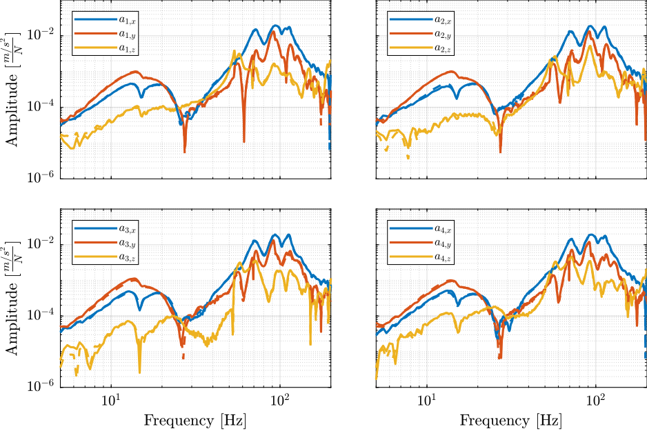
The FRF for the 4 accelerometers on the Hexapod are compared in Figure ref:fig:modal_comp_acc_solid_body_frf. All the FRF are matching very well in all the frequency range displayed.

Comparaison of the original accelerometer response and reconstructed response from the solid body response. For accelerometers 1 to 4 corresponding to the hexapod.

The reduction of the number of degrees of freedom from 69 (23 accelerometers with each 3DOF) to 36 (6 solid bodies with 6 DOF) seems to work well.

This confirms the fact that the stages are indeed behaving as a solid body in the frequency band of interest. This valid the fact that a multi-body model can be used to represent the dynamics of the micro-station.

Modal Analysis

<<sec:modal_analysis>>

Introduction   ignore

The goal here is to extract the modal parameters describing the modes of station being studied, namely:

• the eigen frequencies and the modal damping (eigen values)
• the mode shapes (eigen vectors)

This is done from the FRF matrix previously extracted from the measurements.

In order to do the modal parameter extraction, we first have to estimate the order of the modal model we want to obtain. This corresponds to how many modes are present in the frequency band of interest. In section ref:ssec:modal_number_of_modes, we will use the Singular Value Decomposition and the Modal Indication Function to estimate the number of modes.

The modal parameter extraction methods generally consists of curve-fitting a theoretical expression for an individual FRF to the actual measured data. However, there are multiple level of complexity:

• works on a part of a single FRF curve
• works on a complete curve encompassing several resonances
• works on a set of many FRF plots all obtained from the same structure

The third method is the most complex but gives better results. This is the one we will use in section ref:ssec:modal_parameter_extraction.

From the modal model, it is possible to obtain a graphic display of the mode shapes (section ref:ssec:modal_mode_shapes).

In order to validate the quality of the modal model, we will synthesize the FRF matrix from the modal model and compare it with the FRF measured (section ref:ssec:modal_model_validity).

The modes of the structure are expected to be complex, however real modes are easier to work with when it comes to obtain a spatial model from the modal parameters.

Determine the number of modes

<<ssec:modal_number_of_modes>>

Singular Value Decomposition - Modal Indication Function

The Mode Indicator Functions are usually used on $n\times p$ FRF matrix where $n$ is a relatively large number of measurement DOFs and $p$ is the number of excitation DOFs, typically 3 or 4.

In these methods, the frequency dependent FRF matrix is subjected to a singular value decomposition analysis which thus yields a small number (3 or 4) of singular values, these also being frequency dependent.

These methods are used to determine the number of modes present in a given frequency range, to identify repeated natural frequencies and to pre-process the FRF data prior to modal analysis.

From the documentation of the modal software:

The MIF consist of the singular values of the Frequency response function matrix. The number of MIFs equals the number of excitations. By the powerful singular value decomposition, the real signal space is separated from the noise space. Therefore, the MIFs exhibit the modes effectively. A peak in the MIFs plot usually indicate the existence of a structural mode, and two peaks at the same frequency point means the existence of two repeated modes. Moreover, the magnitude of the MIFs implies the strength of the a mode.

The Complex Mode Indicator Function is defined simply by the SVD of the FRF (sub) matrix:

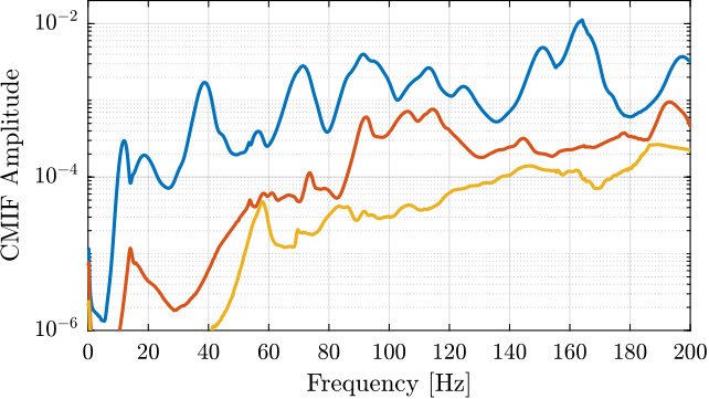
\begin{align*} [H(\omega)]_{n\times p} &= [U(\omega)]_{n\times n} [\Sigma(\omega)]_{n\times p} [V(\omega)]_{p\times p}^H\\ [CMIF(\omega)]_{p\times p} &= [\Sigma(\omega)]_{p\times n}^T [\Sigma(\omega)]_{n\times p} \end{align*}

We compute the Complex Mode Indicator Function. The result is shown on Figure ref:fig:modal_indication_function.

%% Computation of the modal indication function
MIF = zeros(size(frf, 2), size(frf, 2), size(frf, 3));

for i = 1:length(freqs)
  [~,S,~] = svd(frf(:, :, i));
  MIF(:, :, i) = S'*S;
end

Modal Indication Function

Composite Response Function

An alternative is the Composite Response Function $HH(\omega)$ defined as the sum of all the measured FRF:

\begin{equation} HH(\omega) = \sum_j\sum_kH_{jk}(\omega) \end{equation}

Instead, we choose here to use the sum of the norms of the measured frf:

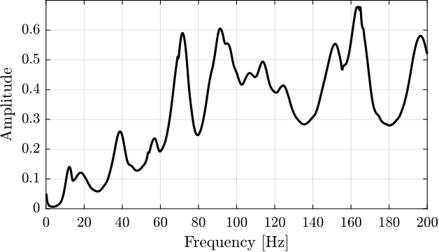
\begin{equation} HH(\omega) = \sum_j\sum_k \left|H_{jk}(\omega) \right| \end{equation}

The result is shown on figure ref:fig:modal_composite_reponse_function.

Composite Response Function

Modal parameter extraction

<<ssec:modal_parameter_extraction>>

OROS - Modal software

Modal identification are done within the Modal software of OROS.

Several modal parameter extraction methods are available. We choose to use the "broad band" method as it permits to identify the modal parameters using all the FRF curves at the same time. It takes into account the fact the the properties of all the individual curves are related by being from the same structure: all FRF plots on a given structure should indicate the same values for the natural frequencies and damping factor of each mode.

Such method also have the advantage of producing a unique and consistent model as direct output.

In order to apply this method, we select the frequency range of interest and we give an estimate of how many modes are present.

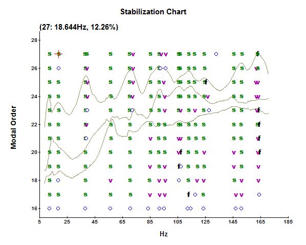
Then, it shows a stabilization charts, such as the one shown on figure ref:fig:modal_stabilization_chart, where we have to manually select which modes to take into account in the modal model.

We can then run the modal analysis, and the software will identify the modal damping and mode shapes at the selected frequency modes.

Importation of the modal parameters on Matlab

The obtained modal parameters are:

• Resonance frequencies in Hertz
• Modal damping ratio in percentage
• (complex) Modes shapes for each measured DoF
• Modal A and modal B which are parameters important for further normalization

%% Load modal parameters
shapes_m = readtable('mat/mode_shapes.txt',              'ReadVariableNames', false);  % [Sign / Real / Imag]
freqs_m  = table2array(readtable('mat/mode_freqs.txt',   'ReadVariableNames', false)); % in [Hz]
damps_m  = table2array(readtable('mat/mode_damps.txt',   'ReadVariableNames', false)); % in [%]
modal_a  = table2array(readtable('mat/mode_modal_a.txt', 'ReadVariableNames', false)); % [Real / Imag]
modal_b  = table2array(readtable('mat/mode_modal_b.txt', 'ReadVariableNames', false)); % [Real / Imag]

%% Guess the number of modes identified from the length of the imported data.
acc_n = 23; % Number of accelerometers
dir_n = 3; % Number of directions
dirs = 'XYZ';

mod_n = size(shapes_m,1)/acc_n/dir_n; % Number of modes

%% Mode shapes are split into 3 parts (direction plus sign, real part and imaginary part)
% we aggregate them into one array of complex numbers
T_sign = table2array(shapes_m(:, 1));
T_real = table2array(shapes_m(:, 2));
T_imag = table2array(shapes_m(:, 3));

mode_shapes = zeros(mod_n, dir_n, acc_n);

for mod_i = 1:mod_n
  for acc_i = 1:acc_n
    % Get the correct section of the signs
    T = T_sign(acc_n*dir_n*(mod_i-1)+1:acc_n*dir_n*mod_i);
    for dir_i = 1:dir_n
      % Get the line corresponding to the sensor
      i = find(contains(T, sprintf('%i%s',acc_i, dirs(dir_i))), 1, 'first')+acc_n*dir_n*(mod_i-1);
      mode_shapes(mod_i, dir_i, acc_i) = str2num([T_sign{i}(end-1), '1'])*complex(T_real(i),T_imag(i));
    end
  end
end

The obtained mode frequencies and damping are shown in Table ref:tab:modal_obtained_modes_freqs_damps.

Mode	Frequency [Hz]	Damping [%]
1	11.9	12.2
2	18.6	11.7
3	37.8	6.2
4	39.1	2.8
5	56.3	2.8
6	69.8	4.3
7	72.5	1.3
8	84.8	3.7
9	91.3	2.9
10	105.5	3.2
11	106.6	1.6
12	112.7	3.1
13	124.2	2.8
14	145.3	1.3
15	150.5	2.4
16	165.4	1.4

Theory

It seems that the modal analysis software makes the assumption of viscous damping for the model with which it tries to fit the FRF measurements.

If we note $N$ the number of modes identified, then there are $2N$ eigenvalues and eigenvectors given by the software:

\begin{align} s_r &= \omega_r (-\xi_r + i \sqrt{1 - \xi_r^2}),\quad s_r^* \\ \{\psi_r\} &= \begin{Bmatrix} \psi_{1_x} & \psi_{2_x} & \dots & \psi_{23_x} & \psi_{1_y} & \dots & \psi_{1_z} & \dots & \psi_{23_z} \end{Bmatrix}^T, \quad \{\psi_r\}^* \end{align}

for $r = 1, \dots, N$ where $\omega_r$ is the natural frequency and $\xi_r$ is the critical damping ratio for that mode.

Modal Matrices

We would like to arrange the obtained modal parameters into two modal matrices: \[ \Lambda = \begin{bmatrix} s_1 & & 0 \\ & \ddots & \\ 0 & & s_N \end{bmatrix}_{N \times N}; \quad \Psi = \begin{bmatrix} & & \\ \{\psi_1\} & \dots & \{\psi_N\} \\ & & \end{bmatrix}_{M \times N} \] \[ \{\psi_i\} = \begin{Bmatrix} \psi_{i, 1_x} & \psi_{i, 1_y} & \psi_{i, 1_z} & \psi_{i, 2_x} & \dots & \psi_{i, 23_z} \end{Bmatrix}^T \]

$M$ is the number of DoF: here it is $23 \times 3 = 69$. $N$ is the number of mode

eigen_val_M = diag(2*pi*freqs_m.*(-damps_m/100 + j*sqrt(1 - (damps_m/100).^2)));
eigen_vec_M = reshape(mode_shapes, [mod_n, acc_n*dir_n]).';

Each eigen vector is normalized: $\| \{\psi_i\} \|_2 = 1$

However, the eigen values and eigen vectors appears as complex conjugates: \[ s_r, s_r^*, \{\psi\}_r, \{\psi\}_r^*, \quad r = 1, N \]

In the end, they are $2N$ eigen values. We then build two extended eigen matrices as follow: \[ \mathcal{S} = \begin{bmatrix} s_1 & & & & & \\ & \ddots & & & 0 & \\ & & s_N & & & \\ & & & s_1^* & & \\ & 0 & & & \ddots & \\ & & & & & s_N^* \end{bmatrix}_{2N \times 2N}; \quad \Phi = \begin{bmatrix} & & & & &\\ \{\psi_1\} & \dots & \{\psi_N\} & \{\psi_1^*\} & \dots & \{\psi_N^*\} \\ & & & & & \end{bmatrix}_{M \times 2N} \]

eigen_val_ext_M = blkdiag(eigen_val_M, conj(eigen_val_M));
eigen_vec_ext_M = [eigen_vec_M, conj(eigen_vec_M)];

We also build the Modal A and Modal B matrices:

\begin{equation} A = \begin{bmatrix} a_1 & & 0 \\ & \ddots & \\ 0 & & a_N \end{bmatrix}_{N \times N}; \quad B = \begin{bmatrix} b_1 & & 0 \\ & \ddots & \\ 0 & & b_N \end{bmatrix}_{N \times N} \end{equation}

With $a_i$ is the "Modal A" parameter linked to mode i.

modal_a_M = diag(complex(modal_a(:, 1), modal_a(:, 2)));
modal_b_M = diag(complex(modal_b(:, 1), modal_b(:, 2)));

modal_a_ext_M = blkdiag(modal_a_M, conj(modal_a_M));
modal_b_ext_M = blkdiag(modal_b_M, conj(modal_b_M));

"Modal A" and "modal B" are linked through the following formula: \[ B = - A \Lambda \]

Obtained Mode Shapes animations

<<ssec:modal_mode_shapes>> From the modal parameters, it is possible to show the modal shapes with an animation.

Examples are shown in Figures ref:fig:modal_mode_animations.

Instrumentation used for the modal analysis

We can learn quite a lot from these mode shape animations.

For instance, the mode shape of the first mode at 11Hz (figure ref:fig:modal_mode1_animation) seems to indicate that this corresponds to a suspension mode.

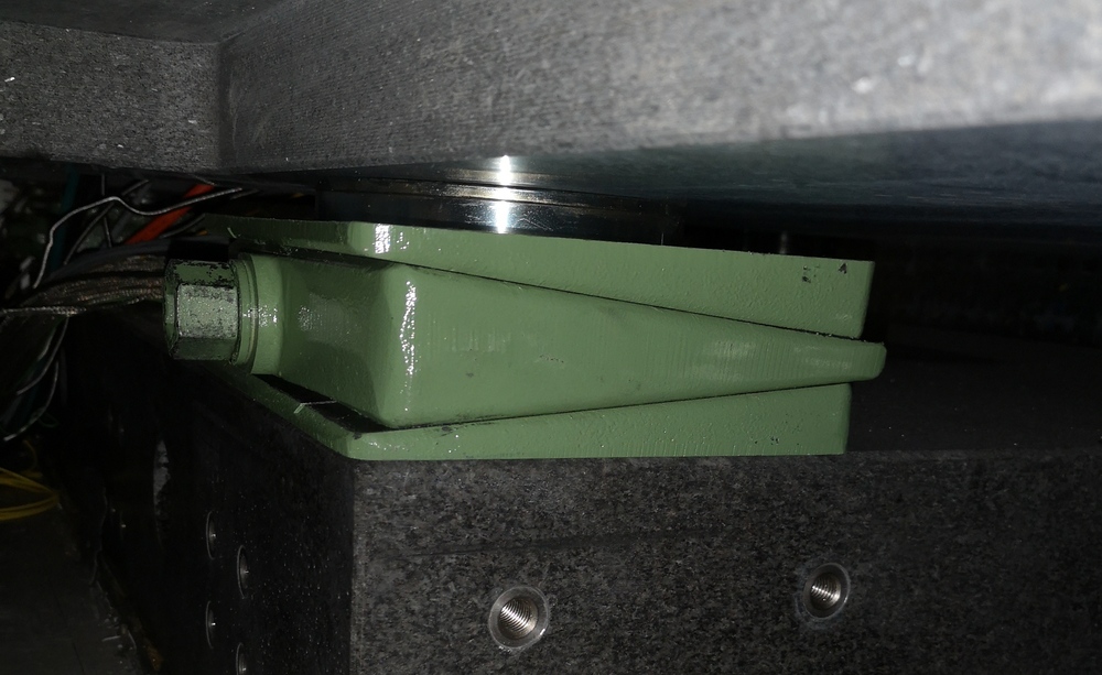
This could be due to the 4 Airloc Levelers that are used for the granite (figure ref:fig:modal_airloc).

They are probably not well leveled, so the granite is supported only by two Airloc.

Verify the validity of the Modal Model

<<ssec:modal_model_validity>>

There are two main ways to verify the validity of the modal model

• Synthesize FRF measurements that has been used to generate the modal model and compare
• Synthesize FRF that has not yet been measured. Then measure that FRF and compare

From the modal model, we want to synthesize the Frequency Response Functions that has been used to build the modal model.

Let's recall that:

• $M$ is the number of measured DOFs ($3 \times n_\text{acc}$)
• $N$ is the number of modes identified

We then have that the FRF matrix $[H_{\text{syn}}]$ can be synthesize using the following formula:

\begin{equation} [H_{\text{syn}}(\omega)]_{M\times M} = [\Phi]_{M\times2N} \left[\frac{Q_r}{j\omega - s_r}\right]_{2N\times2N} [\Phi]_{2N\times M}^T \end{equation}

with $Q_r = 1/M_{A_r}$

An alternative formulation is: \[ H_{pq}(s_i) = \sum_{r=1}^N \frac{A_{pqr}}{s_i - \lambda_r} + \frac{A_{pqr}^*}{s_i - \lambda_r^*} \] with:

• $A_{pqr} = \frac{\psi_{pr}\psi_{qr}}{M_{A_r}}$, $M_{A_r}$ is called "Modal A"
• $\psi_{pr}$: scaled modal coefficient for output DOF $p$, mode $r$
• $\lambda_r$: complex modal frequency

From the modal software documentation:

Modal A Scaling constant for a complex mode. It has the same properties as modal mass for normal modes (undamped or proportionally damped cases). Assuming

• $\psi_{pr}$ = Modal coefficient for measured degree of freedom p and mode r
• $\psi_{qr}$ = Modal coefficient for measured degree of freedom q and mode r
• $A_{pqr}$ = Residue for measured degree of freedom p, measured degree of q and mode r
• $M_{Ar}$ = Modal A of mode r

Then \[ A_{pqr} = \frac{\psi_{pr}\psi_{qr}}{M_{Ar}} \]

Modal B Scaling constant for a complex mode. It has the same properties as modal stiffness for normal modes (undamped or proportionally damped cases). Assuming

• $M_{Ar}$ = Modal A of mode r
• $\lambda_r$ = System pole of mode r

Then \[ M_{Br} = - \lambda_r M_{Ar} \]

%% Synthesize FRF from the modal model
Hsyn = zeros(acc_n*dir_n, acc_n*dir_n, length(freqs));

for i = 1:length(freqs)
  Hsyn(:, :, i) = eigen_vec_ext_M*((j*2*pi*freqs(i)).^2*inv(modal_a_ext_M)/(diag(j*2*pi*freqs(i) - diag(eigen_val_ext_M))))*eigen_vec_ext_M.';
end

%% Derivate two times to to have the acceleration response
for i = 1:size(Hsyn, 1)
  Hsyn(i, :, :) = squeeze(Hsyn(i, :, :)).*(j*2*pi*freqs).^2;
end

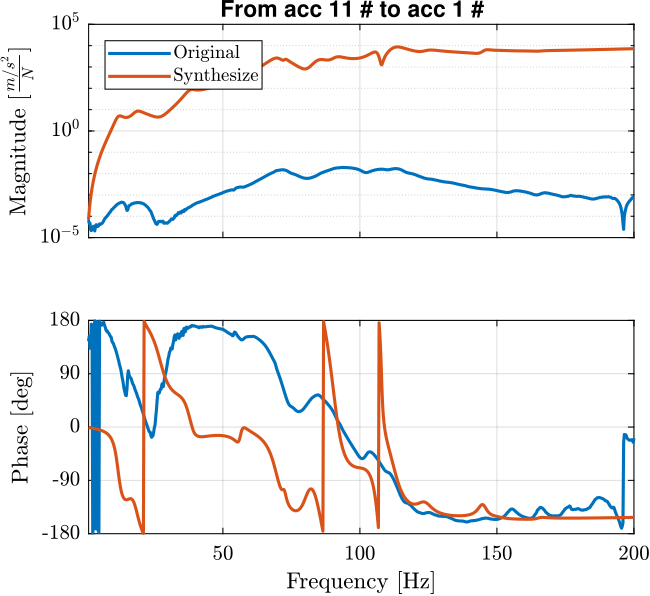
The comparison between the original measured frequency response function and the synthesized one from the modal model is done in Figure ref:fig:modal_comp_acc_frf_modal.

description

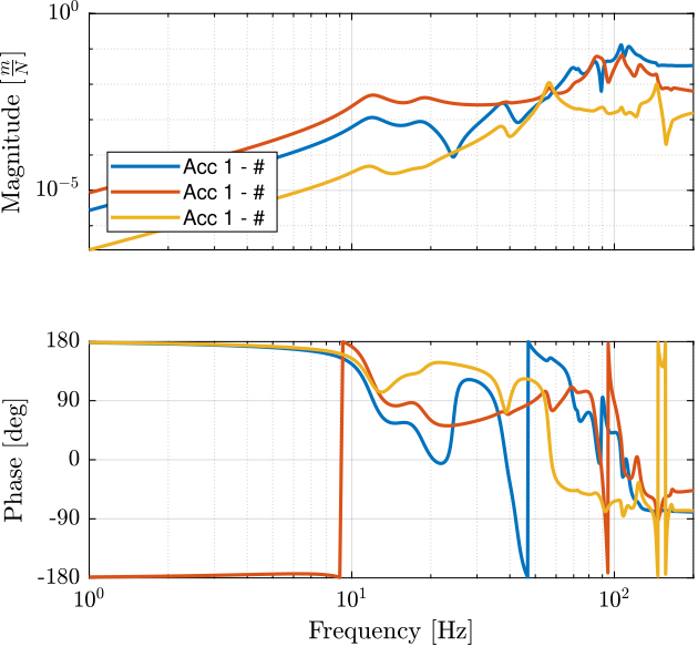
Frequency response functions that has not been measured can be synthesized as shown in Figure ref:fig:modal_synthesized_frf.

description

Conclusion

<<sec:modal_conclusion>>

Validation of solid body model.

Further step: go from modal model to parameters of the solid body model.

Bibliography   ignore