phd-control/nass-control.org

Control Optimization

• Introduction
• Multiple Sensor Control
  • Introduction
  • Review of Sensor Fusion
  • Sensor Fusion and Complementary Filters Requirements
    • Sensor Fusion Architecture
    • Sensor Models and Sensor Normalization
    • Noise Sensor Filtering
    • Sensor Fusion Robustness
  • Complementary Filters Shaping
    • Introduction
    • Synthesis Objective
    • Shaping of Complementary Filters using $\mathcal{H}_\infty$ synthesis
    • Weighting Functions Design
    • Validation of the proposed synthesis method
  • Synthesis of a set of three complementary filters
  • Conclusion
• Decoupling
  • Introduction
  • Test Model
  • Control in the frame of the struts
  • Jacobian Decoupling
    • Jacobian Matrix
    • Center Of Mass
    • Center Of Stiffness
  • Modal Decoupling
    • Theory
    • Example
  • SVD Decoupling
    • Singular Value Decomposition
    • Decoupling using the SVD
    • Example
  • Comparison of decoupling strategies
• Closed-Loop Shaping using Complementary Filters
  • Introduction
  • Control Architecture
    • Virtual Sensor Fusion
    • Asymptotic behavior
  • Translating the performance requirements into the shapes of the complementary filters
    • Introduction
    • Nominal Stability (NS)
    • Nominal Performance (NP)
    • Response time to change of reference signal
    • Input usage
    • Robust Stability (RS)
    • Robust Performance (RP)
  • Complementary filter design
  • Numerical Example
    • Procedure
    • Plant
    • Requirements and choice of complementary filters
    • Controller analysis
    • Robustness and Performance analysis
  • Conclusion
• Conclusion
• Bibliography
• Footnotes

Introduction   ignore

When controlling a MIMO system (specifically parallel manipulator such as the Stewart platform?)

• Should the quick review of Stewart platform control be here? In that case it should be possible to highlight three areas:

  • use of multiple sensors
  • decoupling strategy
  • control optimization

Several considerations:

• Section ref:sec:detail_control_sensor: How to most effectively use/combine multiple sensors
• Section ref:sec:detail_control_decoupling: How to decouple a system
• Section ref:sec:detail_control_cf: How to design the controller

Multiple Sensor Control

<<sec:detail_control_sensor>>

Introduction   ignore

The literature review of Stewart platforms revealed a wide diversity of designs with various sensor and actuator configurations. Control objectives (such as active damping, vibration isolation, or precise positioning) dictate specific sensor configurations. The selection between inertial sensors, force sensors, or relative position sensors is primarily determined by the system's control requirements.

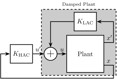
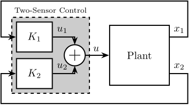
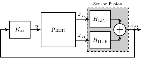
In cases where multiple control objectives must be achieved simultaneously, as is the case for the Nano Active Stabilization System (NASS) where the Stewart platform must both position the sample and provide isolation from micro-station vibrations, combining multiple sensors within the control architecture has been demonstrated to yield significant performance benefits. From the literature, three principal approaches for combining sensors have been identified: High Authority Control-Low Authority Control (HAC-LAC), sensor fusion, and two-sensor control architectures.

\begin{tikzpicture}
  % Blocs
  \node[block={2.0cm}{2.0cm}] (P) {Plant};
  \coordinate[] (input)   at ($(P.south west)!0.5!(P.north west)$);
  \coordinate[] (outputH) at ($(P.south east)!0.2!(P.north east)$);
  \coordinate[] (outputL) at ($(P.south east)!0.8!(P.north east)$);

  \node[block, above=0.2 of P] (Klac) {$K_\text{LAC}$};
  \node[addb, left=0.5 of input] (addF) {};
  \node[block, left=0.6 of addF] (Khac) {$K_\text{HAC}$};
  % \node[addb={+}{}{}{}{-}, left=0.5 of Khac] (subr) {};

  % Connections and labels
  \draw[->] (outputL) -- ++(0.5, 0) coordinate(eastlac) |- (Klac.east);
  \node[above right] at (outputL){$x^\prime$};
  \draw[->] (Klac.west) -| (addF.north);
  \draw[->] (addF.east) -- (input) node[above left]{$u$};

  % \draw[<-] (subr.west)node[above left]{$r$} -- ++(-0.5, 0);
  % \draw[->] (outputH) -- ++(0.5, 0)  -- ++(0, -1.0) -| (subr.south);
  \draw[->] (outputH) -- ++(0.5, 0)  -- ++(0, -0.7) -| ($(Khac.west)+(-0.5, 0)$) -- (Khac.west);
  \node[above right] at (outputH){$x$};
  % \draw[->] (subr.east) -- (Khac.west) node[above left]{$\epsilon$};
  \draw[->] (Khac.east) node[above right]{$u^\prime$} -- (addF.west);

  \begin{scope}[on background layer]
    \node[fit={(Klac.north-|eastlac) (addF.west|-P.south)}, fill=black!20!white, draw, dashed, inner sep=4pt] (Pi) {};
    % \node[anchor={north west}, align=left] at (Pi.north west){\scriptsize{Damped}\\\scriptsize{Plant}};
    \node[above=0 of Pi]{\scriptsize{Damped Plant}};
  \end{scope}
\end{tikzpicture}

\begin{tikzpicture}
  % Blocs
  \node[block={2.0cm}{2.0cm}] (P) {Plant};
  \coordinate[] (input)    at ($(P.south west)!0.5!(P.north west)$);
  \coordinate[] (outputH)  at ($(P.south east)!0.2!(P.north east)$);
  \coordinate[] (outputL)  at ($(P.south east)!0.8!(P.north east)$);
  \coordinate[] (outputSS) at ($(P.south east)!0.5!(P.north east)$);

  \node[block, right=0.8 of outputH] (KH) {$H_\text{HPF}$};
  \node[block, right=0.8 of outputL] (KL) {$H_\text{LPF}$};
  \node[addb={+}{}{}{}{}, right=2.2 of outputSS] (addss) {};
  \node[block, left=0.6 of input] (K) {$K_{ss}$};

  % Connections and labels
  \draw[->] (outputL) -- (KL.west);
  \draw[->] (outputH) -- (KH.west);
  \node[above right] at (outputL){$x_L$};
  \node[above right] at (outputH){$x_H$};
  \draw[->] (KL.east) -| (addss.north);
  \draw[->] (KH.east) -| (addss.south);
  \draw[->] (addss.east) -- ++(0.9, 0);
  \draw[->] ($(addss.east) + (0.5, 0)$)node[branch]{}node[above]{$x_{ss}$} -- ++(0, -1.6) -| ($(K.west)+(-0.5, 0)$) -- (K.west);
  \draw[->] (K.east) -- (input) node[above left]{$u$};

  \begin{scope}[on background layer]
    \node[fit={(KL.north west) (KH.south-|addss.east)}, fill=black!20!white, draw, dashed, inner sep=4pt] (Pss) {};
    \node[above=0 of Pss]{\scriptsize{Sensor Fusion}};
  \end{scope}
\end{tikzpicture}

\begin{tikzpicture}
  % Blocs
  \node[block={2.0cm}{2.0cm}] (P) {Plant};
  \coordinate[] (input)    at ($(P.south west)!0.5!(P.north west)$);
  \coordinate[] (output1)  at ($(P.south east)!0.8!(P.north east)$);
  \coordinate[] (output2)  at ($(P.south east)!0.2!(P.north east)$);

  \node[addb={+}{}{}{}{}, left=0.8 of input] (addF) {};
  \coordinate[left= 1.0 of addF] (Ks);
  \node[block] (K1) at (Ks|-output1) {$K_\text{1}$};
  \node[block] (K2) at (Ks|-output2) {$K_\text{2}$};

  \draw[->] (output1) -| ++(0.6, 1.2) -| ($(K1.west)+(-0.5, 0)$) -- (K1.west);
  \draw[->] (output2) -| ++(0.6,-1.0) -| ($(K2.west)+(-0.5, 0)$) -- (K2.west);

  \draw[->] (K1.east)node[above right]{$u_1$} -| (addF.north);
  \draw[->] (K2.east)node[above right]{$u_2$} -| (addF.south);
  \draw[->] (addF.east) -- (input) node[above left=0 and 0.2]{$u$};

  \node[above right] at (output1){$x_1$};
  \node[above right] at (output2){$x_2$};

  \begin{scope}[on background layer]
    \node[fit={(K1.north west) (K2.south-|addF.east)}, fill=black!20!white, draw, dashed, inner sep=4pt] (Pss) {};
    \node[above=0 of Pss]{\scriptsize{Two-Sensor Control}};
  \end{scope}
\end{tikzpicture}

\bigskip

The HAC-LAC approach, implemented during the conceptual phase, employs a dual-loop control strategy in which two control loops utilize different sensors for distinct purposes (Figure ref:fig:detail_control_sensor_arch_hac_lac). In cite:&li01_simul_vibrat_isolat_point_contr, vibration isolation is provided by accelerometers collocated with the voice coil actuators, while external rotational sensors are utilized to achieve pointing control. In cite:&geng95_intel_contr_system_multip_degree, force sensors collocated with the magnetostrictive actuators are used for active damping using decentralized IFF, and subsequently accelerometers are employed for adaptive vibration isolation. Similarly, in cite:&wang16_inves_activ_vibrat_isolat_stewar, piezoelectric actuators with collocated force sensors are used in a decentralized manner to provide active damping while accelerometers are implemented in an adaptive feedback loop to suppress periodic vibrations. In cite:&xie17_model_contr_hybrid_passiv_activ, force sensors are integrated in the struts for decentralized force feedback while accelerometers fixed to the top platform are employed for centralized control.

The second approach, sensor fusion (illustrated in Figure ref:fig:detail_control_sensor_arch_sensor_fusion), involves filtering signals from two sensors using complementary filters¹ and summing them to create an improved sensor signal. In cite:&hauge04_sensor_contr_space_based_six, geophones (used at low frequency) are merged with force sensors (used at high frequency). It is demonstrated that combining both sensors using sensor fusion can improve performance compared to using the individual sensors independently. In cite:&tjepkema12_sensor_fusion_activ_vibrat_isolat_precis_equip, sensor fusion architecture is implemented with an accelerometer and a force sensor. This implementation is shown to simultaneously achieve high damping of structural modes (through the force sensors) while maintaining very low vibration transmissibility (through the accelerometers).

In cite:&beijen14_two_sensor_contr_activ_vibrat, the performance of sensor fusion is compared with the more general case of "two-sensor control" (illustrated in Figure ref:fig:detail_control_sensor_arch_two_sensor_control). It is highlighted that "two-sensor control" provides greater control freedom, potentially enhancing performance. In cite:&thayer02_six_axis_vibrat_isolat_system, the use of force sensors and geophones is compared for vibration isolation purposes. Geophones are shown to provide better isolation performance than load cells but suffer from poor robustness. Conversely, the controller based on force sensors exhibited inferior performance (due to the presence of a pair of low frequency zeros), but demonstrated better robustness properties. A "two-sensor control" approach was proven to perform better than controllers based on individual sensors while maintaining better robustness. A Linear Quadratic Regulator (LQG) was employed to optimize the two-input/one-output controller.

Beyond these three main approaches, other control architectures have been proposed for different purposes. In cite:&yang19_dynam_model_decoup_contr_flexib, a first control loop utilizes force sensors and relative motion sensors to compensate for parasitic stiffness of the flexible joints. Subsequently, the system is decoupled in the modal space (facilitated by the removal of parasitic stiffness) and accelerometers are employed for vibration isolation.

The HAC-LAC architecture was previously investigated during the conceptual phase and successfully implemented to validate the NASS concept, demonstrating excellent performance. At the other end of the spectrum, the two-sensor approach yields greater control design freedom but introduces increased complexity in tuning, and thus was not pursued in this study. This work instead focuses on sensor fusion, which represents a promising middle ground between the proven HAC-LAC approach and the more complex two-sensor control strategy.

A review of sensor fusion is first presented (Section ref:ssec:detail_control_sensor_review), followed by an examination of the fundamental theoretical concepts (Section ref:ssec:detail_control_sensor_fusion_requirements). In this section, both the robustness of the fusion and the noise characteristics of the resulting "super sensor" are derived and expressed as functions of the complementary filters' norms. A synthesis method for designing complementary filters that allow to shape their norms is proposed (Section ref:ssec:detail_control_sensor_hinf_method). The investigation is then extended beyond the conventional two-sensor scenario, demonstrating how the proposed complementary filter synthesis can be generalized for applications requiring the fusion of three or more sensors (Section ref:ssec:detail_control_sensor_hinf_three_comp_filters).

Review of Sensor Fusion

<<ssec:detail_control_sensor_review>>

Sensors used to measure physical quantities have two primary limitations: measurement accuracy which is compromised by various noise sources (including electrical noise from conditioning electronics), and limited measurement bandwidth. Sensor fusion offers a solution to these limitations by combining multiple sensors cite:&bendat57_optim_filter_indep_measur_two. By strategically selecting sensors with complementary characteristics, a "super sensor" can be created that combines the advantages of each individual sensor.

Measuring a physical quantity using sensors is always subject to several limitations. First, the accuracy of the measurement is affected by various noise sources, such as electrical noise from the conditioning electronics. Second, the frequency range in which the measurement is relevant is bounded by the bandwidth of the sensor. One way to overcome these limitations is to combine several sensors using a technique called "sensor fusion" cite:&bendat57_optim_filter_indep_measur_two. Fortunately, a wide variety of sensors exists, each with different characteristics. By carefully selecting the sensors to be fused, a "super sensor" is obtained that combines the benefits of the individual sensors.

In some applications, sensor fusion is employed to increase measurement bandwidth cite:&shaw90_bandw_enhan_posit_measur_using_measur_accel;&zimmermann92_high_bandw_orien_measur_contr;&min15_compl_filter_desig_angle_estim. For instance, in cite:&shaw90_bandw_enhan_posit_measur_using_measur_accel, the bandwidth of a position sensor is extended by fusing it with an accelerometer that provides high-frequency motion information. In other applications, sensor fusion is utilized to obtain an estimate of the measured quantity with reduced noise cite:&hua05_low_ligo;&hua04_polyp_fir_compl_filter_contr_system;&plummer06_optim_compl_filter_their_applic_motion_measur;&robert12_introd_random_signal_applied_kalman. More recently, the fusion of sensors measuring different physical quantities has been proposed to enhance control properties cite:&collette15_sensor_fusion_method_high_perfor;&yong16_high_speed_vertic_posit_stage. In cite:&collette15_sensor_fusion_method_high_perfor, an inertial sensor used for active vibration isolation is fused with a sensor collocated with the actuator to improve the stability margins of the feedback controller.

On top of Stewart platforms, practical applications of sensor fusion are numerous. It is widely implemented for attitude estimation in autonomous vehicles such as unmanned aerial vehicles cite:&baerveldt97_low_cost_low_weigh_attit;&corke04_inert_visual_sensin_system_small_auton_helic;&jensen13_basic_uas and underwater vehicles cite:&pascoal99_navig_system_desig_using_time;&batista10_optim_posit_veloc_navig_filter_auton_vehic. Sensor fusion offers significant benefits for high-performance positioning control as demonstrated in cite:&shaw90_bandw_enhan_posit_measur_using_measur_accel;&zimmermann92_high_bandw_orien_measur_contr;&min15_compl_filter_desig_angle_estim;&yong16_high_speed_vertic_posit_stage. It has also been identified as a key technology for improving the performance of active vibration isolation systems cite:&tjepkema12_sensor_fusion_activ_vibrat_isolat_precis_equip. Emblematic examples include the isolation stages of gravitational wave detectors cite:&collette15_sensor_fusion_method_high_perfor;&heijningen18_low such as those employed at LIGO cite:&hua05_low_ligo;&hua04_polyp_fir_compl_filter_contr_system and Virgo cite:&lucia18_low_frequen_optim_perfor_advan.

Two principal methods are employed to perform sensor fusion: using complementary filters cite:&anderson53_instr_approac_system_steer_comput or using Kalman filtering cite:&brown72_integ_navig_system_kalman_filter. For sensor fusion applications, these methods share many relationships cite:&brown72_integ_navig_system_kalman_filter;&higgins75_compar_compl_kalman_filter;&robert12_introd_random_signal_applied_kalman;&fonseca15_compl. However, Kalman filtering requires assumptions about the probabilistic characteristics of sensor noise cite:&robert12_introd_random_signal_applied_kalman, whereas complementary filters do not impose such requirements. Furthermore, complementary filters offer advantages over Kalman filtering for sensor fusion through their general applicability, low computational cost cite:&higgins75_compar_compl_kalman_filter, and intuitive nature, as their effects can be readily interpreted in the frequency domain.

A set of filters is considered complementary if the sum of their transfer functions equals one at all frequencies. In early implementations of complementary filtering, analog circuits were used to physically realize the filters cite:&anderson53_instr_approac_system_steer_comput. While analog complementary filters remain in use today cite:&yong16_high_speed_vertic_posit_stage;&moore19_capac_instr_sensor_fusion_high_bandw_nanop, digital implementation is now more common as it provides greater flexibility.

Various design methods have been developed to optimize complementary filters. The most straightforward approach utilizes analytical formulas. Depending on the application, these formulas may be of first order cite:&corke04_inert_visual_sensin_system_small_auton_helic;&yeh05_model_contr_hydraul_actuat_two;&yong16_high_speed_vertic_posit_stage, second order cite:&baerveldt97_low_cost_low_weigh_attit;&stoten01_fusion_kinet_data_using_compos_filter;&jensen13_basic_uas, or higher orders cite:&shaw90_bandw_enhan_posit_measur_using_measur_accel;&zimmermann92_high_bandw_orien_measur_contr;&stoten01_fusion_kinet_data_using_compos_filter;&collette15_sensor_fusion_method_high_perfor;&matichard15_seism_isolat_advan_ligo.

Since the characteristics of the super sensor depend on the proper design of complementary filters cite:&dehaeze19_compl_filter_shapin_using_synth, several optimization techniques have been developed. Some approaches focus on finding optimal parameters for analytical formulas cite:&jensen13_basic_uas;&min15_compl_filter_desig_angle_estim;&fonseca15_compl, while others employ convex optimization tools cite:&hua04_polyp_fir_compl_filter_contr_system;&hua05_low_ligo such as linear matrix inequalities cite:&pascoal99_navig_system_desig_using_time. As demonstrated in cite:&plummer06_optim_compl_filter_their_applic_motion_measur, complementary filter design can be linked to the standard mixed-sensitivity control problem. Consequently, the powerful tools developed for classical control theory can be applied to complementary filter design. For example, in cite:&jensen13_basic_uas, the two gains of a Proportional Integral (PI) controller are optimized to minimize super sensor noise.

All these complementary filter design methods share the common objective of creating a super sensor with desired characteristics, typically in terms of noise and dynamics. As reported in cite:&zimmermann92_high_bandw_orien_measur_contr;&plummer06_optim_compl_filter_their_applic_motion_measur, phase shifts and magnitude bumps in the super sensor dynamics may occur if complementary filters are poorly designed or if sensors are improperly calibrated. Therefore, the robustness of the fusion must be considered when designing complementary filters. Despite the numerous design methods proposed in the literature, a simple approach that specifies desired super sensor characteristics while ensuring good fusion robustness has been lacking.

Fortunately, both fusion robustness and super sensor characteristics can be linked to complementary filter magnitude cite:&dehaeze19_compl_filter_shapin_using_synth. Based on this relationship, the present work introduces an approach to designing complementary filters using $\mathcal{H}_\infty$ synthesis, which enables intuitive shaping of complementary filter magnitude in a straightforward manner.

Sensor Fusion and Complementary Filters Requirements

<<ssec:detail_control_sensor_fusion_requirements>>

Sensor Fusion Architecture   ignore

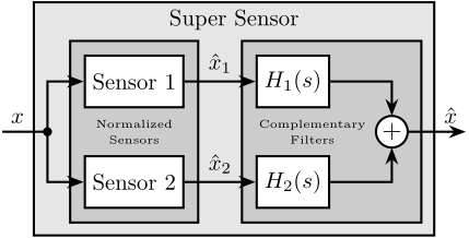
A general sensor fusion architecture using complementary filters is shown in Figure ref:fig:detail_control_sensor_fusion_overview, where multiple sensors (in this case two) measure the same physical quantity $x$. The sensor output signals $\hat{x}_1$ and $\hat{x}_2$ represent estimates of $x$. These estimates are filtered by complementary filters and combined to form a new estimate $\hat{x}$.

\tikzset{block/.default={0.8cm}{0.8cm}}
\tikzset{addb/.append style={scale=0.7}}
\tikzset{node distance=0.6}
\begin{tikzpicture}
  \node[branch] (x) at (0, 0);
  \node[block, above right=0.3 and 0.5 of x](sensor1){Sensor 1};
  \node[block, below right=0.3 and 0.5 of x](sensor2){Sensor 2};

  \node[block, right=1.1 of sensor1](H1){$H_1(s)$};
  \node[block, right=1.1 of sensor2](H2){$H_2(s)$};

  \node[addb, right=5.0 of x](add){};

  \draw[] ($(x)+(-0.7, 0)$) node[above right]{$x$} -- (x.center);
  \draw[->] (x.center) |- (sensor1.west);
  \draw[->] (x.center) |- (sensor2.west);
  \draw[->] (sensor1.east) -- node[midway, above]{$\hat{x}_1$} (H1.west);
  \draw[->] (sensor2.east) -- node[midway, above]{$\hat{x}_2$} (H2.west);
  \draw[->] (H1) -| (add.north);
  \draw[->] (H2) -| (add.south);
  \draw[->] (add.east) -- ++(0.9, 0) node[above left]{$\hat{x}$};

  \begin{scope}[on background layer]
    \node[fit={($(H2.south-|x) + (0, -0.2)$) ($(H1.north-|add.east) + (0.2, 0.6)$)}, fill=black!10!white, draw, inner sep=6pt] (supersensor) {};
    \node[below] at (supersensor.north) {Super Sensor};

    \node[fit={(sensor2.south west) (sensor1.north east)}, fill=black!20!white, draw, inner sep=6pt] (sensors) {};
    \node[align=center] at (sensors.center) {{\tiny Normalized}\\[-0.5em]{\tiny Sensors}};

    \node[fit={(H2.south west) (H1.north-|add.east)}, fill=black!20!white, draw, inner sep=6pt] (filters) {};
    \node[align=center] at ($(filters.center) + (-0.3, 0)$) {{\tiny Complementary}\\[-0.5em]{\tiny Filters}};
  \end{scope}
\end{tikzpicture}

Schematic of a sensor fusion architecture using complementary filters.

The complementary property of filters $H_1(s)$ and $H_2(s)$ requires that the sum of their transfer functions equals one at all frequencies eqref:eq:detail_control_sensor_comp_filter.

\begin{equation}\label{eq:detail_control_sensor_comp_filter} H_1(s) + H_2(s) = 1

\end{equation}

Sensor Models and Sensor Normalization

To analyze sensor fusion architectures, appropriate sensor models are required. The model shown in Figure ref:fig:detail_control_sensor_model consists of a linear time invariant (LTI) system $G_i(s)$ representing the sensor dynamics and an input $n_i$ representing sensor noise. The model input $x$ is the measured physical quantity, and its output $\tilde{x}_i$ is the "raw" output of the sensor.

Prior to filtering the sensor outputs $\tilde{x}_i$ with complementary filters, the sensors are typically normalized to simplify the fusion process. This normalization involves using an estimate $\hat{G}_i(s)$ of the sensor dynamics $G_i(s)$, and filtering the sensor output by the inverse of this estimate $\hat{G}_i^{-1}(s)$, as shown in Figure ref:fig:detail_control_sensor_model_calibrated. It is assumed that the sensor inverse $\hat{G}_i^{-1}(s)$ is proper and stable. This approach ensures that the units of the estimates $\hat{x}_i$ match the units of the physical quantity $x$. The sensor dynamics estimate $\hat{G}_i(s)$ may be a simple gain or a more complex transfer function.

\tikzset{block/.default={0.8cm}{0.8cm}}
\tikzset{addb/.append style={scale=0.7}}
\tikzset{node distance=0.6}
\begin{tikzpicture}
  \node[addb](add1){};
  \node[block, right=0.8 of add1](G1){$G_i(s)$};

  \draw[->] ($(add1.west)+(-0.7, 0)$) node[above right]{$x$} -- (add1.west);
  \draw[<-] (add1.north) -- ++(0, 0.7)node[below right](n1){$n_i$};
  \draw[->] (add1.east) -- (G1.west);
  \draw[->] (G1.east) -- ++(0.7, 0) node[above left]{$\tilde{x}_i$};

  \begin{scope}[on background layer]
    \node[fit={(add1.west |- G1.south) (n1.north -| G1.east)}, fill=black!20!white, draw, inner sep=3pt] (sensor1) {};
    \node[below left] at (sensor1.north east) {Sensor};
  \end{scope}
\end{tikzpicture}

\tikzset{block/.default={0.8cm}{0.8cm}}
\tikzset{addb/.append style={scale=0.7}}
\tikzset{node distance=0.6}
\begin{tikzpicture}
  \node[addb](add1){};
  \node[block, right=0.8 of add1](G1){$G_i(s)$};
  \node[block, right=0.8 of G1](G1inv){$\hat{G}_i^{-1}(s)$};

  \draw[->] ($(add1.west)+(-0.7, 0)$) node[above right]{$x$} -- (add1.west);
  \draw[<-] (add1.north) -- ++(0, 0.7)node[below right](n1){$n_i$};
  \draw[->] (add1.east) -- (G1.west);
  \draw[->] (G1.east) -- (G1inv.west) node[above left]{$\tilde{x}_i$};
  \draw[->] (G1inv.east) -- ++(0.8, 0) node[above left]{$\hat{x}_i$};

  \begin{scope}[on background layer]
    \node[fit={(add1.west |- G1inv.south) (n1.north -| G1inv.east)}, fill=black!10!white, draw, inner sep=6pt] (sensor1cal) {};
    \node[below left, align=right] at (sensor1cal.north east) {{\tiny Normalized}\\[-0.5em]{\tiny sensor}};

    \node[fit={(add1.west |- G1.south) (n1.north -| G1.east)}, fill=black!20!white, draw, inner sep=3pt] (sensor1) {};
    \node[below left] at (sensor1.north east) {Sensor};
  \end{scope}
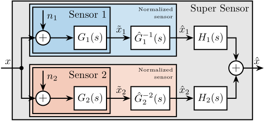
\end{tikzpicture}

Two normalized sensors are then combined to form a super sensor as shown in Figure ref:fig:detail_control_sensor_fusion_super_sensor. The two sensors measure the same physical quantity $x$ with dynamics $G_1(s)$ and $G_2(s)$, and with uncorrelated noises $n_1$ and $n_2$. The signals from both normalized sensors are fed into two complementary filters $H_1(s)$ and $H_2(s)$ and then combined to yield an estimate $\hat{x}$ of $x$. The super sensor output $\hat{x}$ is therefore described by eqref:eq:detail_control_sensor_comp_filter_estimate.

\begin{equation}\label{eq:detail_control_sensor_comp_filter_estimate} \hat{x} = \Big( H_1(s) \hat{G}_1^-1(s) G_1(s) + H_2(s) \hat{G}_2^-1(s) G_2(s) \Big) x + H_1(s) \hat{G}_1^-1(s) G_1(s) n_1 + H_2(s) \hat{G}_2^-1(s) G_2(s) n_2

\end{equation}

\tikzset{block/.default={0.8cm}{0.8cm}}
\tikzset{addb/.append style={scale=0.7}}
\tikzset{node distance=0.6}
\begin{tikzpicture}
  \node[branch] (x) at (0, 0);
  \node[addb, above right=0.8 and 0.5 of x](add1){};
  \node[addb, below right=0.8 and 0.5 of x](add2){};
  \node[block, right=0.8 of add1](G1){$G_1(s)$};
  \node[block, right=0.8 of add2](G2){$G_2(s)$};
  \node[block, right=0.8 of G1](G1inv){$\hat{G}_1^{-1}(s)$};
  \node[block, right=0.8 of G2](G2inv){$\hat{G}_2^{-2}(s)$};
  \node[block, right=0.8 of G1inv](H1){$H_1(s)$};
  \node[block, right=0.8 of G2inv](H2){$H_2(s)$};
  \node[addb, right=7 of x](add){};

  \draw[] ($(x)+(-0.7, 0)$) node[above right]{$x$} -- (x.center);
  \draw[->] (x.center) |- (add1.west);
  \draw[->] (x.center) |- (add2.west);
  \draw[<-] (add1.north) -- ++(0, 0.7)node[below right](n1){$n_1$};
  \draw[->] (add1.east) -- (G1.west);
  \draw[->] (G1.east) -- (G1inv.west) node[above left]{$\tilde{x}_1$};
  \draw[->] (G1inv.east) -- (H1.west) node[above left]{$\hat{x}_1$};
  \draw[<-] (add2.north) -- ++(0, 0.7)node[below right](n2){$n_2$};
  \draw[->] (add2.east) -- (G2.west);
  \draw[->] (G2.east) -- (G2inv.west) node[above left]{$\tilde{x}_2$};
  \draw[->] (G2inv.east) -- (H2.west) node[above left]{$\hat{x}_2$};
  \draw[->] (H1) -| (add.north);
  \draw[->] (H2) -| (add.south);
  \draw[->] (add.east) -- ++(0.7, 0) node[above left]{$\hat{x}$};

  \begin{scope}[on background layer]
    \node[fit={(G2.south-|x) (n1.north-|add.east)}, fill=black!10!white, draw, inner sep=9pt] (supersensor) {};
    \node[below left] at (supersensor.north east) {Super Sensor};

    \node[fit={(add1.west |- G1inv.south) (n1.north -| G1inv.east)}, fill=colorblue!20!white, draw, inner sep=6pt] (sensor1cal) {};
    \node[below left, align=right] at (sensor1cal.north east) {{\tiny Normalized}\\[-0.5em]{\tiny sensor}};
    \node[fit={(add1.west |- G1.south) (n1.north -| G1.east)}, fill=colorblue!30!white, draw, inner sep=3pt] (sensor1) {};
    \node[below left] at (sensor1.north east) {Sensor 1};

    \node[fit={(add2.west |- G2inv.south) (n2.north -| G2inv.east)}, fill=colorred!20!white, draw, inner sep=6pt] (sensor2cal) {};
    \node[below left, align=right] at (sensor2cal.north east) {{\tiny Normalized}\\[-0.5em]{\tiny sensor}};
    \node[fit={(add2.west |- G2.south) (n2.north -| G2.east)}, fill=colorred!30!white, draw, inner sep=3pt] (sensor2) {};
    \node[below left] at (sensor2.north east) {Sensor 2};
  \end{scope}
\end{tikzpicture}

Sensor fusion architecture with two normalized sensors.

Noise Sensor Filtering

First, consider the case where all sensors are perfectly normalized eqref:eq:detail_control_sensor_perfect_dynamics. The effects of imperfect normalization will be addressed subsequently.

\begin{equation}\label{eq:detail_control_sensor_perfect_dynamics} \frac{\hat{x}_i}{x} = \hat{G}_i(s) G_i(s) = 1

\end{equation}

In that case, the super sensor output $\hat{x}$ equals $x$ plus the filtered noise from both sensors eqref:eq:detail_control_sensor_estimate_perfect_dyn. From this equation, it is evident that the complementary filters $H_1(s)$ and $H_2(s)$ operate solely on the sensor noise. Thus, this sensor fusion architecture allows filtering of sensor noise without introducing distortion in the measured physical quantity. This fundamental property necessitates that the two filters must be complementary.

\begin{equation}\label{eq:detail_control_sensor_estimate_perfect_dyn} \hat{x} = x + H_1(s) n_1 + H_2(s) n_2

\end{equation}

The estimation error $\epsilon_x$, defined as the difference between the sensor output $\hat{x}$ and the measured quantity $x$, is computed for the super sensor eqref:eq:detail_control_sensor_estimate_error.

\begin{equation}\label{eq:detail_control_sensor_estimate_error} ε_x ≜ \hat{x} - x = H_1(s) n_1 + H_2(s) n_2

\end{equation}

As shown in eqref:eq:detail_control_sensor_noise_filtering_psd, the Power Spectral Density (PSD) of the estimation error $\Phi_{\epsilon_x}$ depends both on the norm of the two complementary filters and on the PSD of the noise sources $\Phi_{n_1}$ and $\Phi_{n_2}$.

\begin{equation}\label{eq:detail_control_sensor_noise_filtering_psd} Φ_{ε_x}(ω) = ≤ft|H_1(jω)\right|^2 Φ_{n_1}(ω) + ≤ft|H_2(jω)\right|^2 Φ_{n_2}(ω)

\end{equation}

If the two sensors have identical noise characteristics ($\Phi_{n_1}(\omega) = \Phi_{n_2}(\omega)$), simple averaging ($H_1(s) = H_2(s) = 0.5$) would minimize the super sensor noise. This represents the simplest form of sensor fusion using complementary filters.

However, sensors typically exhibit high noise levels in different frequency regions. In such cases, to reduce the noise of the super sensor, the norm $|H_1(j\omega)|$ should be minimized when $\Phi_{n_1}(\omega)$ exceeds $\Phi_{n_2}(\omega)$, and the norm $|H_2(j\omega)|$ should be minimized when $\Phi_{n_2}(\omega)$ exceeds $\Phi_{n_1}(\omega)$. Therefore, by appropriately shaping the norm of the complementary filters, the noise of the super sensor can be minimized.

Sensor Fusion Robustness

In practical systems, sensor normalization is rarely perfect, and condition eqref:eq:detail_control_sensor_perfect_dynamics is not fully satisfied.

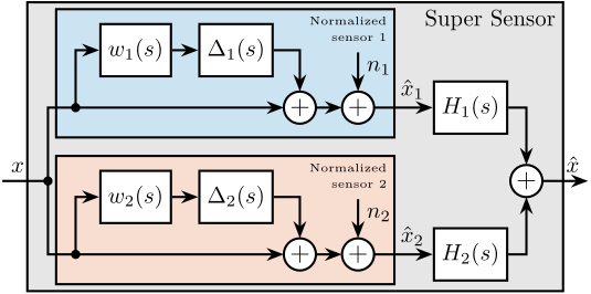
To analyze such imperfections, a multiplicative input uncertainty is incorporated into the sensor dynamics (Figure ref:fig:detail_control_sensor_model_uncertainty). The nominal model is the estimated model used for normalization $\hat{G}_i(s)$, $\Delta_i(s)$ is any stable transfer function satisfying $|\Delta_i(j\omega)| \le 1,\ \forall\omega$, and $w_i(s)$ is a weighting transfer function representing the magnitude of uncertainty. The weight $w_i(s)$ is selected such that the actual sensor dynamics $G_i(j\omega)$ remains within the uncertain region represented by a circle in the complex plane, centered on $1$ with a radius equal to $|w_i(j\omega)|$.

Since the nominal sensor dynamics is taken as the normalized filter, the normalized sensor model can be further simplified as shown in Figure ref:fig:detail_control_sensor_model_uncertainty_simplified.

\tikzset{block/.default={0.8cm}{0.8cm}}
\tikzset{addb/.append style={scale=0.7}}
\tikzset{node distance=0.6}
\begin{tikzpicture}
  \node[branch] (input) at (0,0) {};
  \node[block, above right= 0.4 and 0.4 of input](W1){$w_1(s)$};
  \node[block, right=0.4 of W1](delta1){$\Delta_1(s)$};
  \node[addb] (addu) at ($(delta1.east|-input) + (0.4, 0)$) {};
  \node[addb, right=0.4 of addu] (addn) {};
  \node[block, right=0.4 of addn] (G1) {$\hat{G}_1(s)$};
  \node[block, right=0.8 of G1](G1inv){$\hat{G}_1^{-1}(s)$};

  \draw[->] ($(input)+(-0.7, 0)$) node[above right]{$x$} -- (addu);
  \draw[->] (input.center) |- (W1.west);
  \draw[->] (W1.east) -- (delta1.west);
  \draw[->] (delta1.east) -| (addu.north);
  \draw[->] (addu.east) -- (addn.west);
  \draw[->] (addn.east) -- (G1.west);
  \draw[<-] (addn.north) -- ++(0, 0.7)node[below right](n1){$n_1$};
  \draw[->] (G1.east) -- (G1inv.west) node[above left]{$\tilde{x}_1$};
  \draw[->] (G1inv.east) -- ++(0.8, 0) node[above left]{$\hat{x}_1$};

  \begin{scope}[on background layer]
    \node[fit={(input.west |- G1inv.south) (delta1.north -| G1inv.east)}, fill=black!10!white, draw, inner sep=6pt] (sensor1cal) {};
    \node[below left, align=right] at (sensor1cal.north east) {{\tiny Normalized}\\[-0.5em]{\tiny sensor}};

    \node[fit={(input.west |- G1.south) (delta1.north -| G1.east)}, fill=black!20!white, draw, inner sep=3pt] (sensor1) {};
    \node[below left] at (sensor1.north east) {Sensor};
  \end{scope}
\end{tikzpicture}

\tikzset{block/.default={0.8cm}{0.8cm}}
\tikzset{addb/.append style={scale=0.7}}
\tikzset{node distance=0.6}
\begin{tikzpicture}
  \node[branch] (input) at (0,0) {};
  \node[block, above right= 0.4 and 0.4 of input](W1){$w_1(s)$};
  \node[block, right=0.4 of W1](delta1){$\Delta_1(s)$};
  \node[addb] (addu) at ($(delta1.east|-input) + (0.4, 0)$) {};
  \node[addb, right=0.4 of addu] (addn) {};

  \draw[->] ($(input)+(-0.8, 0)$) node[above right]{$x$} -- (addu);
  \draw[->] (input.center) |- (W1.west);
  \draw[->] (W1.east) -- (delta1.west);
  \draw[->] (delta1.east) -| (addu.north);
  \draw[->] (addu.east) -- (addn.west);
  \draw[<-] (addn.north) -- ++(0, 0.6)node[below right](n1){$n_1$};
  \draw[->] (addn.east) -- ++(0.9, 0) node[above left]{$\hat{x}_1$};

  \begin{scope}[on background layer]
    \node[fit={(input.west |- addu.south) ($(delta1.north -| addn.east) + (0.1, 0)$)}, fill=black!10!white, draw, inner sep=6pt] (sensor1cal) {};
    \node[below left, align=right] at (sensor1cal.north east) {{\tiny Normalized}\\[-0.5em]{\tiny sensor}};
  \end{scope}
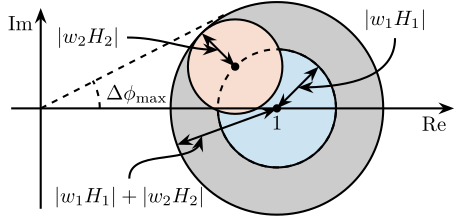
\end{tikzpicture}

The sensor fusion architecture incorporating sensor models with dynamical uncertainty is illustrated in Figure ref:fig:detail_control_sensor_fusion_dynamic_uncertainty. The super sensor dynamics eqref:eq:detail_control_sensor_super_sensor_dyn_uncertainty is no longer unity but depends on the sensor dynamical uncertainty weights $w_i(s)$ and the complementary filters $H_i(s)$. The dynamical uncertainty of the super sensor can be graphically represented in the complex plane by a circle centered on $1$ with a radius equal to $|w_1(j\omega) H_1(j\omega)| + |w_2(j\omega) H_2(j\omega)|$ (Figure ref:fig:detail_control_sensor_uncertainty_set_super_sensor).

The sensor fusion architecture with the sensor models including dynamical uncertainty is shown in Figure ref:fig:detail_control_sensor_fusion_dynamic_uncertainty. The super sensor dynamics eqref:eq:detail_control_sensor_super_sensor_dyn_uncertainty is no longer equal to $1$ and now depends on the sensor dynamical uncertainty weights $w_i(s)$ as well as on the complementary filters $H_i(s)$. The dynamical uncertainty of the super sensor can be graphically represented in the complex plane by a circle centered on $1$ with a radius equal to $|w_1(j\omega) H_1(j\omega)| + |w_2(j\omega) H_2(j\omega)|$ (Figure ref:fig:detail_control_sensor_uncertainty_set_super_sensor).

\begin{equation}\label{eq:detail_control_sensor_super_sensor_dyn_uncertainty} \frac{\hat{x}}{x} = 1 + w_1(s) H_1(s) Δ_1(s) + w_2(s) H_2(s) Δ_2(s)

\end{equation}

\tikzset{block/.default={0.8cm}{0.8cm}}
\tikzset{addb/.append style={scale=0.7}}
\tikzset{node distance=0.6}
\begin{tikzpicture}
  \node[branch] (x) at (0, 0);

  \node[branch, above right=1.0 and 0.3 of x] (input1) {};
  \node[branch, below right=1.0 and 0.3 of x] (input2) {};
  \node[block, above right= 0.4 and 0.3 of input1](W1){$w_1(s)$};
  \node[block, above right= 0.4 and 0.3 of input2](W2){$w_2(s)$};
  \node[block, right=0.4 of W1](delta1){$\Delta_1(s)$};
  \node[block, right=0.4 of W2](delta2){$\Delta_2(s)$};
  \node[addb] (addu1) at ($(delta1.east|-input1) + (0.4, 0)$) {};
  \node[addb] (addu2) at ($(delta2.east|-input2) + (0.4, 0)$) {};
  \node[addb, right=0.4 of addu1] (addn1) {};
  \node[addb, right=0.4 of addu2] (addn2) {};
  \node[block, right=0.9 of addn1](H1){$H_1(s)$};
  \node[block, right=0.9 of addn2](H2){$H_2(s)$};

  \node[addb, right=7 of x](add){};


  \draw[] ($(x)+(-0.7, 0)$) node[above right]{$x$} -- (x.center);
  \draw[->] (x.center) |- (addu1.west);
  \draw[->] (x.center) |- (addu2.west);
  \draw[->] (input1.center) |- (W1.west);
  \draw[->] (W1.east) -- (delta1.west);
  \draw[->] (delta1.east) -| (addu1.north);
  \draw[->] (addu1.east) -- (addn1.west);
  \draw[<-] (addn1.north) -- ++(0, 0.6)node[below right](n1){$n_1$};
  \draw[->] (input2.center) |- (W2.west);
  \draw[->] (W2.east) -- (delta2.west);
  \draw[->] (delta2.east) -| (addu2.north);
  \draw[->] (addu2.east) -- (addn2.west);
  \draw[<-] (addn2.north) -- ++(0, 0.6)node[below right](n2){$n_2$};

  \draw[->] (addn1.east) -- (H1.west) node[above left]{$\hat{x}_1$};
  \draw[->] (addn2.east) -- (H2.west) node[above left]{$\hat{x}_2$};
  \draw[->] (H1) -| (add.north);
  \draw[->] (H2) -| (add.south);
  \draw[->] (add.east) -- ++(0.7, 0) node[above left]{$\hat{x}$};

  \begin{scope}[on background layer]
    \node[fit={(addn2.south-|x) (delta1.north-|add.east)}, fill=black!10!white, draw, inner sep=9pt] (supersensor) {};
    \node[below left] at (supersensor.north east) {Super Sensor};

    \node[fit={(input1.west |- addu1.south) ($(delta1.north -| addn1.east) + (0.1, 0.0)$)}, fill=colorblue!20!white, draw, inner sep=6pt] (sensor1cal) {};
    \node[below left, align=right] at (sensor1cal.north east) {{\tiny Normalized}\\[-0.5em]{\tiny sensor 1}};

    \node[fit={(input2.west |- addu2.south) ($(delta2.north -| addn1.east) + (0.1, 0.0)$)}, fill=colorred!20!white, draw, inner sep=6pt] (sensor2cal) {};
    \node[below left, align=right] at (sensor2cal.north east) {{\tiny Normalized}\\[-0.5em]{\tiny sensor 2}};
  \end{scope}
\end{tikzpicture}

\tikzset{block/.default={0.8cm}{0.8cm}}
\tikzset{addb/.append style={scale=0.7}}
\tikzset{node distance=0.6}
\begin{tikzpicture}
  \begin{scope}[shift={(4, 0)}]

    % Uncertainty Circle
    \node[draw, circle, fill=black!20!white, minimum size=3.6cm] (c) at (0, 0) {};
    \path[draw, fill=colorblue!20!white] (0, 0) circle [radius=1.0];
    \path[draw, fill=colorred!20!white] (135:1.0) circle [radius=0.8];
    \path[draw, dashed] (0, 0) circle [radius=1.0];

    % Center of Circle
    \node[below] at (0, 0){$1$};

    \draw[<->] (0, 0)   node[branch]{} -- coordinate[midway](r1) ++(45:1.0);
    \draw[<->] (135:1.0)node[branch]{} -- coordinate[midway](r2) ++(135:0.8);

    \node[] (l1) at (2, 1.5) {$|w_1 H_1|$};
    \draw[->, out=-90, in=0] (l1.south) to (r1);

    \node[] (l2) at (-3.2, 1.2) {$|w_2 H_2|$};
    \draw[->, out=0, in=-180] (l2.east) to (r2);

    \draw[<->] (0, 0) -- coordinate[near end](r3) ++(200:1.8);
    \node[] (l3) at (-2.5, -1.5) {$|w_1 H_1| + |w_2 H_2|$};
    \draw[->, out=90, in=-90] (l3.north) to (r3);
  \end{scope}

  % Real and Imaginary Axis
  \draw[->] (-0.5, 0) -- (7.0, 0) node[below left]{Re};
  \draw[->] (0, -1.7) -- (0, 1.7) node[below left]{Im};

  \draw[dashed] (0, 0) -- (tangent cs:node=c,point={(0, 0)},solution=2);
  \draw[dashed] (1, 0) arc (0:28:1) node[midway, right]{$\Delta \phi_\text{max}$};
\end{tikzpicture}

The super sensor dynamical uncertainty, and consequently the robustness of the fusion, clearly depends on the complementary filters' norm. As it is generally desired to limit the dynamical uncertainty of the super sensor, the norm of the complementary filter $|H_i(j\omega)|$ should be made small when $|w_i(j\omega)|$ is large, i.e., at frequencies where the sensor dynamics is uncertain.

Complementary Filters Shaping

<<ssec:detail_control_sensor_hinf_method>>

Introduction   ignore

As established in Section ref:ssec:detail_control_sensor_fusion_requirements, the super sensor's noise characteristics and robustness are directly dependent on the complementary filters' norm. A synthesis method enabling precise shaping of these norms would therefore offer substantial practical benefits. This section develops such an approach by formulating the design objective as a standard $\mathcal{H}_\infty$ optimization problem. The methodology for designing appropriate weighting functions (which specify desired complementary filter shapes during synthesis) is examined in detail, and the efficacy of the proposed method is validated with a simple example.

Synthesis Objective

The primary objective is to shape the norms of two filters $H_1(s)$ and $H_2(s)$ while ensuring they maintain their complementary property as defined in eqref:eq:detail_control_sensor_comp_filter. This is equivalent to finding proper and stable transfer functions $H_1(s)$ and $H_2(s)$ that satisfy conditions eqref:eq:detail_control_sensor_hinf_cond_complementarity, eqref:eq:detail_control_sensor_hinf_cond_h1, and eqref:eq:detail_control_sensor_hinf_cond_h2. Weighting transfer functions $W_1(s)$ and $W_2(s)$ are strategically selected to define the maximum desired norm of the complementary filters during the synthesis process.

\begin{subequations}\label{eq:detail_control_sensor_comp_filter_problem_form}

\begin{align} & H_1(s) + H_2(s) = 1 \label{eq:detail_control_sensor_hinf_cond_complementarity} \\ & |H_1(j\omega)| \le \frac{1}{|W_1(j\omega)|} \quad \forall\omega \label{eq:detail_control_sensor_hinf_cond_h1} \\ & |H_2(j\omega)| \le \frac{1}{|W_2(j\omega)|} \quad \forall\omega \label{eq:detail_control_sensor_hinf_cond_h2} \end{align}

\end{subequations}

Shaping of Complementary Filters using $\mathcal{H}_\infty$ synthesis

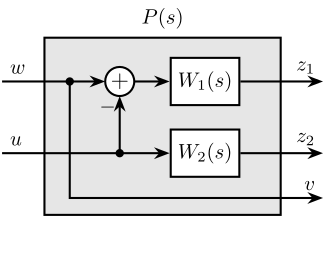
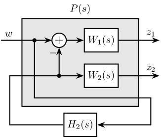
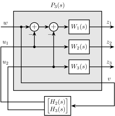
The synthesis objective can be readily expressed as a standard $\mathcal{H}_\infty$ optimization problem and solved using widely available computational tools. Consider the generalized plant $P(s)$ illustrated in Figure ref:fig:detail_control_sensor_h_infinity_robust_fusion_plant and mathematically described by eqref:eq:detail_control_sensor_generalized_plant.

\begin{equation}\label{eq:detail_control_sensor_generalized_plant} \begin{bmatrix} z_1 \\ z_2 \\ v \end{bmatrix} = P(s) \begin{bmatrix} w\\u \end{bmatrix}; \quad P(s) = \begin{bmatrix}W_1(s) & -W_1(s) \\ 0 & \phantom{+}W_2(s) \\ 1 & 0 \end{bmatrix} = P(s) \begin{bmatrix} w\\u \end{bmatrix}; \quad P(s) = \begin{bmatrix}W_1(s) & -W_1(s) \\ 0 & \phantom{+}W_2(s) \\ 1 & 0 \end{bmatrix}; \quad P(s) = \begin{bmatrix}W_1(s) & -W_1(s) \\ 0 & \phantom{+}W_2(s) \\ 1 & 0 \end{bmatrix}

\end{equation}

\tikzset{block/.default={0.8cm}{0.8cm}}
\tikzset{addb/.append style={scale=0.7}}
\tikzset{node distance=0.6}
\begin{tikzpicture}
  \node[block={4.0cm}{3.0cm}, fill=black!10!white] (P) {};
  \node[above] at (P.north) {$P(s)$};

  \node[block, below=0.2 of P, opacity=0] (H2) {$H_2(s)$};

  \coordinate[] (inputw)  at ($(P.south west)!0.75!(P.north west) + (-0.7, 0)$);
  \coordinate[] (inputu)  at ($(P.south west)!0.35!(P.north west) + (-0.7, 0)$);

  \coordinate[] (output1) at ($(P.south east)!0.75!(P.north east) + ( 0.7, 0)$);
  \coordinate[] (output2) at ($(P.south east)!0.35!(P.north east) + ( 0.7, 0)$);
  \coordinate[] (outputv) at ($(P.south east)!0.1!(P.north east) + ( 0.7, 0)$);

  \node[block, left=1.4 of output1] (W1){$W_1(s)$};
  \node[block, left=1.4 of output2] (W2){$W_2(s)$};
  \node[addb={+}{}{}{}{-}, left=of W1] (sub) {};

  \draw[->] (inputw) node[above right]{$w$} -- (sub.west);
  \draw[->] (inputu) node[above right]{$u$} -- (W2.west);
  \draw[->] (inputu-|sub) node[branch]{} -- (sub.south);
  \draw[->] (sub.east) -- (W1.west);
  \draw[->] ($(sub.west)+(-0.6, 0)$) node[branch]{} |- (outputv) node[above left]{$v$};
  \draw[->] (W1.east) -- (output1)node[above left]{$z_1$};
  \draw[->] (W2.east) -- (output2)node[above left]{$z_2$};
\end{tikzpicture}

\tikzset{block/.default={0.8cm}{0.8cm}}
\tikzset{addb/.append style={scale=0.7}}
\tikzset{node distance=0.6}
\begin{tikzpicture}
  \node[block={4.0cm}{3.0cm}, fill=black!10!white] (P) {};
  \node[above] at (P.north) {$P(s)$};

  \node[block, below=0.2 of P] (H2) {$H_2(s)$};

  \coordinate[] (inputw)  at ($(P.south west)!0.75!(P.north west) + (-0.7, 0)$);
  \coordinate[] (inputu)  at ($(P.south west)!0.35!(P.north west) + (-0.4, 0)$);

  \coordinate[] (output1) at ($(P.south east)!0.75!(P.north east) + ( 0.7, 0)$);
  \coordinate[] (output2) at ($(P.south east)!0.35!(P.north east) + ( 0.7, 0)$);
  \coordinate[] (outputv) at ($(P.south east)!0.1!(P.north east) + ( 0.4, 0)$);

  \node[block, left=1.4 of output1] (W1){$W_1(s)$};
  \node[block, left=1.4 of output2] (W2){$W_2(s)$};
  \node[addb={+}{}{}{}{-}, left=of W1] (sub) {};

  \draw[->] (inputw) node[above right]{$w$} -- (sub.west);
  \draw[->] (inputu-|sub) node[branch]{} -- (sub.south);
  \draw[->] (sub.east) -- (W1.west);
  \draw[->] ($(sub.west)+(-0.6, 0)$) node[branch]{} |- (outputv) |- (H2.east);
  \draw[->] (H2.west) -| (inputu) -- (W2.west);
  \draw[->] (W1.east) -- (output1)node[above left]{$z_1$};
  \draw[->] (W2.east) -- (output2)node[above left]{$z_2$};
\end{tikzpicture}

Applying standard $\mathcal{H}_\infty$ synthesis to the generalized plant $P(s)$ is equivalent to finding a stable filter $H_2(s)$ that, based on input $v$, generates an output signal $u$ such that the $\mathcal{H}_\infty$ norm of the system shown in Figure ref:fig:detail_control_sensor_h_infinity_robust_fusion_fb from $w$ to $[z_1, \ z_2]$ does not exceed unity, as expressed in eqref:eq:detail_control_sensor_hinf_syn_obj.

\begin{equation}\label{eq:detail_control_sensor_hinf_syn_obj} ≤ft\|\begin{matrix} \left(1 - H_2(s)\right) W_1(s) \\ H_2(s) W_2(s) \end{matrix}\right\|_∞ ≤ 1

\end{equation}

By defining $H_1(s)$ as the complement of $H_2(s)$ (eqref:eq:detail_control_sensor_definition_H1), the $\mathcal{H}_\infty$ synthesis objective becomes equivalent to eqref:eq:detail_control_sensor_hinf_problem, ensuring that conditions eqref:eq:detail_control_sensor_hinf_cond_h1 and eqref:eq:detail_control_sensor_hinf_cond_h2 are satisfied.

\begin{equation}\label{eq:detail_control_sensor_definition_H1} H_1(s) ≜ 1 - H_2(s)

\end{equation}

\begin{equation}\label{eq:detail_control_sensor_hinf_problem} ≤ft\|\begin{matrix} H_1(s) W_1(s) \\ H_2(s) W_2(s) \end{matrix}\right\|_∞ ≤ 1

\end{equation}

Therefore, applying $\mathcal{H}_\infty$ synthesis to the standard plant $P(s)$ (eqref:eq:detail_control_sensor_generalized_plant) generates two filters, $H_2(s)$ and $H_1(s) \triangleq 1 - H_2(s)$, that are complementary as required by eqref:eq:detail_control_sensor_comp_filter_problem_form, with norms bounded by the specified constraints in eqref:eq:detail_control_sensor_hinf_cond_h1 and eqref:eq:detail_control_sensor_hinf_cond_h2.

It should be noted that there exists only an implication (not an equivalence) between the $\mathcal{H}_\infty$ norm condition in eqref:eq:detail_control_sensor_hinf_problem and the initial synthesis objectives in eqref:eq:detail_control_sensor_hinf_cond_h1 and eqref:eq:detail_control_sensor_hinf_cond_h2. Consequently, the optimization may be somewhat conservative with respect to the set of filters on which it operates (see cite:&skogestad07_multiv_feedb_contr,Chap. 2.8.3).

Weighting Functions Design

Weighting functions play a crucial role during synthesis by specifying the maximum allowable norms for the complementary filters. The proper design of these weighting functions is essential for the successful implementation of the proposed $\mathcal{H}_\infty$ synthesis approach.

Three key considerations should guide the design of weighting functions. First, only proper and stable transfer functions should be employed. Second, the order of the weighting functions should remain reasonably small to minimize computational costs associated with solving the optimization problem and to facilitate practical implementation of the filters (as the order of the synthesized filters equals the sum of the weighting functions' orders). Third, the fundamental limitations imposed by the complementary property (eqref:eq:detail_control_sensor_comp_filter) must be respected, which implies that $|H_1(j\omega)|$ and $|H_2(j\omega)|$ cannot both be made small at the same frequency.

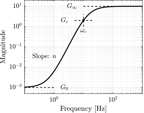
When designing complementary filters, it is typically desirable to specify their slopes, "blending" frequency, and maximum gains at low and high frequencies. To facilitate the expression of these specifications, formula eqref:eq:detail_control_sensor_weight_formula is proposed for the design of weighting functions. The parameters in this formula are $G_0 = \lim_{\omega \to 0} |W(j\omega)|$ (the low-frequency gain), $G_\infty = \lim_{\omega \to \infty} |W(j\omega)|$ (the high-frequency gain), $G_c = |W(j\omega_c)|$ (the gain at a specific frequency $\omega_c$ in $\si{rad/s}$), and $n$ (the slope between high and low frequency, which also corresponds to the order of the weighting function). The typical magnitude response of a weighting function generated using eqref:eq:detail_control_sensor_weight_formula is illustrated in Figure ref:fig:detail_control_sensor_weight_formula.

\hfill

\begin{equation}\label{eq:detail_control_sensor_weight_formula} W(s) = ≤ft( \frac{ \hfill{} \frac{1}{ω_c} \sqrt{\frac{1 - ≤ft(\frac{G_0}{G_c}\right)^{\frac{2}{n}}}{1 - ≤ft(\frac{G_c}{G_∞}\right)^{\frac{2}{n}}}} s + ≤ft(\frac{G_0}{G_c}\right)^{\frac{1}{n}} }{ ≤ft(\frac{1}{G_∞}\right)^{\frac{1}{n}} \frac{1}{ω_c} \sqrt{\frac{1 - ≤ft(\frac{G_0}{G_c}\right)^{\frac{2}{n}}}{1 - ≤ft(\frac{G_c}{G_∞}\right)^{\frac{2}{n}}}} s + ≤ft(\frac{1}{G_c}\right)^{\frac{1}{n}} }\right)^n

\end{equation}

Validation of the proposed synthesis method

The proposed methodology for designing complementary filters is now applied to a simple example. Consider the design of two complementary filters $H_1(s)$ and $H_2(s)$ with the following requirements:

• The blending frequency should be approximately $\SI{10}{Hz}$
• The slope of $|H_1(j\omega)|$ should be $+2$ below $\SI{10}{Hz}$, with a low-frequency gain of $10^{-3}$
• The slope of $|H_2(j\omega)|$ should be $-3$ above $\SI{10}{Hz}$, with a high-frequency gain of $10^{-3}$

The first step involves translating these requirements by appropriately designing the weighting functions. The formula proposed in eqref:eq:detail_control_sensor_weight_formula is employed for this purpose. The parameters used are summarized in Table ref:tab:detail_control_sensor_weights_params. The inverse magnitudes of the designed weighting functions, which represent the maximum allowable norms of the complementary filters, are depicted by the dashed lines in Figure ref:fig:detail_control_sensor_hinf_filters_results.

%% Synthesis of Complementary Filters using H-infinity synthesis
% Design of the Weighting Functions
W1 = generateWF('n', 3, 'w0', 2*pi*10, 'G0', 1000, 'Ginf', 1/10, 'Gc', 0.45);
W2 = generateWF('n', 2, 'w0', 2*pi*10, 'G0', 1/10, 'Ginf', 1000, 'Gc', 0.45);

% Generalized Plant
P = [W1 -W1;
     0   W2;
     1   0];

% H-Infinity Synthesis
[H2, ~, gamma, ~] = hinfsyn(P, 1, 1,'TOLGAM', 0.001, 'METHOD', 'ric', 'DISPLAY', 'on');

% Define H1 to be the complementary of H2
H1 = 1 - H2;

% The function generateCF can also be used to synthesize the complementary filters.
% [H1, H2] = generateCF(W1, W2);

Parameter	$W_1(s)$	$W_2(s)$
$G_0$	$0.1$	$1000$
$G_{\infty}$	$1000$	$0.1$
$\omega_c$	$2 \pi \cdot 10$	$2 \pi \cdot 10$
$G_c$	$0.45$	$0.45$
$n$	$2$	$3$

\hfill

Weights and obtained filters

Standard $\mathcal{H}_\infty$ synthesis is then applied to the generalized plant shown in Figure ref:fig:detail_control_sensor_h_infinity_robust_fusion_plant. This yields the filter $H_2(s)$ that minimizes the $\mathcal{H}_\infty$ norm from input $w$ to outputs $[z_1,\ z_2]^{\intercal}$. The resulting $\mathcal{H}_\infty$ norm is found to be close to unity, indicating successful synthesis: the norms of the complementary filters remain below the specified upper bounds. This is confirmed by the Bode plots of the obtained complementary filters in Figure ref:fig:detail_control_sensor_hinf_filters_results. This straightforward example demonstrates that the proposed methodology for shaping complementary filters is both simple and effective.

Synthesis of a set of three complementary filters

<<ssec:detail_control_sensor_hinf_three_comp_filters>>

Certain applications necessitate the fusion of more than two sensors cite:&stoten01_fusion_kinet_data_using_compos_filter;&fonseca15_compl. At LIGO, for example, a super sensor is formed by merging three distinct sensors: an LVDT, a seismometer, and a geophone cite:&matichard15_seism_isolat_advan_ligo.

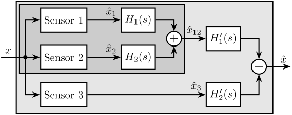
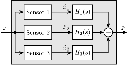
For merging $n>2$ sensors with complementary filters, two architectural approaches are possible, as illustrated in Figure ref:fig:detail_control_sensor_fusion_three. Fusion can be implemented either "sequentially," utilizing $n-1$ sets of two complementary filters (Figure ref:fig:detail_control_sensor_fusion_three_sequential), or "in parallel," employing a single set of $n$ complementary filters (Figure ref:fig:detail_control_sensor_fusion_three_parallel).

While conventional sensor fusion synthesis techniques can be applied to the sequential approach, parallel architecture implementation requires a novel synthesis method for multiple complementary filters. Previous literature has offered only simple analytical formulas for this purpose cite:&stoten01_fusion_kinet_data_using_compos_filter;&fonseca15_compl. This section presents a generalization of the proposed complementary filter synthesis method to address this gap.

\tikzset{block/.default={0.8cm}{0.8cm}}
\tikzset{addb/.append style={scale=0.7}}
\tikzset{node distance=0.6}
\begin{tikzpicture}
  \node[branch] (x) at (0, 0);

  \node[block, right=0.4 of x] (sensor2) {Sensor 2};
  \node[block, above=0.4 of sensor2] (sensor1) {Sensor 1};
  \node[block, below=0.4 of sensor2] (sensor3) {Sensor 3};

  \node[block, right=1.1 of sensor1](H1){$H_1(s)$};
  \node[block, right=1.1 of sensor2](H2){$H_2(s)$};
  \node[addb] (add) at ($0.5*(H1.east)+0.5*(H2.east)+(0.6, 0)$){};

  \node[block, right=0.8 of add](H1p)  {$H_1^\prime(s)$};
  \node[block] (H2p) at (H1p|-sensor3) {$H_2^\prime(s)$};

  \node[addb] (addp) at ($0.5*(H1p.east)+0.5*(H2p.east)+(0.6, 0)$){};

  \draw[->] ($(x)+(-0.8, 0)$) node[above right]{$x$} -- (sensor2.west);
  \draw[->] (x.center)     |- (sensor1.west);
  \draw[->] (x.center)     |- (sensor3.west);
  \draw[->] (sensor1.east) -- (H1.west)  node[above left]{$\hat{x}_1$};
  \draw[->] (sensor2.east) -- (H2.west)  node[above left]{$\hat{x}_2$};
  \draw[->] (sensor3.east) -- (H2p.west) node[above left]{$\hat{x}_3$};
  \draw[->] (H1)           -| (add.north);
  \draw[->] (H2)           -| (add.south);
  \draw[->] (add.east)     -- (H1p.west) node[above left]{$\hat{x}_{12}$};
  \draw[->] (H1p)          -| (addp.north);
  \draw[->] (H2p)          -| (addp.south);
  \draw[->] (addp.east)    -- ++(0.8, 0) node[above left]{$\hat{x}$};

  \begin{scope}[on background layer]
    \node[fit={(x.west|-sensor3.south) (sensor1.north-|addp.east)}, fill=black!10!white, draw, inner sep=6pt] (supersensor) {};

    \node[fit={(x.west|-sensor1.north) (add.east|-sensor2.south)}, fill=black!20!white, draw, inner sep=3pt] (superinertialsensor) {};
  \end{scope}
\end{tikzpicture}

\tikzset{block/.default={0.8cm}{0.8cm}}
\tikzset{addb/.append style={scale=0.7}}
\tikzset{node distance=0.6}
\begin{tikzpicture}
  \node[branch] (x) at (0, 0);
  \node[block, right=0.4 of x] (sensor2) {Sensor 2};
  \node[block, above=0.3 of sensor2] (sensor1) {Sensor 1};
  \node[block, below=0.3 of sensor2] (sensor3) {Sensor 3};

  \node[block, right=1.1 of sensor1](H1){$H_1(s)$};
  \node[block, right=1.1 of sensor2](H2){$H_2(s)$};
  \node[block, right=1.1 of sensor3](H3){$H_3(s)$};

  \node[addb, right=0.6 of H2](add){};

  \draw[->] (x.center)                             |- (sensor1.west);
  \draw[] ($(x)+(-0.8, 0)$) node[above right]{$x$} -- (sensor2.west);
  \draw[->] (x.center)                             |- (sensor3.west);

  \draw[->] (sensor1.east) -- (H1.west) node[above left]{$\hat{x}_1$};
  \draw[->] (sensor2.east) -- (H2.west) node[above left]{$\hat{x}_2$};
  \draw[->] (sensor3.east) -- (H3.west) node[above left]{$\hat{x}_3$};

  \draw[->] (H1) -| (add.north);
  \draw[->] (H2) -- (add.west);
  \draw[->] (H3) -| (add.south);

  \draw[->] (add.east) -- ++(0.8, 0) node[above left]{$\hat{x}$};

  \begin{scope}[on background layer]
    \node[fit={(H3.south-|x) (H1.north-|add.east)}, fill=black!10!white, draw, inner sep=6pt] (supersensor) {};
  \end{scope}
\end{tikzpicture}

The synthesis objective is to compute a set of $n$ stable transfer functions $[H_1(s),\ H_2(s),\ \dots,\ H_n(s)]$ that satisfy conditions eqref:eq:detail_control_sensor_hinf_cond_compl_gen and eqref:eq:detail_control_sensor_hinf_cond_perf_gen.

\begin{subequations}\label{eq:detail_control_sensor_hinf_problem_gen}

\begin{align} & \sum_{i=1}^n H_i(s) = 1 \label{eq:detail_control_sensor_hinf_cond_compl_gen} \\ & \left| H_i(j\omega) \right| < \frac{1}{\left| W_i(j\omega) \right|}, \quad \forall \omega,\ i = 1 \dots n \label{eq:detail_control_sensor_hinf_cond_perf_gen} \end{align}

\end{subequations}

The transfer functions $[W_1(s),\ W_2(s),\ \dots,\ W_n(s)]$ are weights selected to specify the maximum complementary filters' norm during synthesis.

This synthesis objective is closely related to the one described in Section ref:ssec:detail_control_sensor_hinf_method, and the proposed synthesis method represents a generalization of the approach previously presented. A set of $n$ complementary filters can be shaped by applying standard $\mathcal{H}_\infty$ synthesis to the generalized plant $P_n(s)$ described by eqref:eq:detail_control_sensor_generalized_plant_n_filters.

\begin{equation}\label{eq:detail_control_sensor_generalized_plant_n_filters} \begin{bmatrix} z_1 \\ \vdots \\ z_n \\ v \end{bmatrix} = P_n(s) \begin{bmatrix} w \\ u_1 \\ \vdots \\ u_{n-1} \end{bmatrix} = P_n(s) \begin{bmatrix} w \\ u_1 \\ \vdots \\ u_{n-1} \end{bmatrix}; \quad P_n(s) = \begin{bmatrix} W_1 & -W_1 & … & … & -W_1
0 & W_2 & 0 & … & 0
\vdots & \ddots & \ddots & \ddots & \vdots
\vdots & & \ddots & \ddots & 0
0 & … & … & 0 & W_n
1 & 0 & … & … & 0

\end{bmatrix}

\end{equation}

If the synthesis is successful, a set of $n-1$ filters $[H_2(s),\ H_3(s),\ \dots,\ H_n(s)]$ is obtained such that eqref:eq:detail_control_sensor_hinf_syn_obj_gen is satisfied.

\begin{equation}\label{eq:detail_control_sensor_hinf_syn_obj_gen} ≤ft\|\begin{matrix} \left(1 - \left[ H_2(s) + H_3(s) + \dots + H_n(s) \right]\right) W_1(s) \\ H_2(s) W_2(s) \\ \vdots \\ H_n(s) W_n(s) \end{matrix}\right\|_∞ ≤ 1

\end{equation}

$H_1(s)$ is then defined using eqref:eq:detail_control_sensor_h1_comp_h2_hn, which ensures the complementary property for the set of $n$ filters eqref:eq:detail_control_sensor_hinf_cond_compl_gen. Condition eqref:eq:detail_control_sensor_hinf_cond_perf_gen is satisfied through eqref:eq:detail_control_sensor_hinf_syn_obj_gen.

\begin{equation}\label{eq:detail_control_sensor_h1_comp_h2_hn} H_1(s) ≜ 1 - \big[ H_2(s) + H_3(s) + … + H_n(s) \big]

\end{equation}

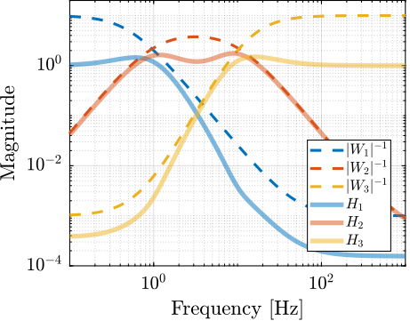
To validate the proposed method for synthesizing a set of three complementary filters, an example is provided. The sensors to be merged are a displacement sensor (effective from DC up to $\SI{1}{Hz}$), a geophone (effective from $1$ to $\SI{10}{Hz}$), and an accelerometer (effective above $\SI{10}{Hz}$). Three weighting functions are designed using formula eqref:eq:detail_control_sensor_weight_formula, and their inverse magnitudes are shown in Figure ref:fig:detail_control_sensor_three_complementary_filters_results (dashed curves).

Consider the generalized plant $P_3(s)$ shown in Figure ref:fig:detail_control_sensor_comp_filter_three_hinf_fb, which is also described by eqref:eq:detail_control_sensor_generalized_plant_three_filters.

\begin{equation}\label{eq:detail_control_sensor_generalized_plant_three_filters} \begin{bmatrix} z_1 \\ z_2 \\ z_3 \\ v \end{bmatrix} = P_3(s) \begin{bmatrix} w \\ u_1 \\ u_2 \end{bmatrix}; \quad P_3(s) = \begin{bmatrix}W_1(s) & -W_1(s) & -W_1(s) \\ 0 & \phantom{+}W_2(s) & 0 \\ 0 & 0 & \phantom{+}W_3(s) \\ 1 & 0 & 0 \end{bmatrix} = P_3(s) \begin{bmatrix} w \\ u_1 \\ u_2 \end{bmatrix}; \quad P_3(s) = \begin{bmatrix}W_1(s) & -W_1(s) & -W_1(s) \\ 0 & \phantom{+}W_2(s) & 0 \\ 0 & 0 & \phantom{+}W_3(s) \\ 1 & 0 & 0 \end{bmatrix}; \quad P_3(s) = \begin{bmatrix}W_1(s) & -W_1(s) & -W_1(s) \\ 0 & \phantom{+}W_2(s) & 0 \\ 0 & 0 & \phantom{+}W_3(s) \\ 1 & 0 & 0 \end{bmatrix}

\end{equation}

\tikzset{block/.default={0.8cm}{0.8cm}}
\tikzset{addb/.append style={scale=0.7}}
\tikzset{node distance=0.6}
\begin{tikzpicture}
  \node[block={5.0cm}{4.5cm}, fill=black!10!white] (P) {};
  \node[above] at (P.north) {$P_3(s)$};

  \coordinate[] (inputw)  at ($(P.south west)!0.8!(P.north west) + (-0.7, 0)$);
  \coordinate[] (inputu)  at ($(P.south west)!0.4!(P.north west) + (-0.7, 0)$);

  \coordinate[] (output1) at ($(P.south east)!0.8!(P.north east)  + (0.7, 0)$);
  \coordinate[] (output2) at ($(P.south east)!0.55!(P.north east) + (0.7, 0)$);
  \coordinate[] (output3) at ($(P.south east)!0.3!(P.north east)  + (0.7, 0)$);
  \coordinate[] (outputv) at ($(P.south east)!0.1!(P.north east)  + (0.7, 0)$);

  \node[block, left=1.4 of output1] (W1){$W_1(s)$};
  \node[block, left=1.4 of output2] (W2){$W_2(s)$};
  \node[block, left=1.4 of output3] (W3){$W_3(s)$};
  \node[addb={+}{}{}{}{-}, left=of W1] (sub1) {};
  \node[addb={+}{}{}{}{-}, left=of sub1] (sub2) {};

  \node[block, below=0.3 of P, opacity=0] (H) {$\begin{bmatrix}H_2(s) \\ H_3(s)\end{bmatrix}$};

  \draw[->] (inputw) node[above right](w){$w$} -- (sub2.west);
  \draw[->] (W3-|sub1)node[branch]{} -- (sub1.south);
  \draw[->] (W2-|sub2)node[branch]{} -- (sub2.south);
  \draw[->] ($(sub2.west)+(-0.5, 0)$) node[branch]{} |- (outputv);
  \draw[->] (inputu|-W2) -- (W2.west);
  \draw[->] (inputu|-W3) -- (W3.west);

  \draw[->] (sub2.east) -- (sub1.west);
  \draw[->] (sub1.east) -- (W1.west);
  \draw[->] (W1.east) -- (output1)node[above left](z){$z_1$};
  \draw[->] (W2.east) -- (output2)node[above left]{$z_2$};
  \draw[->] (W3.east) -- (output3)node[above left]{$z_3$};
  \node[above] at (W2-|w){$u_1$};
  \node[above] at (W3-|w){$u_2$};
  \node[above] at (outputv-|z){$v$};
\end{tikzpicture}

\tikzset{block/.default={0.8cm}{0.8cm}}
\tikzset{addb/.append style={scale=0.7}}
\tikzset{node distance=0.6}
\begin{tikzpicture}
  \node[block={5.0cm}{4.5cm}, fill=black!10!white] (P) {};
  \node[above] at (P.north) {$P_3(s)$};

  \coordinate[] (inputw)  at ($(P.south west)!0.8!(P.north west) + (-0.7, 0)$);
  \coordinate[] (inputu)  at ($(P.south west)!0.4!(P.north west) + (-0.7, 0)$);

  \coordinate[] (output1) at ($(P.south east)!0.8!(P.north east)  + (0.7, 0)$);
  \coordinate[] (output2) at ($(P.south east)!0.55!(P.north east) + (0.7, 0)$);
  \coordinate[] (output3) at ($(P.south east)!0.3!(P.north east)  + (0.7, 0)$);
  \coordinate[] (outputv) at ($(P.south east)!0.1!(P.north east)  + (0.7, 0)$);

  \node[block, left=1.4 of output1] (W1){$W_1(s)$};
  \node[block, left=1.4 of output2] (W2){$W_2(s)$};
  \node[block, left=1.4 of output3] (W3){$W_3(s)$};
  \node[addb={+}{}{}{}{-}, left=of W1] (sub1) {};
  \node[addb={+}{}{}{}{-}, left=of sub1] (sub2) {};

  \node[block, below=0.3 of P] (H) {$\begin{bmatrix}H_2(s) \\ H_3(s)\end{bmatrix}$};

  \draw[->] (inputw) node[above right](w){$w$} -- (sub2.west);
  \draw[->] (W3-|sub1)node[branch]{} -- (sub1.south);
  \draw[->] (W2-|sub2)node[branch]{} -- (sub2.south);
  \draw[->] ($(sub2.west)+(-0.5, 0)$) node[branch]{} |- (outputv) |- (H.east);
  \draw[->] ($(H.south west)!0.7!(H.north west)$) -| (inputu|-W2) -- (W2.west);
  \draw[->] ($(H.south west)!0.3!(H.north west)$) -| ($(inputu|-W3)+(0.4, 0)$) -- (W3.west);

  \draw[->] (sub2.east) -- (sub1.west);
  \draw[->] (sub1.east) -- (W1.west);
  \draw[->] (W1.east) -- (output1)node[above left](z){$z_1$};
  \draw[->] (W2.east) -- (output2)node[above left]{$z_2$};
  \draw[->] (W3.east) -- (output3)node[above left]{$z_3$};
  \node[above] at (W2-|w){$u_1$};
  \node[above] at (W3-|w){$u_2$};
  \node[above] at (outputv-|z){$v$};
\end{tikzpicture}

Standard $\mathcal{H}_\infty$ synthesis is performed on the generalized plant $P_3(s)$. Two filters, $H_2(s)$ and $H_3(s)$, are obtained such that the $\mathcal{H}_\infty$ norm of the closed-loop transfer from $w$ to $[z_1,\ z_2,\ z_3]$ of the system in Figure ref:fig:detail_control_sensor_comp_filter_three_hinf_fb is less than one. Filter $H_1(s)$ is defined using eqref:eq:detail_control_sensor_h1_compl_h2_h3, thus ensuring the complementary property of the obtained set of filters.

\begin{equation}\label{eq:detail_control_sensor_h1_compl_h2_h3} H_1(s) ≜ 1 - \big[ H_2(s) + H_3(s) \big]

\end{equation}

Figure ref:fig:detail_control_sensor_three_complementary_filters_results displays the three synthesized complementary filters (solid lines), confirming the successful synthesis.

%% Synthesis of a set of three complementary filters
% Design of the Weighting Functions
W1 = generateWF('n', 2, 'w0', 2*pi*1, 'G0', 1/10, 'Ginf', 1000, 'Gc', 0.5);
W2 = 0.22*(1 + s/2/pi/1)^2/(sqrt(1e-4) + s/2/pi/1)^2*(1 + s/2/pi/10)^2/(1 + s/2/pi/1000)^2;
W3 = generateWF('n', 3, 'w0', 2*pi*10, 'G0', 1000, 'Ginf', 1/10, 'Gc', 0.5);

% Generalized plant for the synthesis of 3 complementary filters
P = [W1 -W1 -W1;
     0   W2  0 ;
     0   0   W3;
     1   0   0];

% Standard H-Infinity Synthesis
[H, ~, gamma, ~] = hinfsyn(P, 1, 2,'TOLGAM', 0.001, 'METHOD', 'ric', 'DISPLAY', 'on');

% Synthesized H2 and H3 filters
H2 = tf(H(1));
H3 = tf(H(2));

% H1 is defined as the complementary filter of H2 and H3
H1 = 1 - H2 - H3;

Conclusion

A new method for designing complementary filters using the $\mathcal{H}_\infty$ synthesis has been proposed. This approach allows shaping of the filter magnitudes through the use of weighting functions during synthesis. This capability is particularly valuable in practice since the characteristics of the super sensor are directly linked to the complementary filters' magnitude. Consequently, typical sensor fusion objectives can be effectively translated into requirements on the magnitudes of the filters.

For the Nano Active Stabilization System (NASS), the High Authority Control-Integral Force Feedback (HAC-IFF) strategy was found to perform well and to offer the advantages of being both intuitive to understand and straightforward to tune. Looking forward, it would be interesting to investigate how sensor fusion (particularly between the force sensor and external metrology) compares to the HAC-IFF approach in terms of performance and robustness.

Decoupling

<<sec:detail_control_decoupling>>

Introduction   ignore

The control of parallel manipulators (and any MIMO system in general) typically involves a two-step approach: first decoupling the plant dynamics using various strategies, which will be discussed in this section, followed by the application of SISO control for the decoupled plant (discussed in section ref:sec:detail_control_cf).

When sensors are integrated within the struts, decentralized control may be applied, as the system is already well decoupled at low frequency. For instance, cite:&furutani04_nanom_cuttin_machin_using_stewar implemented a system where each strut consists of piezoelectric stack actuators and eddy current displacement sensors, with separate PI controllers for each strut. A similar control architecture was proposed in cite:&du14_piezo_actuat_high_precis_flexib using strain gauge sensors integrated in each strut.

An alternative strategy involves decoupling the system in the Cartesian frame using Jacobian matrices. As demonstrated during the study of Stewart platform kinematics, Jacobian matrices can be utilized to map actuator forces to forces and torques applied on the top platform. This approach enables the implementation of controllers in a defined frame. It has been applied with various sensor types including force sensors cite:&mcinroy00_desig_contr_flexur_joint_hexap, relative displacement sensors cite:&kim00_robus_track_contr_desig_dof_paral_manip, and inertial sensors cite:&li01_simul_vibrat_isolat_point_contr;&abbas14_vibrat_stewar_platf. The Cartesian frame in which the system is decoupled is typically chosen at the point of interest (i.e., where the motion is of interest) or at the center of mass.

Modal control represents another noteworthy decoupling strategy, wherein the "local" plant inputs and outputs are mapped to the modal space. In this approach, multiple SISO plants, each corresponding to a single mode, can be controlled independently. This decoupling strategy has been implemented for active damping applications cite:&holterman05_activ_dampin_based_decoup_colloc_contr, which is logical as it is often desirable to dampen specific modes. The strategy has also been employed in cite:&pu11_six_degree_of_freed_activ for vibration isolation purposes using geophones, and in cite:&yang19_dynam_model_decoup_contr_flexib using force sensors.

Another completely different strategy, is to use implement a multivariable control directly on the coupled system. $\mathcal{H}_\infty$ and $\mu\text{-synthesis}$ were applied to a Stewart platform model in cite:&lei08_multi_objec_robus_activ_vibrat. In cite:&xie17_model_contr_hybrid_passiv_activ, decentralized force feedback was first applied, followed by $\mathcal{H}_2$ synthesis for vibration isolation based on accelerometers. $\mathcal{H}_\infty$ synthesis was also employed in cite:&jiao18_dynam_model_exper_analy_stewar for active damping based on accelerometers. cite:&thayer02_six_axis_vibrat_isolat_system compared $\mathcal{H}_\infty$ synthesis with decentralized control in the frame of the struts. Their experimental closed-loop results indicated that the $\mathcal{H}_\infty$ controller did not outperform the decentralized controller in the frame of the struts. These limitations were attributed to the model's poor ability to predict off-diagonal dynamics, which is crucial for $\mathcal{H}_\infty$ synthesis.

The purpose of this section is to compare several methods for the decoupling of parallel manipulators, an analysis that appears to be lacking in the literature. The analysis begins in Section ref:ssec:detail_control_decoupling_model with the introduction of a simplified parallel manipulator model that serves as the foundation for evaluating various decoupling strategies. Sections ref:ssec:detail_control_decoupling_jacobian through ref:ssec:detail_control_decoupling_svd systematically examine three distinct approaches: Jacobian matrix decoupling, modal decoupling, and Singular Value Decomposition (SVD) decoupling, respectively. The comparative assessment of these three methodologies, along with concluding observations, is provided in Section ref:ssec:detail_control_decoupling_comp.

Test Model

<<ssec:detail_control_decoupling_model>>

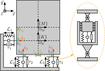
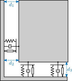
Instead of utilizing the Stewart platform for comparing decoupling strategies, a simplified parallel manipulator is employed to facilitate a more straightforward analysis. The system illustrated in Figure ref:fig:detail_control_decoupling_model_test is used for this purpose. It possesses three degrees of freedom (DoF) and incorporates three parallel struts. Being a fully parallel manipulator, it is therefore quite similar to the Stewart platform.

Two reference frames are defined within this model: frame $\{M\}$ with origin $O_M$ at the center of mass of the solid body, and frame $\{K\}$ with origin $O_K$ at the center of stiffness of the parallel manipulator.

\hfill

	Description	Value
$l_a$		$0.5\,m$
$h_a$		$0.2\,m$
$k$	Actuator stiffness	$10\,N/\mu m$
$c$	Actuator damping	$200\,Ns/m$
$m$	Payload mass	$40\,\text{kg}$
$I$	Payload $R_z$ inertia	$5\,\text{kg}m^2$

The equations of motion are derived by applying Newton's second law to the suspended mass, expressed at its center of mass eqref:eq:detail_control_decoupling_model_eom, where $\bm{\mathcal{X}}_{\{M\}}$ represents the two translations and one rotation with respect to the center of mass, and $\bm{\mathcal{F}}_{\{M\}}$ denotes the forces and torque applied at the center of mass.

\begin{equation}\label{eq:detail_control_decoupling_model_eom} \bm{M}_{\{M\}} \ddot{\bm{\mathcal{X}}}_{\{M\}}(t) = ∑ \bm{\mathcal{F}}_{\{M\}}(t), \quad \bm{\mathcal{X}}_{\{M\}} = \begin{bmatrix} x \\ y \\ R_z \end{bmatrix}, \quad \bm{\mathcal{F}}_{\{M\}} = \begin{bmatrix} F_x
F_y
M_z

\end{bmatrix}

\end{equation}

The Jacobian matrix $\bm{J}_{\{M\}}$ is employed to map the spring, damping, and actuator forces to XY forces and Z torque expressed at the center of mass eqref:eq:detail_control_decoupling_jacobian_CoM.

\begin{equation}\label{eq:detail_control_decoupling_jacobian_CoM} \bm{J}_{\{M\}} = \begin{bmatrix} 1 & 0 & h_a
0 & 1 & -l_a
0 & 1 & l_a \\

\end{bmatrix}

\end{equation}

Subsequently, the equation of motion relating the actuator forces $\tau$ to the motion of the mass $\bm{\mathcal{X}}_{\{M\}}$ is derived eqref:eq:detail_control_decoupling_plant_cartesian.

\begin{equation}\label{eq:detail_control_decoupling_plant_cartesian} \bm{M}_{\{M\}} \ddot{\bm{\mathcal{X}}}_{\{M\}}(t) + \bm{J}_{\{M\}}^∫ercal \bm{\mathcal{C}} \bm{J}_{\{M\}} \dot{\bm{\mathcal{X}}}_{\{M\}}(t) + \bm{J}_{\{M\}}^∫ercal \bm{\mathcal{K}} \bm{J}_{\{M\}} \bm{\mathcal{X}}_{\{M\}}(t) = \bm{J}_{\{M\}}^∫ercal \bm{τ}(t)

\end{equation}

The matrices representing the payload inertia, actuator stiffness, and damping are shown in eqref:eq:detail_control_decoupling_system_matrices.

\begin{equation}\label{eq:detail_control_decoupling_system_matrices} \bm{M}_{\{M\}} = \begin{bmatrix} m & 0 & 0 \\ 0 & m & 0 \\ 0 & 0 & I \end{bmatrix}, \quad \bm{\mathcal{K}} = \begin{bmatrix} k & 0 & 0 \\ 0 & k & 0 \\ 0 & 0 & k \end{bmatrix}, \quad \bm{\mathcal{K}} = \begin{bmatrix} k & 0 & 0 \\ 0 & k & 0 \\ 0 & 0 & k \end{bmatrix}, \quad \bm{\mathcal{C}} = \begin{bmatrix} c & 0 & 0
0 & c & 0
0 & 0 & c

\end{bmatrix}

\end{equation}

The parameters employed for the subsequent analysis are summarized in Table ref:tab:detail_control_decoupling_test_model_params, which includes values for geometric parameters ($l_a$, $h_a$), mechanical properties (actuator stiffness $k$ and damping $c$), and inertial characteristics (payload mass $m$ and rotational inertia $I$).

Control in the frame of the struts

<<ssec:detail_control_decoupling_decentralized>>

The dynamics in the frame of the struts are first examined. The equation of motion relating actuator forces $\bm{\mathcal{\tau}}$ to strut relative motion $\bm{\mathcal{L}}$ is derived from equation eqref:eq:detail_control_decoupling_plant_cartesian by mapping the Cartesian motion of the mass to the relative motion of the struts using the Jacobian matrix $\bm{J}_{\{M\}}$ defined in eqref:eq:detail_control_decoupling_jacobian_CoM. The obtained transfer function from $\bm{\mathcal{\tau}}$ to $\bm{\mathcal{L}}$ is shown in eqref:eq:detail_control_decoupling_plant_decentralized.

\begin{tikzpicture}
  \node[block] (Gl) {$\bm{G}_{\{\mathcal{L}\}}$};

  % Connections and labels
  \draw[<-] (Gl.west) -- ++(-0.8, 0) node[above right]{$\bm{\tau}$};
  \draw[->] (Gl.east) -- ++( 0.8, 0) node[above left]{$\bm{\mathcal{L}}$};
\end{tikzpicture}

\begin{equation}\label{eq:detail_control_decoupling_plant_decentralized} \frac{\bm{\mathcal{L}}}{\bm{\mathcal{τ}}}(s) = \bm{G}_{\mathcal{L}}(s) = ≤ft( \bm{J}_{\{M\}}^-∫ercal \bm{M}_{\{M\}} \bm{J}_{\{M\}}^-1 s^2 + \bm{\mathcal{C}} s + \bm{\mathcal{K}} \right)^-1

\end{equation}

At low frequencies, the plant converges to a diagonal constant matrix whose diagonal elements are related to the actuator stiffnesses eqref:eq:detail_control_decoupling_plant_decentralized_low_freq. At high frequencies, the plant converges to the mass matrix mapped in the frame of the struts, which is generally highly non-diagonal.

\begin{equation}\label{eq:detail_control_decoupling_plant_decentralized_low_freq} \bm{G}_{\mathcal{L}}(jω) \xrightarrow[ω → 0]{} \bm{\mathcal{K}^-1}

\end{equation}

%% Compute Equation of motion
l = 1; h=2;
la = 0.5; % Horizontal position of actuators [m]
ha = 0.2; % Vertical of actuators [m]

m = 40; % Payload mass [kg]
I = 5; % Payload rotational inertia [kg m^2]

c = 2e2; % Actuator Damping [N/(m/s)]
k = 1e6; % Actuator Stiffness [N/m]

% Unit vectors of the actuators
s1 = [1;0];
s2 = [0;1];
s3 = [0;1];

% Stiffnesss and Damping matrices of the struts
Kr = diag([k,k,k]);
Cr = diag([c,c,c]);

%  Location of the joints with respect to the center of mass
Mb1 = [-l/2;-ha];
Mb2 = [-la; -h/2];
Mb3 = [ la; -h/2];

% Jacobian matrix (Center of Mass)
J_CoM = [s1', Mb1(1)*s1(2)-Mb1(2)*s1(1);
         s2', Mb2(1)*s2(2)-Mb2(2)*s2(1);
         s3', Mb3(1)*s3(2)-Mb3(2)*s3(1)];

% Mass Matrix in frame {M}
M = diag([m,m,I]);

% Stiffness Matrix in frame {M}
K = J_CoM'*Kr*J_CoM;

% Damping Matrix in frame {M}
C = J_CoM'*Cr*J_CoM;

% Plant in the frame of the struts
G_L = J_CoM*inv(M*s^2 + C*s + K)*J_CoM';

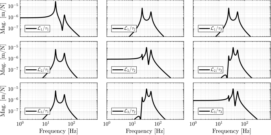
The magnitude of the coupled plant $\bm{G}_{\mathcal{L}}$ is illustrated in Figure ref:fig:detail_control_decoupling_coupled_plant_bode. This representation confirms that at low frequencies (below the first suspension mode), the plant is well decoupled. Depending on the symmetry present in the system, certain diagonal elements may exhibit identical values, as demonstrated for struts 2 and 3 in this example.

Model dynamics from actuator forces to relative displacement sensor of each strut.

Jacobian Decoupling

<<ssec:detail_control_decoupling_jacobian>>

Jacobian Matrix

The Jacobian matrix serves a dual purpose in the decoupling process: it converts strut velocity $\dot{\mathcal{L}}$ to payload velocity and angular velocity $\dot{\bm{\mathcal{X}}}_{\{O\}}$, and it transforms actuator forces $\bm{\tau}$ to forces/torque applied on the payload $\bm{\mathcal{F}}_{\{O\}}$, as expressed in equation eqref:eq:detail_control_decoupling_jacobian.

\begin{subequations}\label{eq:detail_control_decoupling_jacobian}

\begin{align} \dot{\bm{\mathcal{X}}}_{\{O\}} &= \bm{J}_{\{O\}} \dot{\bm{\mathcal{L}}}, \quad \dot{\bm{\mathcal{L}}} = \bm{J}_{\{O\}}^{-1} \dot{\bm{\mathcal{X}}}_{\{O\}} \\ \bm{\mathcal{F}}_{\{O\}} &= \bm{J}_{\{O\}}^{\intercal} \bm{\tau}, \quad \bm{\tau} = \bm{J}_{\{O\}}^{-\intercal} \bm{\mathcal{F}}_{\{O\}} \end{align}

\end{subequations}

The resulting plant (Figure ref:fig:detail_control_jacobian_decoupling_arch) have inputs and outputs with clear physical interpretations:

• $\bm{\mathcal{F}}_{\{O\}}$ represents forces/torques applied on the payload at the origin of frame $\{O\}$
• $\bm{\mathcal{X}}_{\{O\}}$ represents translations/rotation of the payload expressed in frame $\{O\}$

\begin{tikzpicture}
  \node[block] (G) {$\bm{G}_{\{\mathcal{L}\}}$};
  \node[block, left=0.6 of G] (Jt) {$\bm{J}_{\{O\}}^{-\intercal}$};
  \node[block, right=0.6 of G] (Ja) {$\bm{J}_{\{O\}}^{-1}$};

  % Connections and labels
  \draw[<-] (Jt.west) -- ++(-1.4, 0) node[above right]{$\bm{\mathcal{F}}_{\{O\}}$};
  \draw[->] (Jt.east) -- (G.west)  node[above left]{$\bm{\tau}$};
  \draw[->] (G.east) -- (Ja.west)  node[above left]{$\bm{\mathcal{L}}$};
  \draw[->] (Ja.east) -- ++( 1.4, 0)  node[above left]{$\bm{\mathcal{X}}_{\{O\}}$};

  \begin{scope}[on background layer]
    \node[fit={(Jt.south west) (Ja.north east)}, fill=black!10!white, draw, dashed, inner sep=4pt] (Gx) {};
    \node[above] at (Gx.north) {$\bm{G}_{\{O\}}$};
  \end{scope}
\end{tikzpicture}

Block diagram of the transfer function from $\bm{\mathcal{F}}_{\{O\}}$ to $\bm{\mathcal{X}}_{\{O\}}$

The transfer function from $\bm{\mathcal{F}}_{\{O\}$ to $\bm{\mathcal{X}}_{\{O\}}$, denoted $\bm{G}_{\{O\}}(s)$ can be computed using eqref:eq:detail_control_decoupling_plant_jacobian.

\begin{equation}\label{eq:detail_control_decoupling_plant_jacobian} \frac{\bm{\mathcal{X}}_{\{O\}}}{\bm{\mathcal{F}}_{\{O\}}}(s) = \bm{G}_{\{O\}}(s) = ≤ft( \bm{J}_{\{O\}}^∫ercal \bm{J}_{\{M\}}^-∫ercal \bm{M}_{\{M\}} \bm{J}_{\{M\}}^-1 \bm{J}_{\{O\}} s^2 + \bm{J}_{\{O\}}^∫ercal \bm{\mathcal{C}} \bm{J}_{\{O\}} s + \bm{J}_{\{O\}}^∫ercal \bm{\mathcal{K}} \bm{J}_{\{O\}} \right)^-1

\end{equation}

The frame $\{O\}$ can be selected according to specific requirements, but the decoupling properties are significantly influenced by this choice. Two natural reference frames are particularly relevant: the center of mass and the center of stiffness.

Center Of Mass

When the decoupling frame is located at the center of mass (frame $\{M\}$ in Figure ref:fig:detail_control_decoupling_model_test), the Jacobian matrix and its inverse are expressed as in eqref:eq:detail_control_decoupling_jacobian_CoM_inverse.

\begin{equation}\label{eq:detail_control_decoupling_jacobian_CoM_inverse} \bm{J}_{\{M\}} = \begin{bmatrix} 1 & 0 & h_a \\ 0 & 1 & -l_a \\ 0 & 1 & l_a \\ \end{bmatrix}, \quad \bm{J}_{\{M\}}^-1 = \begin{bmatrix} 1 & \frac{h_a}{2 l_a} & \frac{-h_a}{2 l_a}
0 & \frac{1}{2} & \frac{1}{2}
0 & \frac{-1}{2 l_a} & \frac{1}{2 l_a} \\

\end{bmatrix}

\end{equation}

\begin{tikzpicture}
  \node[block] (G) {$\bm{G}_{\{\mathcal{L}\}}$};
  \node[block, left=0.6 of G] (Jt) {$\bm{J}_{\{M\}}^{-\intercal}$};
  \node[block, right=0.6 of G] (Ja) {$\bm{J}_{\{M\}}^{-1}$};

  % Connections and labels
  \draw[<-] (Jt.west) -- ++(-1.4, 0) node[above right]{$\bm{\mathcal{F}}_{\{M\}}$};
  \draw[->] (Jt.east) -- (G.west)  node[above left]{$\bm{\tau}$};
  \draw[->] (G.east) -- (Ja.west)  node[above left]{$\bm{\mathcal{L}}$};
  \draw[->] (Ja.east) -- ++( 1.4, 0)  node[above left]{$\bm{\mathcal{X}}_{\{M\}}$};

  \begin{scope}[on background layer]
    \node[fit={(Jt.south west) (Ja.north east)}, fill=black!10!white, draw, dashed, inner sep=4pt] (Gx) {};
    \node[above] at (Gx.north) {$\bm{G}_{\{M\}}$};
  \end{scope}
\end{tikzpicture}

Analytical formula of the plant $\bm{G}_{\{M\}}(s)$ is derived eqref:eq:detail_control_decoupling_plant_CoM.

\begin{equation}\label{eq:detail_control_decoupling_plant_CoM} \frac{\bm{\mathcal{X}}_{\{M\}}}{\bm{\mathcal{F}}_{\{M\}}}(s) = \bm{G}_{\{M\}}(s) = ≤ft( \bm{M}_{\{M\}} s^2 + \bm{J}_{\{M\}}^∫ercal \bm{\mathcal{C}} \bm{J}_{\{M\}} s + \bm{J}_{\{M\}}^∫ercal \bm{\mathcal{K}} \bm{J}_{\{M\}} \right)^-1

\end{equation}

At high frequencies, the plant converges to the inverse of the mass matrix, which is a diagonal matrix eqref:eq:detail_control_decoupling_plant_CoM_high_freq.

\begin{equation}\label{eq:detail_control_decoupling_plant_CoM_high_freq} \bm{G}_{\{M\}}(jω) \xrightarrow[ω → ∞]{} -ω^2 \bm{M}_{\{M\}}^-1 = -ω^2 \begin{bmatrix} 1/m & 0 & 0
0 & 1/m & 0
0 & 0 & 1/I

\end{bmatrix}

\end{equation}

Consequently, the plant exhibits effective decoupling at frequencies above the highest suspension mode as shown in Figure ref:fig:detail_control_decoupling_jacobian_plant_CoM. This strategy is typically employed in systems with low-frequency suspension modes cite:&butler11_posit_contr_lithog_equip, where the plant approximates decoupled mass lines.

The low-frequency coupling observed in this configuration has a clear physical interpretation. When a static force is applied at the center of mass, the suspended mass rotates around the center of stiffness. This rotation is due to torque induced by the stiffness of the first actuator (i.e. the one on the left side), which is not aligned with the force application point. This phenomenon is illustrated in Figure ref:fig:detail_control_decoupling_model_test_CoM.

%% Jacobian Decoupling - Center of Mass
G_CoM = pinv(J_CoM)*G_L*pinv(J_CoM');
G_CoM.InputName  = {'Fx', 'Fy', 'Mz'};
G_CoM.OutputName  = {'Dx', 'Dy', 'Rz'};

Center Of Stiffness

\begin{tikzpicture}
  \node[block] (G) {$\bm{G}_{\{\mathcal{L}\}}$};
  \node[block, left=0.6 of G] (Jt) {$\bm{J}_{\{K\}}^{-\intercal}$};
  \node[block, right=0.6 of G] (Ja) {$\bm{J}_{\{K\}}^{-1}$};

  % Connections and labels
  \draw[<-] (Jt.west) -- ++(-1.4, 0) node[above right]{$\bm{\mathcal{F}}_{\{K\}}$};
  \draw[->] (Jt.east) -- (G.west)  node[above left]{$\bm{\tau}$};
  \draw[->] (G.east) -- (Ja.west)  node[above left]{$\bm{\mathcal{L}}$};
  \draw[->] (Ja.east) -- ++( 1.4, 0)  node[above left]{$\bm{\mathcal{X}}_{\{K\}}$};

  \begin{scope}[on background layer]
    \node[fit={(Jt.south west) (Ja.north east)}, fill=black!10!white, draw, dashed, inner sep=4pt] (Gx) {};
    \node[above] at (Gx.north) {$\bm{G}_{\{K\}}$};
  \end{scope}
\end{tikzpicture}

When the decoupling frame is located at the center of stiffness, the Jacobian matrix and its inverse are expressed as in eqref:eq:detail_control_decoupling_jacobian_CoK_inverse.

\begin{equation}\label{eq:detail_control_decoupling_jacobian_CoK_inverse} \bm{J}_{\{K\}} = \begin{bmatrix} 1 & 0 & 0 \\ 0 & 1 & -l_a \\ 0 & 1 & l_a \end{bmatrix}, \quad \bm{J}_{\{K\}}^-1 = \begin{bmatrix} 1 & 0 & 0
0 & \frac{1}{2} & \frac{1}{2}
0 & \frac{-1}{2 l_a} & \frac{1}{2 l_a}

\end{bmatrix}

\end{equation}

The frame $\{K\}$ was selected based on physical reasoning, positioned in line with the side strut and equidistant between the two vertical struts. However, it could alternatively be determined through analytical methods to ensure that $\bm{J}_{\{K\}}^{\intercal} \bm{\mathcal{K}} \bm{J}_{\{K\}}$ forms a diagonal matrix. It should be noted that the existence of such a center of stiffness (i.e. a frame $\{K\}$ for which $\bm{J}_{\{K\}}^{\intercal} \bm{\mathcal{K}} \bm{J}_{\{K\}}$ is diagonal) is not guaranteed for arbitrary systems. This property is typically achievable only in systems exhibiting specific symmetrical characteristics, as is the case in the present example.

The analytical expression for the plant in this configuration was then computed ref:eq:detail_control_decoupling_plant_CoK.

\begin{equation}\label{eq:detail_control_decoupling_plant_CoK} \frac{\bm{\mathcal{X}}_{\{K\}}}{\bm{\mathcal{F}}_{\{K\}}}(s) = \bm{G}_{\{K\}}(s) = ≤ft( \bm{J}_{\{K\}}^∫ercal \bm{J}_{\{M\}}^-∫ercal \bm{M}_{\{M\}} \bm{J}_{\{M\}}^-1 \bm{J}_{\{K\}} s^2 + \bm{J}_{\{K\}}^∫ercal \bm{\mathcal{C}} \bm{J}_{\{K\}} s + \bm{J}_{\{K\}}^∫ercal \bm{\mathcal{K}} \bm{J}_{\{K\}} \right)^-1

\end{equation}

Figure ref:fig:detail_control_decoupling_jacobian_plant_CoK_results presents the dynamics of the plant when decoupled using the Jacobian matrix expressed at the center of stiffness. The plant is well decoupled below the suspension mode with the lowest frequency eqref:eq:detail_control_decoupling_plant_CoK_low_freq, making it particularly suitable for systems with high stiffness.

\begin{equation}\label{eq:detail_control_decoupling_plant_CoK_low_freq} \bm{G}_{\{K\}}(jω) \xrightarrow[ω → 0]{} \bm{J}_{\{K\}}^-1 \bm{\mathcal{K}}^-1 \bm{J}_{\{K\}}^-∫ercal

\end{equation}

The physical reason for high-frequency coupling is illustrated in Figure ref:fig:detail_control_decoupling_model_test_CoK. When a high-frequency force is applied at a point not aligned with the center of mass, it induces rotation around the center of mass. This phenomenon explains the coupling observed between different degrees of freedom at higher frequencies.

%% Jacobian Decoupling - Center of Mass
%  Location of the joints with respect to the center of stiffness
Mb1 = [-l/2; 0];
Mb2 = [-la; -h/2+ha];
Mb3 = [ la; -h/2+ha];

% Jacobian matrix (Center of Stiffness)
J_CoK = [s1', Mb1(1)*s1(2)-Mb1(2)*s1(1);
         s2', Mb2(1)*s2(2)-Mb2(2)*s2(1);
         s3', Mb3(1)*s3(2)-Mb3(2)*s3(1)];

G_CoK = pinv(J_CoK)*G_L*pinv(J_CoK');
G_CoK.InputName   = {'Fx', 'Fy', 'Mz'};
G_CoK.OutputName  = {'Dx', 'Dy', 'Rz'};

Modal Decoupling

<<ssec:detail_control_decoupling_modal>>

Theory   ignore

Modal decoupling represents an approach based on the principle that a mechanical system's behavior can be understood as a combination of contributions from various modes cite:&rankers98_machin.

To convert the dynamics in the modal space, the equation of motion are first written with respect to the center of mass eqref:eq:detail_control_decoupling_equation_motion_CoM.

\begin{equation}\label{eq:detail_control_decoupling_equation_motion_CoM} \bm{M}_{\{M\}} \ddot{\bm{\mathcal{X}}}_{\{M\}}(t) + \bm{C}_{\{M\}} \dot{\bm{\mathcal{X}}}_{\{M\}}(t) + \bm{K}_{\{M\}} \bm{\mathcal{X}}_{\{M\}}(t) = \bm{J}_{\{M\}}^∫ercal \bm{τ}(t)

\end{equation}

For modal decoupling, a change of variables is introduced eqref:eq:detail_control_decoupling_modal_coordinates where $\bm{\mathcal{X}}_{m}$ represents the modal amplitudes and $\bm{\Phi}$ is a $n \times n$² matrix whose columns correspond to the mode shapes of the system, computed from $\bm{M}_{\{M\}}$ and $\bm{K}_{\{M\}}$.

\begin{equation}\label{eq:detail_control_decoupling_modal_coordinates} \bm{\mathcal{X}}_{\{M\}} = \bm{Φ} \bm{\mathcal{X}}_m

\end{equation}

By pre-multiplying equation eqref:eq:detail_control_decoupling_equation_motion_CoM by $\bm{\Phi}^{\intercal}$ and applying the change of variable eqref:eq:detail_control_decoupling_modal_coordinates, a new set of equations of motion is obtained eqref:eq:detail_control_decoupling_equation_modal_coordinates where $\bm{\tau}_m$ represents the modal input, while $\bm{M}_m$, $\bm{C}_m$, and $\bm{K}_m$ denote the modal mass, damping, and stiffness matrices respectively.

\begin{equation}\label{eq:detail_control_decoupling_equation_modal_coordinates} _brace{\bm{Φ}^∫ercal \bm{M} \bm{Φ}}_{\bm{M}_m} \bm{\ddot{\mathcal{X}}}_m(t) + _brace{\bm{Φ}^∫ercal \bm{C} \bm{Φ}}_{\bm{C}_m} \bm{\dot{\mathcal{X}}}_m(t) + _brace{\bm{Φ}^∫ercal \bm{K} \bm{Φ}}_{\bm{K}_m} \bm{\mathcal{X}}_m(t) = _brace{\bm{Φ}^∫ercal \bm{J}^∫ercal \bm{τ}(t)}_{\bm{τ}_m(t)}

\end{equation} The inherent mathematical structure of the mass, damping, and stiffness matrices cite:&lang17_under, chapt. 8 ensures that modal matrices are diagonal cite:&preumont18_vibrat_contr_activ_struc_fourt_edition, chapt. 2.3. This diagonalization transforms equation eqref:eq:detail_control_decoupling_equation_modal_coordinates into a set of $n$ decoupled equations, enabling independent control of each mode without cross-interaction.

To implement this approach from a decentralized plant, the architecture shown in Figure ref:fig:detail_control_decoupling_modal is employed. Inputs of the decoupling plant are the modal modal inputs $\bm{\tau}_m$ and the outputs are the modal amplitudes $\bm{\mathcal{X}}_m$. This implementation requires knowledge of the system's equations of motion, from which the mode shapes matrix $\bm{\Phi}$ is derived. The resulting decoupled system features diagonal elements each representing second-order resonant systems that are straightforward to control individually.

\begin{tikzpicture}
  \node[block] (G) {$\bm{G}_{\{\mathcal{L}\}}$};
  \node[block, left=0.6 of G] (Jt) {$\bm{J}_{\{M\}}^{-\intercal}$};
  \node[block, left=1.2 of Jt] (Bm) {$\bm{\Phi}^{-\intercal}$};
  \node[block, right=0.6 of G] (J) {$\bm{J}_{\{M\}}^{-1}$};
  \node[block, right=1.2 of J] (Cm) {$\bm{\Phi}^{-1}$};

  % Connections and labels
  \draw[<-] (Bm.west) -- ++(-1.0, 0) node[above right]{$\bm{\tau}_m$};
  \draw[->] (Bm.east) -- (Jt.west)  node[above left]{$\bm{\mathcal{F}}_{\{M\}}$};
  \draw[->] (Jt.east) -- (G.west)  node[above left]{$\bm{\tau}$};
  \draw[->] (G.east) -- (J.west)  node[above left]{$\bm{\mathcal{L}}$};
  \draw[->] (J.east) -- (Cm.west)  node[above left]{$\bm{\mathcal{X}}_{\{M\}}$};
  \draw[->] (Cm.east) -- ++( 1.0, 0)  node[above left]{$\bm{\mathcal{X}}_m$};

  \begin{scope}[on background layer]
    \node[fit={(Bm.south west) (Cm.north east)}, fill=black!10!white, draw, dashed, inner sep=4pt] (Gm) {};
    \node[above] at (Gm.north) {$\bm{G}_m$};
  \end{scope}
\end{tikzpicture}

Modal Decoupling Architecture

Example   ignore

Modal decoupling was then applied to the test model. First, the eigenvectors $\bm{\Phi}$ of $\bm{M}_{\{M\}}^{-1}\bm{K}_{\{M\}}$ were computed eqref:eq:detail_control_decoupling_modal_eigenvectors. While analytical derivation of eigenvectors could be obtained for such a simple system, they are typically computed numerically for practical applications.

\begin{equation}\label{eq:detail_control_decoupling_modal_eigenvectors} \bm{Φ} = \begin{bmatrix} \frac{I - h_a^2 m - 2 l_a^2 m - \alpha}{2 h_a m} & 0 & \frac{I - h_a^2 m - 2 l_a^2 m + \alpha}{2 h_a m} \\ 0 & 1 & 0 \\ 1 & 0 & 1 \end{bmatrix},\ α = \sqrt{≤ft( I + m (h_a^2 - 2 l_a^2) \right)^2 + 8 m^2 h_a^2 l_a^2}

\end{equation}

The numerical values for the eigenvector matrix and its inverse are shown in eqref:eq:detail_control_decoupling_modal_eigenvectors_matrices.

\begin{equation}\label{eq:detail_control_decoupling_modal_eigenvectors_matrices} \bm{Φ} = \begin{bmatrix} -0.905 & 0 & -0.058 \\ 0 & 1 & 0 \\ 0.424 & 0 & -0.998 \end{bmatrix}, \quad \bm{Φ}^-1 = \begin{bmatrix} -1.075 & 0 & 0.063
0 & 1 & 0
-0.457 & 0 & -0.975

\end{bmatrix}

\end{equation}

The two computed matrices were implemented in the control architecture of Figure ref:fig:detail_control_decoupling_modal, resulting in three distinct second order plants as depicted in Figure ref:fig:detail_control_decoupling_modal_plant. Each of these diagonal elements corresponds to a specific mode, as shown in Figure ref:fig:detail_control_decoupling_model_test_modal, resulting in a perfectly decoupled system.

%% Modal decoupling
% Compute the eigen vectors
[phi, wi] = eig(M\K);
% Sort the eigen vectors by increasing associated frequency
[~, i] = sort(diag(wi));
phi = phi(:, i);

% Plant in the modal space
Gm = inv(phi)*inv(J_CoM)*G_L*inv(J_CoM')*inv(phi');

SVD Decoupling

<<ssec:detail_control_decoupling_svd>>

Singular Value Decomposition

Singular Value Decomposition (SVD) represents a powerful mathematical tool with extensive applications in data analysis cite:&brunton22_data, chapt. 1 and multivariable control systems cite:&skogestad07_multiv_feedb_contr, where it is particularly valuable for analyzing directional properties in multivariable systems.

The SVD constitutes a unique matrix decomposition applicable to any complex matrix $\bm{X} \in \mathbb{C}^{n \times m}$, expressed as:

\begin{equation}\label{eq:detail_control_svd} \bm{X} = \bm{U} \bm{Σ} \bm{V}^H

\end{equation}

where $\bm{U} \in \mathbb{C}^{n \times n}$ and $\bm{V} \in \mathbb{C}^{m \times m}$ are unitary matrices with orthonormal columns, and $\bm{\Sigma} \in \mathbb{R}^{n \times n}$ is a diagonal matrix with real, non-negative entries. For real matrices $\bm{X}$, the resulting $\bm{U}$ and $\bm{V}$ matrices are also real, making them suitable for decoupling applications.

Decoupling using the SVD

The procedure for SVD-based decoupling begins with identifying the system dynamics from inputs to outputs, typically represented as a Frequency Response Function (FRF), which yields a complex matrix $\bm{G}(\omega_i)$ for multiple frequency points $\omega_i$. A specific frequency is then selected for optimal decoupling, with the targeted crossover frequency $\omega_c$ often serving as an appropriate choice.

Since real matrices are required for the decoupling transformation, a real approximation of the complex measured response at the selected frequency must be computed. In this work, the method proposed in cite:&kouvaritakis79_theor_pract_charac_locus_desig_method was used as it preserves maximal orthogonality in the directional properties of the input complex matrix.

Following this approximation, a real matrix $\tilde{\bm{G}}(\omega_c)$ is obtained, and SVD is performed on this matrix. The resulting (real) unitary matrices $\bm{U}$ and $\bm{V}$ are structured such that $\bm{V}^{-\intercal} \tilde{\bm{G}}(\omega_c) \bm{U}^{-1}$ forms a diagonal matrix. These singular input and output matrices are then applied to decouple the system as illustrated in Figure ref:fig:detail_control_decoupling_svd, and the decoupled plant is described by eqref:eq:detail_control_decoupling_plant_svd.

\begin{equation}\label{eq:detail_control_decoupling_plant_svd} \bm{G}_{\text{SVD}}(s) = \bm{U}^-1 \bm{G}_{\{\mathcal{L}\}}(s) \bm{V}^-∫ercal

\end{equation}

\begin{tikzpicture}
  \node[block] (G) {$\bm{G}_{\{\mathcal{L}\}}$};
  \node[block, left=0.6 of G.west] (V) {$\bm{V}^{-\intercal}$};
  \node[block, right=0.6 of G.east] (U) {$\bm{U}^{-1}$};

  % Connections and labels
  \draw[<-] (V.west) -- ++(-0.8, 0) node[above right]{$\bm{u}$};
  \draw[->] (V.east) -- (G.west) node[above left]{$\bm{\tau}$};
  \draw[->] (G.east) -- (U.west) node[above left]{$\bm{\mathcal{L}}$};
  \draw[->] (U.east) -- ++( 0.8, 0) node[above left]{$\bm{y}$};

  \begin{scope}[on background layer]
    \node[fit={(V.south west) (G.north-|U.east)}, fill=black!10!white, draw, dashed, inner sep=4pt] (Gsvd) {};
    \node[above] at (Gsvd.north) {$\bm{G}_{\text{SVD}}$};
  \end{scope}
\end{tikzpicture}

Decoupled plant $\bm{G}_{\text{SVD}}$ using the Singular Value Decomposition

Implementation of SVD decoupling requires access to the system's FRF, at least in the vicinity of the desired decoupling frequency. This information can be obtained either experimentally or derived from a model. While this approach ensures effective decoupling near the chosen frequency, it provides no guarantees regarding decoupling performance away from this frequency. Furthermore, the quality of decoupling depends significantly on the accuracy of the real approximation, potentially limiting its effectiveness for plants with high damping.

Example

Plant decoupling using the Singular Value Decomposition was then applied on the test model. A decoupling frequency of $\SI{100}{Hz}$ was used. The plant response at that frequency, as well as its real approximation and the obtained $\bm{U}$ and $\bm{V}$ matrices are shown in eqref:eq:detail_control_decoupling_svd_example.

\begin{equation}\label{eq:detail_control_decoupling_svd_example}

\begin{align} & \bm{G}_{\{\mathcal{L}\}}(\omega_c = 2\pi \cdot 100) = 10^{-9} \begin{bmatrix} -99 - j 2.6 & 74 + j 4.2 & -74 - j 4.2 \\ 74 + j 4.2 & -247 - j 9.7 & 102 + j 7.0 \\ -74 - j 4.2 & 102 + j 7.0 & -247 - j 9.7 \end{bmatrix} \\ & \xrightarrow[\text{approximation}]{\text{real}} \tilde{\bm{G}}_{\{\mathcal{L}\}}(\omega_c) = 10^{-9} \begin{bmatrix} -99 & 74 & -74 \\ 74 & -247 & 102 \\ -74 & 102 & -247 \end{bmatrix} \\ & \xrightarrow[\text{SVD}]{\phantom{\text{approximation}}} \bm{U} = \begin{bmatrix} 0.34 & 0 & 0.94 \\ -0.66 & 0.71 & 0.24 \\ 0.66 & 0.71 & -0.24 \end{bmatrix}, \ \bm{V} = \begin{bmatrix} -0.34 & 0 & -0.94 \\ 0.66 & -0.71 & -0.24 \\ -0.66 & -0.71 & 0.24 \end{bmatrix} \end{align}

\end{equation}

Using these $\bm{U}$ and $\bm{V}$ matrices, the decoupled plant is computed according to equation eqref:eq:detail_control_decoupling_plant_svd. The resulting plant, depicted in Figure ref:fig:detail_control_decoupling_svd_plant, exhibits remarkable decoupling across a broad frequency range, extending well beyond the vicinity of $\omega_c$. Additionally, the diagonal terms manifest as second-order dynamic systems, facilitating straightforward controller design.

%% SVD Decoupling
wc = 2*pi*100; % Decoupling frequency [rad/s]
% System's response at the decoupling frequency
H1 = evalfr(G_L, j*wc);

% Real approximation of G(j.wc)
D = pinv(real(H1'*H1));
H1 = pinv(D*real(H1'*diag(exp(j*angle(diag(H1*D*H1.'))/2))));

[U,S,V] = svd(H1);

Gsvd = inv(U)*G_L*inv(V');

Plant dynamics $\bm{G}_{\text{SVD}}(s)$ obtained after decoupling using Singular Value Decomposition

As it was surprising to obtain such a good decoupling at all frequencies, a variant system with identical dynamics but different sensor configurations was examined. Instead of using relative motion sensors aligned with the struts, three relative motion sensors were positioned as shown in Figure ref:fig:detail_control_decoupling_model_test_alt. Although Jacobian matrices could theoretically map between these different sensor arrangements, application of the same SVD decoupling procedure yielded the plant response shown in Figure ref:fig:detail_control_decoupling_svd_alt_plant, which exhibits significantly greater coupling. Notably, the coupling demonstrates local minima near the decoupling frequency, consistent with the fact that the decoupling matrices were derived specifically for that frequency point.

%% Simscape model with relative motion sensor at alternative positions
mdl = 'detail_control_decoupling_test_model';
open(mdl)

deq = 0.2; % Length of the actuators [m]

% Input/Output definition
clear io; io_i = 1;
io(io_i) = linio([mdl, '/F1'], 1, 'openinput');  io_i = io_i + 1;
io(io_i) = linio([mdl, '/F2'], 1, 'openinput');  io_i = io_i + 1;
io(io_i) = linio([mdl, '/F3'], 1, 'openinput');  io_i = io_i + 1;
io(io_i) = linio([mdl, '/Payload'], 1, 'openoutput'); io_i = io_i + 1;
io(io_i) = linio([mdl, '/Payload'], 2, 'openoutput'); io_i = io_i + 1;
io(io_i) = linio([mdl, '/Payload'], 3, 'openoutput'); io_i = io_i + 1;

G_L_alt = linearize(mdl, io);
G_L_alt.InputName  = {'F1', 'F2', 'F3'};
G_L_alt.OutputName = {'d1', 'd2', 'd32'};

% SVD Decoupling with the new plant
wc = 2*pi*100; % Decoupling frequency [rad/s]
% System's response at the decoupling frequency
H1 = evalfr(G_L_alt, j*wc);

% Real approximation of G(j.wc)
D = pinv(real(H1'*H1));
H1 = pinv(D*real(H1'*diag(exp(j*angle(diag(H1*D*H1.'))/2))));

[U,S,V] = svd(H1);

Gsvd_alt = inv(U)*G_L_alt*inv(V');

The exceptional performance of SVD decoupling on the plant with collocated sensors warrants further investigation. This effectiveness may be attributed to the symmetrical properties of the plant, as evidenced in the Bode plots of the decentralized plant shown in Figure ref:fig:detail_control_decoupling_coupled_plant_bode. The phenomenon potentially relates to previous research on SVD controllers applied to systems with specific symmetrical characteristics cite:&hovd97_svd_contr_contr.

Comparison of decoupling strategies

<<ssec:detail_control_decoupling_comp>>

While the three proposed decoupling methods may appear similar in their mathematical implementation (each involving pre-multiplication and post-multiplication of the plant with constant matrices), they differ significantly in their underlying approaches and practical implications, as summarized in Table ref:tab:detail_control_decoupling_strategies_comp.

Each method employs a distinct conceptual framework: Jacobian decoupling is "topology-driven", relying on the geometric configuration of the system; modal decoupling is "physics-driven", based on the system's dynamical equations; and SVD decoupling is "data-driven", utilizing measured frequency response functions.

The physical interpretation of decoupled plant inputs and outputs varies considerably among these methods. With Jacobian decoupling, inputs and outputs retain clear physical meaning, corresponding to forces/torques and translations/rotations in a specified reference frame. Modal decoupling arranges inputs to excite individual modes, with outputs combined to measure these modes separately. For SVD decoupling, inputs and outputs represent special directions ordered by decreasing controllability and observability at the chosen frequency, though physical interpretation becomes challenging for parallel manipulators.

This difference in interpretation relates directly to the "control space" in which the controllers operate. When these "control spaces" meaningfully relate to the control objectives, controllers can be tuned to directly match specific requirements. For Jacobian decoupling, the controller typically operates in a frame positioned at the point where motion needs to be controlled, for instance where the light is focused in the NASS application. Modal decoupling provides a natural framework when specific vibrational modes require targeted control. SVD decoupling generally results in a loss of physical meaning for the "control space", potentially complicating the process of relating controller design to practical system requirements.

The quality of decoupling achieved through these methods also exhibits distinct characteristics. Jacobian decoupling performance depends on the chosen reference frame, with optimal decoupling at low frequencies when aligned at the center of stiffness, or at high frequencies when aligned with the center of mass. Systems designed with coincident centers of mass and stiffness may achieve excellent decoupling using this approach. Modal decoupling offers good decoupling across all frequencies, though its effectiveness relies on the accuracy of the system model, with discrepancies potentially resulting in significant off-diagonal elements. The diagonal elements typically manifest as second-order low-pass filters, facilitating straightforward control design. SVD decoupling can be implemented using measured data without requiring a model, with optimal performance near the chosen decoupling frequency, though its effectiveness may diminish at other frequencies and depends on the quality of the real approximation of the response at the selected frequency point.

	Jacobian	Modal	SVD
Philosophy	Topology Driven	Physics Driven	Data Driven
Requirements	Known geometry	Known equations of motion	Identified FRF
Decoupling Matrices	Decoupling using $\bm{J}_{\{O\}}$ obtained from geometry	Decoupling using $\bm{\Phi}$ obtained from modal decomposition	Decoupling using $\bm{U}$ and $\bm{V}$ obtained from SVD
Decoupled Plant	$\bm{G}_{\{O\}}(s) = \bm{J}_{\{O\}}^{-1} \bm{G}_{\mathcal{L}}(s) \bm{J}_{\{O\}}^{-\intercal}$	$\bm{G}_m(s) = \bm{\Phi}^{-1} \bm{G}_{\mathcal{X}}(s) \bm{\Phi}^{-\intercal}$	$\bm{G}_{\text{SVD}}(s) = \bm{U}^{-1} \bm{G}(s) \bm{V}^{-\intercal}$
Controller	$\bm{K}_{\{O\}}(s) = \bm{J}_{\{O\}}^{-\intercal} \bm{K}_{d}(s) \bm{J}_{\{O\}}^{-1}$	$\bm{K}_m(s) = \bm{\Phi}^{-\intercal} \bm{K}_{d}(s) \bm{\Phi}^{-1}$	$\bm{K}_{\text{SVD}}(s) = \bm{V}^{-\intercal} \bm{K}_{d}(s) \bm{U}^{-1}$
Interpretation	Forces/Torques to Displacement/Rotation in chosen frame	Inputs to excite individual modes	Directions of max to min controllability/observability
		Output to sense individual modes
Properties	Decoupling at low or high frequency depending on the chosen frame	Good decoupling at all frequencies	Good decoupling near the chosen frequency
Pros	Physical inputs / outputs	Target specific modes	Good Decoupling near the crossover
	Good decoupling at High frequency (diagonal mass matrix if Jacobian taken at the CoM)	2nd order diagonal plant	Very General
	Good decoupling at Low frequency (if Jacobian taken at specific point)
	Easy integration of meaningful reference inputs
Cons	Coupling between force/rotation may be high at low frequency (non diagonal terms in K)	Need analytical equations	Loose the physical meaning of inputs /outputs
	Limited to parallel mechanisms (?)		Decoupling depends on the real approximation validity
	If good decoupling at all frequencies => requires specific mechanical architecture		Diagonal plants may not be easy to control
Applicability	Parallel Mechanisms	Systems whose dynamics that can be expressed with M and K matrices	Very general
	Only small motion for the Jacobian matrix to stay constant		Need FRF data (either experimentally or analytically)

Closed-Loop Shaping using Complementary Filters

<<sec:detail_control_cf>>

Introduction   ignore

Once the system is properly decoupled using one of the approaches described in Section ref:sec:detail_control_decoupling, a diagonal controller can be tuned. This consists in tuning several SISO controllers. There are several ways to design a controller to obtain a given performance while ensuring good robustness properties.

Performances of a feedback system (such as response time, disturbance rejection, ) depends on the obtained closed-loop transfer functions. For instance sensitivity, transmissibility, etc… Gang of Four. The specifications can usually be expressed in terms of the shape of these closed-loop transfer functions cite:&skogestad07_multiv_feedb_contr, chapt. 3.

In some cases, "fixed" controller structures are used, with as PI and PID controllers. In such case the controller coefficients are manually tuned to obtain acceptable performance and robustness. In many cases, PID+LPF can already lead to performances close to optimal, depending on the plant.

Decoupled Open-Loop Shaping:

• Explain procedure when applying open-loop shaping cite:&schmidt20_desig_high_perfor_mechat_third_revis_edition, chapt. 4.4.7 cite:&steinbuch16_model_based

  The key idea of loop-shaping is the modification of the controller such that the open- loop is made according to specifications. The reason this works so well, is that the controller enters linearly into the open-loop transfer l(j!) = g(j!)k(j!), so that it is fast and easy to reason what is to be changed in the controller. However, in practice all specifications are of course given in terms of the final system performance, i.e. as closed-loop specifications. So we should convert the closed loop specs into specs on the open-loop.

• The controller is usually manually tuned using a series of Integrators, Leads, Lags, Notches, low pass filters
• There are lots of tools to check stability, robustness margins and performances
• Open-Loop shaping is very popular as the open-loop gain depends linearly on the controller. So the open-loop transfer function can easily be shaped by modifying the controller response.
• Different techniques for open loop shaping (choice of optimal open-loop gain shape) cite:&lurie02_system_archit_trades_using_bode
• But this is open-loop shaping, and it does not directly work on the closed loop transfer functions
• The huge advantage of this technique, is that one can tune the controllers based on the measured FRF of the system. No plant model is required.
• This is what was done during the conceptual phase after the plan was decoupled in the frame of the struts.

Model based control:

• Review of model based design (LQG, H-Infinity) applied to Stewart platform Multivariable Control $\hinf$ loop-shaping cite:&skogestad07_multiv_feedb_contr.
• Difficulty to specify robustness to change of payload mass
• Requires high level of expertise. Far from standard in industry. Application to Stewart platforms is not demonstrated (or performance increased compared to decoupled control and manual loop shaping).

In this section, an alternative controller synthesis scheme is proposed in which complementary filters are used for directly shaping the closed-loop transfer functions. In this paper, we propose a new controller synthesis method

• based on the use of complementary high pass and low pass filters
• inverse based control
• direct translation of requirements such as disturbance rejection and robustness to plant uncertainty

Control Architecture

<<ssec:detail_control_cf_control_arch>>

Virtual Sensor Fusion

Let's consider the control architecture represented in Figure ref:fig:detail_control_cf_arch where $G^\prime$ is the physical plant to control, $G$ is a model of the plant, $k$ is a gain, $H_L$ and $H_H$ are complementary filters ($H_L(s) + H_H(s) = 1$). The signals are the reference signal $r$, the output perturbation $d_y$, the measurement noise $n$ and the control input $u$.

\tikzset{block/.default={0.8cm}{0.6cm}}
\tikzset{addb/.append style={scale=0.7}}
\tikzset{node distance=0.6}
\def\cdist{0.7}

\begin{tikzpicture}
  \node[addb={+}{}{}{}{-}] (addfb) at (0, 0){};
  \node[block, right=of addfb] (K){$k$};
  \node[block, right=2.5 of K] (G){$G^\prime$};
  \node[addb={+}{}{}{}{}, right=of G] (adddy){};
  \coordinate[] (KG) at ($(K.east)+(0.3, 0)$);
  \node[block, below=of KG] (Gm){$G$};
  \node[block, below=0.4 of Gm] (Hh){$H_H$};
  \node[addb={+}{}{}{}{}, below=0.4 of Hh] (addcf){};
  \node[block, right= of addcf] (Hl) {$H_L$};
  \node[addb={+}{}{}{}{}, right=2.5 of Hl] (addn) {};


  \draw[->] (addfb.east) -- (K.west) node[above left]{};
  \draw[->] (K.east) -- (G.west) node[above left]{$u$};
  \draw[->] (KG) node[branch]{} -- (Gm.north);
  \draw[->] (Gm.south) -- (Hh.north);
  \draw[->] (Hh.south) -- (addcf.north) node[above left]{};
  \draw[->] (Hl.west) -- (addcf.east);
  \draw[->] (addcf.west) -| (addfb.south) node[below right]{};
  \draw[->] (G.east) -- (adddy.west);
  \draw[<-] (addn.east) -- ++(\cdist, 0) coordinate[](endpos) node[above left]{$n$};
  \draw[->] (adddy.east) -- (G-|endpos) node[above left]{$y$};
  \draw[->] (adddy-|addn) node[branch]{} -- (addn.north);
  \draw[<-] (addfb.west) -- ++(-\cdist, 0) node[above right](r){$r$};
  \draw[->] (addn.west) -- (Hl.east) node[above right]{$y_m$};
  \draw[<-] (adddy.north) -- ++(0, \cdist) node[below right]{$d_y$};

  \begin{scope}[on background layer]
    \node[fit={(Hl.south east) (r.north west)}, inner sep=4pt, draw, fill=black!20!white, dashed, label={RT controller}] (Kfb) {};
  \end{scope}
\end{tikzpicture}

Sensor Fusion Architecture

The dynamics of the closed-loop system is described by eqref:eq:detail_control_cf_sf_cl_tf with $L = k(G H_H + G^\prime H_L)$.

\begin{subequations}\label{eq:detail_control_cf_sf_cl_tf} \begin{alignat}{5} y &= \frac{1+kGH_H}{1+L} dy &&+ \frac{kG^′}{1+L} r &&- \frac{kG^′H_L}{1+L} n
u &= -\frac{kH_L}{1+L} dy &&+ \frac{k}{1+L} r &&- \frac{kH_L}{1+L} n

\end{alignat}

\end{subequations}

The idea of using such architecture comes from sensor fusion cite:&collette14_vibrat;&collette15_sensor_fusion_method_high_perfor where two sensors are used. One is measuring the quantity that is required to control, the other is collocated with the actuator in such a way that stability is guaranteed. The first one is low pass filtered in order to obtain good performance at low frequencies and the second one is high pass filtered to benefits from its good dynamical properties.

Here, the second sensor is replaced by a model $G$ of the plant which is assumed to be stable and minimum phase. This lead to the idea of virtual sensor fusion presented in cite:&verma20_virtual_sensor_fusion_high_precis_contr.

One may think that the control architecture shown in Figure ref:fig:detail_control_cf_arch is a multi-loop system, but because no non-linear saturation-type element is present in the inner-loop (containing $k$, $G$ and $H_H$ which are all numerically implemented), the structure is equivalent to the architecture shown in Figure ref:fig:detail_control_cf_arch_eq.

\tikzset{block/.default={0.8cm}{0.6cm}}
\tikzset{addb/.append style={scale=0.7}}
\tikzset{node distance=0.6}
\def\cdist{0.7}

\begin{tikzpicture}
  \node[addb={+}{}{}{}{-}] (addfb) at (0, 0){};
  \node[addb={+}{}{}{}{-}, right=of addfb] (addK){};
  \node[block, right=of addK] (K){$k$};
  \node[block, right=1.8 of K] (G){$G^\prime$};
  \node[addb={+}{}{}{}{}, right=of G] (adddy){};
  \node[block, below right=0.5 and -0.2 of K] (Gm){$G$};
  \node[block, below left =0.5 and -0.2 of K] (Hh){$H_H$};
  \node[block, below=1.5 of K] (Hl) {$H_L$};
  \node[addb={+}{}{}{}{}, right=3.8 of Hl] (addn) {};

  \draw[->] (addfb.east) -- (addK.west);
  \draw[->] (addK.east) -- (K.west);
  \draw[->] (K.east) -- (G.west) node[above left]{$u$};
  \draw[->] (G.east) -- (adddy.west);
  \draw[->] ($(G.west)+(-0.8, 0)$) node[branch](cffb){} |- (Gm.east);
  \draw[->] (Gm.west) -- (Hh.east);
  \draw[->] (Hh.west) -| (addK.south);
  \draw[<-] (addn.east) -- ++(\cdist, 0) coordinate[](endpos) node[above left]{$n$};
  \draw[->] (adddy.east) -- (G-|endpos) node[above left]{$y$};
  \draw[->] (adddy-|addn) node[branch]{} -- (addn.north);
  \draw[<-] (addfb.west) -- ++(-\cdist, 0) node[above right](r){$r$};
  \draw[->] (addn.west) -- (Hl.east) node[above right]{$y_m$};
  \draw[<-] (adddy.north) -- ++(0, \cdist) node[below right]{$d_y$};
  \draw[->] (Hl.west) -| (addfb.south) node[below right]{};

  \begin{scope}[on background layer]
    \node[fit={(Hl.south -| cffb) (r.north west)}, inner sep=8pt, draw, fill=black!20!white, dashed] (Kfb) {};
  \end{scope}

  \begin{scope}[on background layer]
    \node[fit={($(addK.west|-Hh.south)+(-0.1, 0)$) (K.north-|cffb)}, inner sep=4pt, fill=colorblue!20!white, dashed] (Kfb) {};
  \end{scope}
\end{tikzpicture}

Equivalent feedback architecture

The dynamics of the system can be rewritten eqref:eq:detail_control_cf_sf_cl_tf_K with $K = \frac{k}{1 + H_H G k}$.

\begin{subequations}\label{eq:detail_control_cf_sf_cl_tf_K} \begin{alignat}{5} y &= \frac{1}{1+G^′ K H_L} dy &&+ \frac{G^′ K}{1+G^′ K H_L} r &&- \frac{G^′ K H_L}{1+G^′ K H_L} n
u &= \frac{-K H_L}{1+G^′ K H_L} dy &&+ \frac{K}{1+G^′ K H_L} r &&- \frac{K H_L}{1+G^′ K H_L} n

\end{alignat}

\end{subequations}

Asymptotic behavior

Let's take the extreme case of very high values for $k$. In that case $K(s)$ converges to plant inverse multiply by the inverse of the high pass filter eqref:eq:detail_control_cf_high_k.

\begin{equation}\label{eq:detail_control_cf_high_k} lim_k→∞ K(s) = lim_k→∞ \frac{k}{1+H_H(s) G(s) k} = ≤ft( H_H(s) G(s) \right)^-1

\end{equation}

If the obtained $K$ is improper, a low pass filter can be added to have its causal realization. Also, we want $K$ to be stable, so $G$ and $H_H$ must be minimum phase transfer functions.

With this assumptions, the resulting control architecture is shown on Figure ref:fig:detail_control_cf_arch_class. The only "tuning parameters" are the complementary filters $H_L$ and $H_H$.

\tikzset{block/.default={0.8cm}{0.6cm}}
\tikzset{addb/.append style={scale=0.7}}
\tikzset{node distance=0.6}
\def\cdist{0.7}

\begin{tikzpicture}
  \node[addb={+}{}{}{}{-}] (addfb) at (0, 0){};
  \node[block, right=of addfb] (K){$K$};
  \node[block, right=of K] (G){$G^\prime$};
  \node[addb={+}{}{}{}{}, right=of G] (adddy){};
  \node[addb={+}{}{}{}{}, below right=0.7 and 0.3 of adddy] (addn) {};
  \node[block] (Hl) at (K|-addn) {$H_L$};

  \draw[->] (addfb.east) -- (K.west) node[above left]{};
  \draw[->] (K.east) -- (G.west) node[above left]{$u$};
  \draw[->] (G.east) -- (adddy.west);
  \draw[<-] (addn.east) -- ++(\cdist, 0) coordinate[](endpos) node[above left]{$n$};
  \draw[->] (G-|addn)node[branch]{} -- (addn.north);
  \draw[->] (adddy.east) -- (G-|endpos) node[above left]{$y$};
  \draw[<-] (addfb.west) -- ++(-\cdist, 0) node[above right](r){$r$};
  \draw[->] (addn.west) -- (Hl.east);
  \draw[->] (Hl.west) -| (addfb.south);
  \draw[<-] (adddy.north) -- ++(0, \cdist) node[below right]{$d_y$};

  \begin{scope}[on background layer]
    \node[fit={(Hl.south east) (r.north west)}, inner sep=4pt, draw, fill=black!20!white, dashed, label={RT controller}] (Kfb) {};
  \end{scope}
\end{tikzpicture}

Equivalent classical feedback control architecture

The equations describing the dynamics of the closed-loop system of Figure ref:fig:detail_control_cf_arch_class

\begin{subequations} \begin{align} y &= \frac{ H_H dy + G^{\prime} G^{-1} r - G^{\prime} G^{-1} H_L n }{H_H + G^\prime G^{-1} H_L} \label{eq:detail_control_cf_cl_system_y}\\ u &= \frac{ -G^{-1} H_L dy + G^{-1} r - G^{-1} H_L n }{H_H + G^\prime G^{-1} H_L} \label{eq:detail_control_cf_cl_system_u} \end{align} \end{subequations}

At frequencies where the model is accurate: $G^{-1} G^{\prime} \approx 1$, $H_H + G^\prime G^{-1} H_L \approx H_H + H_L = 1$ and the closed loop transfer functions are described by eqref:eq:detail_control_cf_sf_cl_tf_K_inf.

\begin{subequations}\label{eq:detail_control_cf_sf_cl_tf_K_inf} \begin{alignat}{5} y &= H_H dy &&+ r &&- H_L n \label{eq:detail_control_cf_cl_performance_y}
u &= -G^-1 H_L dy &&+ G^-1 r &&- G^-1 H_L n \label{eq:detail_control_cf_cl_performance_u}

\end{alignat}

\end{subequations}

The obtained sensitivity transfer function equals to the high pass filter $S = \frac{y}{dy} = H_H$ and the transmissibility transfer function equals to the low pass filter $T = \frac{y}{n} = H_L$.

Assuming that we have a good model of the plant, we have then that the closed-loop behavior of the system converges to the designed complementary filters.

Translating the performance requirements into the shapes of the complementary filters

<<ssec:detail_control_cf_trans_perf>>

Introduction   ignore

The required performance specifications in a feedback system can usually be translated into requirements on the upper bounds of $|S(j\omega)|$ and $|T(j\omega)|$ cite:&bibel92_guidel_h. The process of designing a controller $K(s)$ in order to obtain the desired shapes of $|S(j\omega)|$ and $|T(j\omega)|$ is called closed-loop shaping.

The equations eqref:eq:detail_control_cf_cl_system_y and eqref:eq:detail_control_cf_cl_system_u describing the dynamics of the studied feedback architecture are not written in terms of the controller $K(s)$ but in terms of the complementary filters $H_L(s)$ and $H_H(s)$. The typical specifications are then translated into the desired shapes of the complementary filters.

Nominal Stability (NS)

The closed-loop system is stable if all its elements are stable ($K$, $G^\prime$ and $H_L$) and if the sensitivity function ($S = \frac{1}{1 + G^\prime K H_L}$) is stable. For the nominal system ($G^\prime = G$), the sensitivity transfer function is equal to the high pass filter: $S(s) = H_H(s)$.

Nominal stability is then guaranteed if $H_L$, $H_H$ and $G$ are stable and if $G$ and $H_H$ are minimum phase (to have $K$ stable). Therefore stable and minimum phase complementary filters need to be used.

Nominal Performance (NP)

Two performance weights $w_H$ and $w_L$ are here defined in such a way that performance specifications are satisfied is eqref:eq:detail_control_cf_weights is satisfied.

\begin{subequations}\label{eq:detail_control_cf_weights}

\begin{align} |w_H(j\omega) S(j\omega)| &\le 1 \quad \forall\omega\\ |w_L(j\omega) T(j\omega)| &\le 1 \quad \forall\omega \end{align}

\end{subequations}

For the nominal system, we have $S = H_H$ and $T = H_L$, and then nominal performance is ensured by requiring eqref:eq:detail_control_cf_nominal_performance.

\begin{empheq}[box=\fbox,left=\text{NP} \Longleftrightarrow \empheqlbrace]{align} \label{eq:detail_control_cf_nominal_performance} &|w_H(jω) H_H(jω)| ≤ 1 \quad ∀ω \label{eq:detail_control_cf_nominal_perf_hh}
&|w_L(jω) H_L(jω)| ≤ 1 \quad ∀ω \label{eq:detail_control_cf_nominal_perf_hl}

\end{empheq}

The translation of typical performance requirements on the shapes of the complementary filters is discussed below:

• for disturbance rejections, make $|S| = |H_H|$ small
• for noise attenuation, make $|T| = |H_L|$ small
• closed-loop bandwidth can be limited by requiring that $|T|$ is less than $\frac{1}{\sqrt{2}}$ above the maximum wanted bandwidth

Therefore, by properly choosing the shape of the complementary filters, the nominal performance specifications can be addressed.

Classical stability margins (gain and phase margins) can also be linked to the maximum amplitude of the sensitivity transfer function.

• Add reference

Typically, having $|S|_{\infty} \le 2$ guarantees a gain margin of at least $2$ and a phase margin of at least $\SI{29}{\degree}$.

TODO Response time to change of reference signal

For the nominal system, the model is accurate and the transfer function from reference signal $r$ to output $y$ is $1$ eqref:eq:detail_control_cf_cl_performance_y and does not depends of the complementary filters.

However, one can add a pre-filter as shown in Figure ref:fig:detail_control_cf_arch_class_prefilter.

\tikzset{block/.default={0.8cm}{0.6cm}}
\tikzset{addb/.append style={scale=0.7}}
\tikzset{node distance=0.6}
\def\cdist{0.7}

\begin{tikzpicture}
  \node[addb={+}{}{}{}{-}] (addfb) at (0, 0){};
  \node[block, left=of addfb] (Kr){$K_r$};
  \node[block, right=of addfb] (K){$K$};
  \node[block, right=of K] (G){$G^\prime$};
  \node[addb={+}{}{}{}{}, right=of G] (adddy){};
  \node[addb={+}{}{}{}{}, below right=0.7 and 0.3 of adddy] (addn) {};
  \node[block, left=of addn] (Hl) {$H_L$};

  \draw[->] (addfb.east) -- (K.west) node[above left]{};
  \draw[->] (K.east) -- (G.west) node[above left]{$u$};
  \draw[->] (G.east) -- (adddy.west);
  \draw[<-] (addn.east) -- ++(\cdist, 0) coordinate[](endpos) node[above left]{$n$};
  \draw[->] (G-|addn)node[branch]{} -- (addn.north);
  \draw[->] (adddy.east) -- (G-|endpos) node[above left]{$y$};
  \draw[<-] (Kr.west) -- ++(-\cdist, 0) node[above right]{$r$};
  \draw[->] (Kr.east) -- (addfb.west);
  \draw[->] (addn.west) -- (Hl.east);
  \draw[->] (Hl.west) -| (addfb.south);
  \draw[<-] (adddy.north) -- ++(0, \cdist) node[below right]{$d_y$};
\end{tikzpicture}

Prefilter used to limit input usage

The transfer function from $y$ to $r$ becomes $\frac{y}{r} = K_r$ and $K_r$ can we chosen to obtain acceptable response to change of the reference signal. Typically, $K_r$ is a low pass filter of the form

\begin{equation} K_r(s) = \frac{1}{1 + \tau s} \end{equation}

with $\tau$ corresponding to the desired response time.

TODO Input usage

Input usage due to disturbances $d_y$ and measurement noise $n$ is determined by $\big|\frac{u}{d_y}\big| = \big|\frac{u}{n}\big| = \big|G^{-1}H_L\big|$. Thus it can be limited by setting an upper bound on $|H_L|$.

Input usage due to reference signal $r$ is determined by $\big|\frac{u}{r}\big| = \big|G^{-1} K_r\big|$ when using a pre-filter (Figure ref:fig:detail_control_cf_arch_class_prefilter) and $\big|\frac{u}{r}\big| = \big|G^{-1}\big|$ otherwise.

Proper choice of $|K_r|$ is then useful to limit input usage due to change of reference signal.

Robust Stability (RS)

Robustness stability represents the ability of the control system to remain stable even though there are differences between the actual system $G^\prime$ and the model $G$ that was used for the design of the controller. These differences can have various origins such as unmodelled dynamics or non-linearities.

To represent the differences between the model and the actual system, the input multiplicative uncertainty as represented in Figure ref:fig:detail_control_cf_input_uncertainty is used.

Then, the set of possible plant is described by eqref:eq:detail_control_cf_multiplicative_uncertainty. $w_I$ should be chosen such that all possible plants $G^\prime$ are contained in the set $\Pi_i$.

\begin{equation}\label{eq:detail_control_cf_multiplicative_uncertainty} Π_i: \quad G^′(s) = G(s)\big(1 + w_I(s)Δ_I(s)\big); \quad |Δ_I(jω)| ≤ 1 \ ∀ω

\end{equation}

\tikzset{block/.default={0.8cm}{0.6cm}}
\tikzset{addb/.append style={scale=0.7}}
\tikzset{node distance=0.6}
\def\cdist{0.7}

\begin{tikzpicture}
  % Blocs
  \node[block] (G) {$G$};

  \node[addb, left= of G] (addi) {};
  \node[block, above left=0.3 and 0.3 of addi] (deltai) {$\Delta_I$};
  \node[block, left= of deltai] (wi) {$w_I$};
  \node[branch] (branch) at ($(wi.west|-addi)+(-0.4, 0)$) {};

  % Connections and labels
  \draw[->] (branch.center) |- (wi.west);
  \draw[->] ($(branch)+(-0.6, 0)$) -- (addi.west);
  \draw[->] (wi.east) -- (deltai.west);
  \draw[->] (deltai.east) -| (addi.north);
  \draw[->] (addi.east) -- (G.west);
  \draw[->] (G.east) -- ++(0.6, 0);

  \begin{scope}[on background layer]
    \node[fit={(branch|-wi.north) (G.south east)}, inner sep=6pt, draw, dashed, fill=black!20!white] (Gp) {};
    \node[below left] at (Gp.north east) {$G\prime$};
  \end{scope}
\end{tikzpicture}

Considering input multiplicative uncertainty, the robust stability property can be derived graphically from the Nyquist plot (Figure ref:fig:detail_control_cf_nyquist_uncertainty), and eqref:eq:detail_control_cf_robust_stability_graphically is obtained, as proposed in cite:&skogestad07_multiv_feedb_contr, chapt. 7.5.1.

\begin{equation}\label{eq:detail_control_cf_robust_stability_graphically} \text{RS} \Longleftrightarrow ≤ft|w_I(jω) L(jω) \right| ≤ ≤ft| 1 + L(jω) \right| \quad ∀ω

\end{equation}

After some algebraic manipulations, robust stability is then guaranteed by having the low pass filter $H_L$ satisfying eqref:eq:detail_control_cf_condition_robust_stability.

\begin{equation}\label{eq:detail_control_cf_condition_robust_stability} \boxed{\text{RS} \Longleftrightarrow |w_I(jω) H_L(jω)| ≤ 1 \quad ∀ ω}

\end{equation}

Robust Performance (RP)

Robust performance is a property for a controlled system to have its performance guaranteed even though the dynamics of the plant is changing within specified bounds.

For robust performance, we then require to have the performance condition valid for all possible plants in the defined uncertainty set eqref:eq:detail_control_cf_robust_perf_S.

\begin{equation}\label{eq:detail_control_cf_robust_perf_S} \text{RP} \Longleftrightarrow |w_H(jω) S(jω)| ≤ 1 \quad ∀ G^′ ∈ Π_I, \ ∀ω

\end{equation}

Let's transform condition eqref:eq:detail_control_cf_robust_perf_S into a condition on the complementary filters eqref:eq:detail_control_cf_robust_performance.

\begin{equation}\label{eq:detail_control_cf_robust_performance} \boxed{\text{RP} \Longleftrightarrow | w_H(jω) H_H(jω) | + | w_I(jω) H_L(jω) | ≤ 1, \ ∀ω}

\end{equation}

Obtained condition for robust performance combines both the NP and RS conditions. If both NP and RS conditions are fulfilled, the robust performance will be fulfilled with a factor 2 cite:&skogestad07_multiv_feedb_contr, chapt. 7.6. Therefore, for SISO systems, robust stability and nominal performance are usually sufficient.

Complementary filter design

<<ssec:detail_control_cf_analytical_complementary_filters>>

As was explained in Section ref:sec:detail_control_sensor, complementary filters can easily be shaped with the standard $\mathcal{H}_{\infty}$ synthesis. As requirements can usually be expressed as upper bounds on the complementary filters' magnitude, this method is very well suited.

However, analytical formulas for complementary filters may also be used.

For some applications, first order complementary filters eqref:eq:detail_control_cf_1st_order are sufficient.

\begin{subequations}\label{eq:detail_control_cf_1st_order}

\begin{align} H_L(s) &= \frac{1}{1 + s/\omega_0} \\ H_H(s) &= \frac{s/\omega_0}{1 + s/\omega_0} \end{align}

\end{subequations}

They can be expressed analytically in the digital domain using the Bilinear transformation. In such case, digital filters eqref:eq:detail_control_cf_1st_order_z are obtained.

\begin{subequations}\label{eq:detail_control_cf_1st_order_z}

\begin{align} H_L(z^{-1}) &= \frac{T_s \omega_0 + T_s \omega_0 z^{-1}}{T_s \omega_0 + 2 + (T_s \omega_0 - 2) z^{-1}} \\ H_H(z^{-1}) &= \frac{2 - 2 z^{-1}}{T_s \omega_0 + 2 + (T_s \omega_0 - 2) z^{-1}} \end{align}

\end{subequations}

The main advantage of having analytical formulas for the complementary filters is that the parameter $\omega_0$ may be modified in real time. This is illustrated in Figure ref:fig:detail_control_cf_arch_tunable_params. Therefore, the performance and robustness of different control bandwidth can be tested very quickly.

\tikzset{block/.default={0.8cm}{0.6cm}}
\tikzset{addb/.append style={scale=0.7}}
\tikzset{node distance=0.6}
\def\cdist{0.7}

\begin{tikzpicture}
  \node[addb={+}{}{}{}{-}] (addfb) at (0, 0){};
  \node[block, right=of addfb] (Hh){$H_H^{-1}$};
  \node[block, right=of Hh] (Ginv){$G^{-1}$};
  \node[block, right=of Ginv] (G){$G^\prime$};
  \node[addb={+}{}{}{}{}, right=of G] (adddy){};
  \node[addb={+}{}{}{}{}, below right=1.2 and 0.3 of adddy] (addn) {};
  \node[block] (Hl) at (Hh|-addn) {$H_L$};

  \node[color=colorred] (wb) at ($0.5*(Hh.south) + 0.5*(Hl.north)$) {$\bullet$};
  \draw[-, color=colorred] ($(wb) + (-0.6, 0)$)node[left]{$\omega_0$} -- (wb.center);
  \draw[->, color=colorred] (wb.center) -- (Hh.south);
  \draw[->, color=colorred] (wb.center) -- (Hl.north);

  \draw[->] (addfb.east) -- (Hh.west);
  \draw[->] (Hh.east) -- (Ginv.west);
  \draw[->] (Ginv.east) -- (G.west) node[above left]{$u$};
  \draw[->] (G.east) -- (adddy.west);
  \draw[<-] (addn.east) -- ++(\cdist, 0) coordinate[](endpos) node[above left]{$n$};
  \draw[->] (G-|addn)node[branch]{} -- (addn.north);
  \draw[->] (adddy.east) -- (G-|endpos) node[above left]{$y$};
  \draw[<-] (addfb.west) -- ++(-\cdist, 0) node[above right](r){$r$};
  \draw[->] (addn.west) -- (Hl.east);
  \draw[->] (Hl.west) -| (addfb.south);
  \draw[<-] (adddy.north) -- ++(0, \cdist) node[below right]{$d_y$};

  \begin{scope}[on background layer]
    \node[fit={(Hl.south -| Ginv.east) (r.north west)}, inner sep=4pt, draw, fill=black!20!white, dashed, label={RT controller}] (Kfb) {};
  \end{scope}
\end{tikzpicture}

Implemented digital complementary filters with parameter $\omega_0$ that can be changed in real time

For many applications, slope of $+2$ is wanted at low frequency for the sensitivity transfer function (to follow ramp inputs for instance), and a slope of $-2$ for the complementary sensitivity transfer function. In that case, complementary filters shown in equation eqref:eq:detail_control_cf_2nd_order are proposed.

\begin{subequations}\label{eq:detail_control_cf_2nd_order}

\begin{align} H_L(s) &= \frac{(1+\alpha) (\frac{s}{\omega_0})+1}{\left((\frac{s}{\omega_0})+1\right) \left((\frac{s}{\omega_0})^2 + \alpha (\frac{s}{\omega_0}) + 1\right)}\\ H_H(s) &= \frac{(\frac{s}{\omega_0})^2 \left((\frac{s}{\omega_0})+1+\alpha\right)}{\left((\frac{s}{\omega_0})+1\right) \left((\frac{s}{\omega_0})^2 + \alpha (\frac{s}{\omega_0}) + 1\right)} \end{align}

\end{subequations}

The effect of $\alpha$ and $\omega_0$ and the obtained shape of the complementary filters is shown in Figure ref:fig:detail_control_cf_analytical_effect. Such filters can also be implemented in the digital domain with analytical formulas, such as $\alpha$ and $\omega_0$ can be changed in real time.

Numerical Example

<<ssec:detail_control_cf_simulations>>

Procedure

In order to apply this control technique, we propose the following procedure:

1. Identify the plant to be controlled in order to obtain the plant model $G$
2. Design the weighting function $w_I$ such that all possible plants $G^\prime$ are contained in the set $\Pi_i$
3. Translate the performance requirements into upper bounds on the complementary filters (as explained in Section ref:ssec:detail_control_cf_trans_perf)
4. Design the weighting functions $w_H$ and $w_L$ and generate the complementary filters using $\mathcal{H}_{\infty}\text{-synthesis}$ (as was explained in Section ref:ssec:detail_control_sensor_hinf_method). If the synthesis fails to give filters satisfying the upper bounds previously defined, either the requirements have to be reworked or a better model $G$ that will permits to have a smaller $w_I$ should be obtained. For simple cases, analytical formulas of complementary filters given in Section ref:ssec:detail_control_cf_analytical_complementary_filters can be used.
5. If $K(s) = \left( G(s) H_H(s) \right)^{-1}$ is not proper, low pass filters should be added high a high corner frequency

Plant

• To test this control architecture, a simple test model is used (Figure ref:fig:detail_control_cf_test_model).
• This model is quite similar to many positioning stages for Synchrotrons. A payload (i.e. sample) with mass $m = 5$ is positioned on top of the stage. The goal is to position the sample with respect to the x-ray. It is supposed that the relative position $y$ between the payload an the x-ray is measured (typically the relative position between the focusing optics and the sample is performed). There are some disturbance forces acting on the positioning stability, such as stage vibration $d_w$ and direct forces applied on the sample $d_F$ (for instance cable forces). The positioning stage itself has a stiffness $k$, an internal damping $c$ and the force $F$ can be controlled.

The model of the plant $G(s)$ from actuator force $F$ to displacement $y$ is then

\begin{equation}\label{eq:detail_control_cf_test_plant_tf} G(s) = \frac{1}{m s^2 + c s + k}

\end{equation}

The values for the parameters of the models are $m = \SI{20}{\kg}$, $k = 1\si{\N/\mu\m}$ and $c = 10^2\si{\N\per(\m\per\s)}$.

The plant dynamics has some uncertainty related to the limited support compliance, unmodeled flexible dynamics, dynamics of the payload, etc. A multiplicative input uncertainty weight $w_I(s)$ is used to specify the amount of uncertainty as a function of frequency eqref:eq:detail_control_cf_test_plant_uncertainty.

\begin{equation}\label{eq:detail_control_cf_test_plant_uncertainty} w_I(s) = 10 ⋅ \frac{(s+100)^2}{(s+1000)^2}

\end{equation}

The nominal plant dynamics as well as the entire set of possible plants $\Pi_i$ are shown in Figure ref:fig:detail_control_cf_bode_plot_mech_sys.

%% Test model
freqs = logspace(0, 3, 1000); % Frequency Vector [Hz]

m = 20;  % mass [kg]
k = 1e6; % stiffness [N/m]
c = 1e2; % damping [N/(m/s)]

% Plant dynamics
G = 1/(m*s^2 + c*s + k);

% Uncertainty weight
wI = generateWF('n', 2, 'w0', 2*pi*50, 'G0', 0.1, 'Ginf', 10, 'Gc', 1);

Requirements and choice of complementary filters

As explained in Section ref:ssec:detail_control_cf_trans_perf, nominal performance requirements can be expressed as upper bounds on the complementary filter shapes.

• Be able to follow ramp inputs (i.e. constant velocity scans) with no steady-state tracking error. This requires to have a $+2$ slope at low frequency for $|S(j\omega)|$
• Filter the measurement noise above 300Hz as the sensor noise is high (say a filtering factor of 100 is needed above that frequency).
• As much disturbance rejection as possible.

The second requirement is to have robust stability meaning that the plant should remain stable while considering the dynamical uncertainties modelled with $w_I$

• The low-pass complementary filter magnitude $|H_L(j\omega)|$ should be bellow the inverse magnitude of the uncertainty weight magnitude $|w_I(j\omega)|$ eqref:eq:detail_control_cf_condition_robust_stability

Robust performance is ensured by simultaneous NP and RS.

All the requirements on $H_L$ and $H_H$ are represented on Figure ref:fig:detail_control_cf_specs_S_T.

While the $\mathcal{H}_\infty$ synthesis of complementary filters could be used, for this simple examples with simple requirements, analytical formulas of complementary filters were used.

For this simple example, analytical formulas proposed to have +2 and -2 slopes eqref:eq:detail_control_cf_2nd_order were used. $\alpha = 1$ and $\omega_0 = 2\pi \cdot 20$ were used.

%% Analytical Complementary Filters
w0 = 2*pi*20;
alpha = 1;

Hh = (s/w0)^2*((s/w0)+1+alpha)/(((s/w0)+1)*((s/w0)^2 + alpha*(s/w0) + 1));
Hl = ((1+alpha)*(s/w0)+1)/(((s/w0)+1)*((s/w0)^2 + alpha*(s/w0) + 1));

Controller analysis

The controller to be implemented is $K(s) = \tilde{G}^{-1}(s) H_H^{-1}(s)$, with $\tilde{G}^{-1}(s)$ is the plant inverse which needs to be stable and proper. Therefore, some low pass filters are added at high frequency eqref:eq:detail_control_cf_test_plant_inverse.

\begin{equation}\label{eq:detail_control_cf_test_plant_inverse} ~{G}^-1(s) = \frac{m s^2 + c s + k}{1 + \frac{s}{2π ⋅ 1000} + ≤ft( \frac{s}{2π ⋅ 1000} \right)^2}

\end{equation}

The obtained bode plot of the controller times the complementary high pass filter is shown in Figure ref:fig:detail_control_cf_bode_Kfb.

• two integrators are present at low frequency to be able to follow ramp inputs
• a notch is located at the plant resonance (inverse)
• a lead is added near the bandwidth around $\SI{20}{Hz}$

%% Obtained controller
omega = 2*pi*1000;

K = 1/(Hh*G) * 1/((1+s/omega+(s/omega)^2));
K = zpk(minreal(K));

Robustness and Performance analysis

The robust stability can be access on the Nyquist plot (Figure ref:fig:detail_control_cf_nyquist_robustness). Even when considering all the possible plants in the uncertainty set, the nyquist plot stays away from the unstable point, indicating good robustness.

The performance is evaluated by looking at the closed-loop sensitivity and complementary sensitivity transfer functions (Figure ref:fig:detail_control_cf_robust_perf).

num_delta_points = 50;
theta = linspace(0, 2*pi, num_delta_points);
delta_points = exp(1j * theta);

% Get frequency responses for all components
G_resp  = squeeze(freqresp(G,  freqs, 'Hz'));
K_resp  = squeeze(freqresp(K,  freqs, 'Hz'));
Hl_resp = squeeze(freqresp(Hl, freqs, 'Hz'));
wI_resp = squeeze(freqresp(wI, freqs, 'Hz'));

% Calculate nominal responses
nom_L = G_resp .* K_resp .* Hl_resp;
nom_S = 1 ./ (1 + nom_L);
nom_T = nom_L ./ (1 + nom_L);

% Store all the points in the complex plane that L can take
loop_region_points = zeros(length(freqs), num_delta_points);

% Initialize arrays to store magnitude bounds
S_mag_min = ones(length(freqs), 1) * inf;
S_mag_max = zeros(length(freqs), 1);
T_mag_min = ones(length(freqs), 1) * inf;
T_mag_max = zeros(length(freqs), 1);

% Calculate magnitude bounds for all delta values
for i = 1:num_delta_points
    % Perturbed loop gain
    loop_perturbed = nom_L .* (1 + wI_resp .* delta_points(i));
    loop_region_points(:,i) = loop_perturbed;

    % Perturbed sensitivity function
    S_perturbed = 1 ./ (1 + loop_perturbed);
    S_mag = abs(S_perturbed);

    % Update S magnitude bounds
    S_mag_min = min(S_mag_min, S_mag);
    S_mag_max = max(S_mag_max, S_mag);

    % Perturbed complementary sensitivity function
    T_perturbed = loop_perturbed ./ (1 + loop_perturbed);
    T_mag = abs(T_perturbed);

    % Update T magnitude bounds
    T_mag_min = min(T_mag_min, T_mag);
    T_mag_max = max(T_mag_max, T_mag);
end

% At frequencies where |wI| > 1, T min is zero
T_mag_min(abs(wI_resp)>1) = 1e-10;

%% Nyquist plot to check Robust Stability
figure;
hold on;
plot(real(squeeze(freqresp(G*K*Hl, freqs, 'Hz'))), imag(squeeze(freqresp(G*K*Hl, freqs, 'Hz'))), 'k', 'DisplayName', '$L(j\omega)$ - Nominal');
plot(alphaShape(real(loop_region_points(:)), imag(loop_region_points(:)), 0.1), 'FaceColor', [0, 0, 0], 'EdgeColor', 'none', 'FaceAlpha', 0.3, 'DisplayName', '$L(j\omega)$ - $\forall G \in \Pi_i$');
plot(-1, 0, 'k+', 'MarkerSize', 5, 'HandleVisibility', 'off');
hold off;
grid on;
axis equal
xlim([-1.4, 0.2]); ylim([-1.2, 0.4]);
xticks(-1.4:0.2:0.2); yticks(-1.2:0.2:0.4);
xlabel('Real Part'); ylabel('Imaginary Part');
leg = legend('location', 'southeast', 'FontSize', 8, 'NumColumns', 1);
leg.ItemTokenSize(1) = 18;

Conclusion

• Say that the presented control architecture in this section No ambition to overcome fundamental limitations of current architectures. Very similar to Internal Model Control cite:&saxena12_advan_inter_model_contr_techn Had no time to proceed to an extensive literature review to find similar control architecture and to compare them. Whether the propose architecture has advantages compared to already excising architecture in the literature is not clear.
• The control architecture was presented for a SISO system, but can be applied to MIMO if decoupling is sufficient. It will be experimentally demonstrated with the NASS.
• Discuss how useful it is as the bandwidth can be changed in real time with analytical formulas of second order complementary filters. Maybe make a section about that. Maybe give analytical formulas of second order complementary filters in the digital domain?

• Disadvantages:

  • not optimal
  • computationally intensive?
  • lead to inverse control which may not be wanted in many cases. Add reference.

Conclusion

<<sec:detail_control_conclusion>>

Bibliography   ignore

Footnotes

²$n$ corresponds to the number of degrees of freedom, here $n = 3$ ¹A set of two complementary filters are two transfer functions that sum to one.

---