213 KiB
Control Optimization
- Introduction
- Multiple Sensor Control
- Decoupling
- Closed-Loop Shaping using Complementary Filters
- Conclusion
- Bibliography
Introduction ignore
When controlling a MIMO system (specifically parallel manipulator such as the Stewart platform?)
Several considerations:
- Section ref:sec:detail_control_multiple_sensor: How to most effectively use/combine multiple sensors
- Section ref:sec:detail_control_decoupling: How to decouple a system
- Section ref:sec:detail_control_optimization: How to design the controller
Multiple Sensor Control
<<sec:detail_control_multiple_sensor>>
TODO Introduction ignore
Look at what was done in the introduction Stewart platforms: Control architecture
Different control objectives:
- Vibration Control
- Position Control
Sometimes, the two objectives are simultaneous, as is the case for the NASS, in that case it is usually beneficial to combine multiple sensors in the control architecture.
Explain why multiple sensors are sometimes beneficial:
- collocated sensor that guarantee stability, but is still useful to damp modes outside the bandwidth of the controller using sensor measuring the performance objective
- Noise optimization
Several architectures (Figure ref:fig:detail_control_control_multiple_sensors):
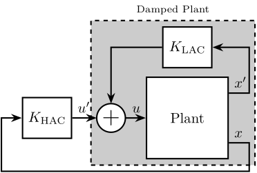
- HAC-LAC (Figure ref:fig:detail_control_architecture_hac_lac) cite:&geng95_intel_contr_system_multip_degree;&preumont18_vibrat_contr_activ_struc_fourt_edition;&wang16_inves_activ_vibrat_isolat_stewar;&li01_simul_vibrat_isolat_point_contr;&pu11_six_degree_of_freed_activ;&xie17_model_contr_hybrid_passiv_activ
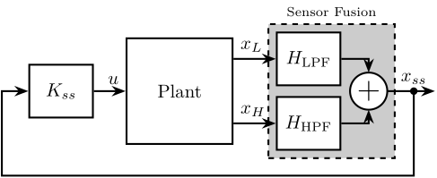
- Sensor Fusion (Figure ref:fig:detail_control_architecture_sensor_fusion) cite:&tjepkema12_activ_ph;&tjepkema12_sensor_fusion_activ_vibrat_isolat_precis_equip;&hauge04_sensor_contr_space_based_six
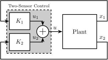
- Two Sensor control (Figure ref:fig:detail_control_architecture_two_sensor_control) cite:&hauge04_sensor_contr_space_based_six;&tjepkema12_activ_ph;&beijen14_two_sensor_contr_activ_vibrat;&yong16_high_speed_vertic_posit_stage
-
Explain basic idea for three strategies:
- HAC-LAC: sequential control.
- Sensor Fusion: use different sensors in different frequency regions for different reasons: noise, robustness, …
- Two sensor control: idea is to have the maximum control on how both sensors are utilized. Theoretically, this could give the best performances (as sensor fusion is a special case of two sensor control). But it may be more complex to tune and analyze.
Comparison between "two sensor control" and "sensor fusion" is given in cite:&beijen14_two_sensor_contr_activ_vibrat.
\begin{tikzpicture}
  % Blocs
  \node[block={2.0cm}{2.0cm}] (P) {Plant};
  \coordinate[] (input)   at ($(P.south west)!0.5!(P.north west)$);
  \coordinate[] (outputH) at ($(P.south east)!0.2!(P.north east)$);
  \coordinate[] (outputL) at ($(P.south east)!0.8!(P.north east)$);

  \node[block, above=0.2 of P] (Klac) {$K_\text{LAC}$};
  \node[addb, left=0.5 of input] (addF) {};
  \node[block, left=0.6 of addF] (Khac) {$K_\text{HAC}$};
  % \node[addb={+}{}{}{}{-}, left=0.5 of Khac] (subr) {};

  % Connections and labels
  \draw[->] (outputL) -- ++(0.5, 0) coordinate(eastlac) |- (Klac.east);
  \node[above right] at (outputL){$x^\prime$};
  \draw[->] (Klac.west) -| (addF.north);
  \draw[->] (addF.east) -- (input) node[above left]{$u$};

  % \draw[<-] (subr.west)node[above left]{$r$} -- ++(-0.5, 0);
  % \draw[->] (outputH) -- ++(0.5, 0)  -- ++(0, -1.0) -| (subr.south);
  \draw[->] (outputH) -- ++(0.5, 0)  -- ++(0, -0.7) -| ($(Khac.west)+(-0.5, 0)$) -- (Khac.west);
  \node[above right] at (outputH){$x$};
  % \draw[->] (subr.east) -- (Khac.west) node[above left]{$\epsilon$};
  \draw[->] (Khac.east) node[above right]{$u^\prime$} -- (addF.west);

  \begin{scope}[on background layer]
    \node[fit={(Klac.north-|eastlac) (addF.west|-P.south)}, fill=black!20!white, draw, dashed, inner sep=4pt] (Pi) {};
    % \node[anchor={north west}, align=left] at (Pi.north west){\scriptsize{Damped}\\\scriptsize{Plant}};
    \node[above=0 of Pi]{\scriptsize{Damped Plant}};
  \end{scope}
\end{tikzpicture}\begin{tikzpicture}
% Blocs
\node[block={2.0cm}{2.0cm}] (P) {Plant};
\coordinate[] (input) at ($(P.south west)!0.5!(P.north west)$);
\coordinate[] (outputH) at ($(P.south east)!0.2!(P.north east)$);
\coordinate[] (outputL) at ($(P.south east)!0.8!(P.north east)$);
\coordinate[] (outputSS) at ($(P.south east)!0.5!(P.north east)$);
\node[block, right=0.8 of outputH] (KH) {$H_\text{HPF}$};
\node[block, right=0.8 of outputL] (KL) {$H_\text{LPF}$};
\node[addb={+}{}{}{}{}, right=2.2 of outputSS] (addss) {};
\node[block, left=0.6 of input] (K) {$K_{ss}$};
% Connections and labels
\draw[->] (outputL) -- (KL.west);
\draw[->] (outputH) -- (KH.west);
\node[above right] at (outputL){$x_L$};
\node[above right] at (outputH){$x_H$};
\draw[->] (KL.east) -| (addss.north);
\draw[->] (KH.east) -| (addss.south);
\draw[->] (addss.east) -- ++(0.9, 0);
\draw[->] ($(addss.east) + (0.5, 0)$)node[branch]{}node[above]{$x_{ss}$} -- ++(0, -1.6) -| ($(K.west)+(-0.5, 0)$) -- (K.west);
\draw[->] (K.east) -- (input) node[above left]{$u$};
\begin{scope}[on background layer]
\node[fit={(KL.north west) (KH.south-|addss.east)}, fill=black!20!white, draw, dashed, inner sep=4pt] (Pss) {};
\node[above=0 of Pss]{\scriptsize{Sensor Fusion}};
\end{scope}
\end{tikzpicture}\begin{tikzpicture}
% Blocs
\node[block={2.0cm}{2.0cm}] (P) {Plant};
\coordinate[] (input) at ($(P.south west)!0.5!(P.north west)$);
\coordinate[] (output1) at ($(P.south east)!0.8!(P.north east)$);
\coordinate[] (output2) at ($(P.south east)!0.2!(P.north east)$);
\node[addb={+}{}{}{}{}, left=0.8 of input] (addF) {};
\coordinate[left= 1.0 of addF] (Ks);
\node[block] (K1) at (Ks|-output1) {$K_\text{1}$};
\node[block] (K2) at (Ks|-output2) {$K_\text{2}$};
\draw[->] (output1) -| ++(0.6, 1.2) -| ($(K1.west)+(-0.5, 0)$) -- (K1.west);
\draw[->] (output2) -| ++(0.6,-1.0) -| ($(K2.west)+(-0.5, 0)$) -- (K2.west);
\draw[->] (K1.east)node[above right]{$u_1$} -| (addF.north);
\draw[->] (K2.east)node[above right]{$u_2$} -| (addF.south);
\draw[->] (addF.east) -- (input) node[above left=0 and 0.2]{$u$};
\node[above right] at (output1){$x_1$};
\node[above right] at (output2){$x_2$};
\begin{scope}[on background layer]
\node[fit={(K1.north west) (K2.south-|addF.east)}, fill=black!20!white, draw, dashed, inner sep=4pt] (Pss) {};
\node[above=0 of Pss]{\scriptsize{Two-Sensor Control}};
\end{scope}
\end{tikzpicture}The use of multiple sensors have already been used for the Stewart platform. Table ref:tab:detail_control_multiple_sensor_review
| Actuators | Sensors | Control | Main Object | Reference |
|---|---|---|---|---|
| Magnetostrictive | Force (collocated), Accelerometers | Two layers: Decentralized IFF, Robust Adaptive Control | Two layer control for active damping and vibration isolation | cite:&geng95_intel_contr_system_multip_degree |
| Piezoelectric | Force Sensor + Accelerometer | HAC-LAC (IFF + FxLMS) | Dynamic Model + Vibration Control | cite:&wang16_inves_activ_vibrat_isolat_stewar |
| Voice Coil | Accelerometer (collocated), ext. Rx/Ry sensors | Cartesian acceleration feedback (isolation) + 2DoF pointing control (external sensor) | Decoupling, both vibration + pointing control | cite:&li01_simul_vibrat_isolat_point_contr |
| Voice Coil | Geophone + Eddy Current (Struts, collocated) | Decentralized (Sky Hook) + Centralized (modal) Control | cite:&pu11_six_degree_of_freed_activ | |
| Voice Coil | Force sensors (strus) + accelerometer (cartesian) | Decentralized Force Feedback + Centralized H2 control based on accelerometers | cite:&xie17_model_contr_hybrid_passiv_activ | |
| Voice Coil | Force (HF) and Inertial (LF) | Sensor Fusion, Two Sensor Control | cite:&tjepkema12_activ_ph;&tjepkema12_sensor_fusion_activ_vibrat_isolat_precis_equip | |
| Voice Coil | Force (HF) and Inertial (LF) | Sensor Fusion, LQG, Decentralized | Combine force/inertial sensors. Comparison of force sensor and inertial sensors. Issue on non-minimum phase zero | cite:&hauge04_sensor_contr_space_based_six |
| Piezoelectric | Force, Position | Vibration isolation, Model-Based, Modal control: 6x PI controllers | Stiffness of flexible joints is compensated using feedback, then the system is decoupled in the modal space | cite:&yang19_dynam_model_decoup_contr_flexib |
| Voice Coil | Force, LVDT, Geophones | LQG, Force + geophones for vibration, LVDT for pointing | Centralized control is no better than decentralized. Geophone + Force MISO control is good | cite:&thayer98_stewar;&thayer02_six_axis_vibrat_isolat_system |
| Voice Coil | Force | IFF, centralized (decouple) + decentralized (coupled) | Specific geometry: decoupled force plant. Better perf with centralized IFF | cite:&mcinroy99_dynam;&mcinroy99_precis_fault_toler_point_using_stewar_platf;&mcinroy00_desig_contr_flexur_joint_hexap |
Cascaded control / HAC-LAC Architecture was already discussed during the conceptual phase. This is a very comprehensive approach that proved to give good performances.
On the other hand of the spectrum, the two sensor approach yields to more control design freedom. But it is also more complex.
In this section, we wish to study if sensor fusion can be an option for multi-sensor control:
- may be used to optimize the noise characteristics
- optimize the dynamical uncertainty
Sensor fusion - Introduction
Measuring a physical quantity using sensors is always subject to several limitations. First, the accuracy of the measurement is affected by several noise sources, such as electrical noise of the conditioning electronics being used. Second, the frequency range in which the measurement is relevant is bounded by the bandwidth of the sensor. One way to overcome these limitations is to combine several sensors using a technique called "sensor fusion" cite:&bendat57_optim_filter_indep_measur_two. Fortunately, a wide variety of sensors exists, each with different characteristics. By carefully choosing the fused sensors, a so called "super sensor" is obtained that can combines benefits of the individual sensors.
In some situations, sensor fusion is used to increase the bandwidth of the measurement cite:&shaw90_bandw_enhan_posit_measur_using_measur_accel;&zimmermann92_high_bandw_orien_measur_contr;&min15_compl_filter_desig_angle_estim. For instance, in cite:&shaw90_bandw_enhan_posit_measur_using_measur_accel the bandwidth of a position sensor is increased by fusing it with an accelerometer providing the high frequency motion information. For other applications, sensor fusion is used to obtain an estimate of the measured quantity with lower noise cite:&hua05_low_ligo;&hua04_polyp_fir_compl_filter_contr_system;&plummer06_optim_compl_filter_their_applic_motion_measur;&robert12_introd_random_signal_applied_kalman. More recently, the fusion of sensors measuring different physical quantities has been proposed to obtain interesting properties for control cite:&collette15_sensor_fusion_method_high_perfor;&yong16_high_speed_vertic_posit_stage. In cite:&collette15_sensor_fusion_method_high_perfor, an inertial sensor used for active vibration isolation is fused with a sensor collocated with the actuator for improving the stability margins of the feedback controller.
Practical applications of sensor fusion are numerous. It is widely used for the attitude estimation of several autonomous vehicles such as unmanned aerial vehicle cite:&baerveldt97_low_cost_low_weigh_attit;&corke04_inert_visual_sensin_system_small_auton_helic;&jensen13_basic_uas and underwater vehicles cite:&pascoal99_navig_system_desig_using_time;&batista10_optim_posit_veloc_navig_filter_auton_vehic. Naturally, it is of great benefits for high performance positioning control as shown in cite:&shaw90_bandw_enhan_posit_measur_using_measur_accel;&zimmermann92_high_bandw_orien_measur_contr;&min15_compl_filter_desig_angle_estim;&yong16_high_speed_vertic_posit_stage. Sensor fusion was also shown to be a key technology to improve the performance of active vibration isolation systems cite:&tjepkema12_sensor_fusion_activ_vibrat_isolat_precis_equip. Emblematic examples are the isolation stages of gravitational wave detectors cite:&collette15_sensor_fusion_method_high_perfor;&heijningen18_low such as the ones used at the LIGO cite:&hua05_low_ligo;&hua04_polyp_fir_compl_filter_contr_system and at the Virgo cite:&lucia18_low_frequen_optim_perfor_advan.
There are mainly two ways to perform sensor fusion: either using a set of complementary filters cite:&anderson53_instr_approac_system_steer_comput or using Kalman filtering cite:&brown72_integ_navig_system_kalman_filter. For sensor fusion applications, both methods are sharing many relationships cite:&brown72_integ_navig_system_kalman_filter;&higgins75_compar_compl_kalman_filter;&robert12_introd_random_signal_applied_kalman;&fonseca15_compl. However, for Kalman filtering, assumptions must be made about the probabilistic character of the sensor noises cite:&robert12_introd_random_signal_applied_kalman whereas it is not the case with complementary filters. Furthermore, the advantages of complementary filters over Kalman filtering for sensor fusion are their general applicability, their low computational cost cite:&higgins75_compar_compl_kalman_filter, and the fact that they are intuitive as their effects can be easily interpreted in the frequency domain.
A set of filters is said to be complementary if the sum of their transfer functions is equal to one at all frequencies. In the early days of complementary filtering, analog circuits were employed to physically realize the filters cite:&anderson53_instr_approac_system_steer_comput. Analog complementary filters are still used today cite:&yong16_high_speed_vertic_posit_stage;&moore19_capac_instr_sensor_fusion_high_bandw_nanop, but most of the time they are now implemented digitally as it allows for much more flexibility.
Several design methods have been developed over the years to optimize complementary filters. The easiest way to design complementary filters is to use analytical formulas. Depending on the application, the formulas used are of first order cite:&corke04_inert_visual_sensin_system_small_auton_helic;&yeh05_model_contr_hydraul_actuat_two;&yong16_high_speed_vertic_posit_stage, second order cite:&baerveldt97_low_cost_low_weigh_attit;&stoten01_fusion_kinet_data_using_compos_filter;&jensen13_basic_uas or even higher orders cite:&shaw90_bandw_enhan_posit_measur_using_measur_accel;&zimmermann92_high_bandw_orien_measur_contr;&stoten01_fusion_kinet_data_using_compos_filter;&collette15_sensor_fusion_method_high_perfor;&matichard15_seism_isolat_advan_ligo.
As the characteristics of the super sensor depends on the proper design of the complementary filters cite:&dehaeze19_compl_filter_shapin_using_synth, several optimization techniques have been developed. Some are based on the finding of optimal parameters of analytical formulas cite:&jensen13_basic_uas;&min15_compl_filter_desig_angle_estim;&fonseca15_compl, while other are using convex optimization tools cite:&hua04_polyp_fir_compl_filter_contr_system;&hua05_low_ligo such as linear matrix inequalities cite:&pascoal99_navig_system_desig_using_time. As shown in cite:&plummer06_optim_compl_filter_their_applic_motion_measur, the design of complementary filters can also be linked to the standard mixed-sensitivity control problem. Therefore, all the powerful tools developed for the classical control theory can also be used for the design of complementary filters. For instance, in cite:&jensen13_basic_uas the two gains of a Proportional Integral (PI) controller are optimized to minimize the noise of the super sensor.
The common objective of all these complementary filters design methods is to obtain a super sensor that has desired characteristics, usually in terms of noise and dynamics. Moreover, as reported in cite:&zimmermann92_high_bandw_orien_measur_contr;&plummer06_optim_compl_filter_their_applic_motion_measur, phase shifts and magnitude bumps of the super sensors dynamics can be observed if either the complementary filters are poorly designed or if the sensors are not well calibrated. Hence, the robustness of the fusion is also of concern when designing the complementary filters. Although many design methods of complementary filters have been proposed in the literature, no simple method that allows to specify the desired super sensor characteristic while ensuring good fusion robustness has been proposed.
Fortunately, both the robustness of the fusion and the super sensor characteristics can be linked to the magnitude of the complementary filters cite:&dehaeze19_compl_filter_shapin_using_synth. Based on that, this work introduces a new way to design complementary filters using the $\mathcal{H}_\infty$ synthesis which allows to shape the complementary filters' magnitude in an easy and intuitive way.
Sensor Fusion and Complementary Filters Requirements
<<ssec:detail_control_sensor_fusion_requirements>>
Introduction ignore
Complementary filtering provides a framework for fusing signals from different sensors. As the effectiveness of the fusion depends on the proper design of the complementary filters, they are expected to fulfill certain requirements. These requirements are discussed in this section.
Sensor Fusion Architecture
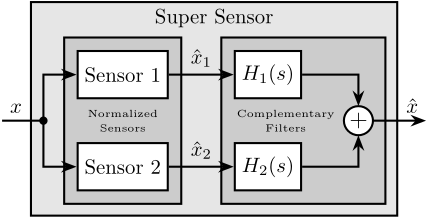
A general sensor fusion architecture using complementary filters is shown in Figure ref:fig:detail_control_sensor_fusion_overview where several sensors (here two) are measuring the same physical quantity $x$. The two sensors output signals $\hat{x}_1$ and $\hat{x}_2$ are estimates of $x$. These estimates are then filtered out by complementary filters and combined to form a new estimate $\hat{x}$.
The resulting sensor, termed as "super sensor", can have larger bandwidth and better noise characteristics in comparison to the individual sensors. This means that the super sensor provides an estimate $\hat{x}$ of $x$ which can be more accurate over a larger frequency band than the outputs of the individual sensors.
\tikzset{block/.default={0.8cm}{0.8cm}}
\tikzset{addb/.append style={scale=0.7}}
\tikzset{node distance=0.6}
\begin{tikzpicture}
  \node[branch] (x) at (0, 0);
  \node[block, above right=0.3 and 0.5 of x](sensor1){Sensor 1};
  \node[block, below right=0.3 and 0.5 of x](sensor2){Sensor 2};

  \node[block, right=1.1 of sensor1](H1){$H_1(s)$};
  \node[block, right=1.1 of sensor2](H2){$H_2(s)$};

  \node[addb, right=5.0 of x](add){};

  \draw[] ($(x)+(-0.7, 0)$) node[above right]{$x$} -- (x.center);
  \draw[->] (x.center) |- (sensor1.west);
  \draw[->] (x.center) |- (sensor2.west);
  \draw[->] (sensor1.east) -- node[midway, above]{$\hat{x}_1$} (H1.west);
  \draw[->] (sensor2.east) -- node[midway, above]{$\hat{x}_2$} (H2.west);
  \draw[->] (H1) -| (add.north);
  \draw[->] (H2) -| (add.south);
  \draw[->] (add.east) -- ++(0.9, 0) node[above left]{$\hat{x}$};

  \begin{scope}[on background layer]
    \node[fit={($(H2.south-|x) + (0, -0.2)$) ($(H1.north-|add.east) + (0.2, 0.6)$)}, fill=black!10!white, draw, inner sep=6pt] (supersensor) {};
    \node[below] at (supersensor.north) {Super Sensor};

    \node[fit={(sensor2.south west) (sensor1.north east)}, fill=black!20!white, draw, inner sep=6pt] (sensors) {};
    \node[align=center] at (sensors.center) {{\tiny Normalized}\\[-0.5em]{\tiny Sensors}};

    \node[fit={(H2.south west) (H1.north-|add.east)}, fill=black!20!white, draw, inner sep=6pt] (filters) {};
    \node[align=center] at ($(filters.center) + (-0.3, 0)$) {{\tiny Complementary}\\[-0.5em]{\tiny Filters}};
  \end{scope}
\end{tikzpicture}The complementary property of filters $H_1(s)$ and $H_2(s)$ implies that the sum of their transfer functions is equal to one eqref:eq:detail_control_comp_filter. That is, unity magnitude and zero phase at all frequencies.
\begin{equation}\label{eq:detail_control_comp_filter} H_1(s) + H_2(s) = 1
\end{equation}
Sensor Models and Sensor Normalization
In order to study such sensor fusion architecture, a model for the sensors is required. Such model is shown in Figure ref:fig:detail_control_sensor_model and consists of a linear time invariant (LTI) system $G_i(s)$ representing the sensor dynamics and an input $n_i$ representing the sensor noise. The model input $x$ is the measured physical quantity and its output $\tilde{x}_i$ is the "raw" output of the sensor.
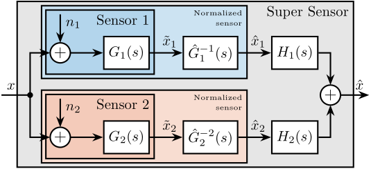
Before filtering the sensor outputs $\tilde{x}_i$ by the complementary filters, the sensors are usually normalized to simplify the fusion. This normalization consists of using an estimate $\hat{G}_i(s)$ of the sensor dynamics $G_i(s)$, and filtering the sensor output by the inverse of this estimate $\hat{G}_i^{-1}(s)$ as shown in Figure ref:fig:detail_control_sensor_model_calibrated. It is here supposed that the sensor inverse $\hat{G}_i^{-1}(s)$ is proper and stable. This way, the units of the estimates $\hat{x}_i$ are equal to the units of the physical quantity $x$. The sensor dynamics estimate $\hat{G}_i(s)$ can be a simple gain or a more complex transfer function.
\tikzset{block/.default={0.8cm}{0.8cm}}
\tikzset{addb/.append style={scale=0.7}}
\tikzset{node distance=0.6}
\begin{tikzpicture}
  \node[addb](add1){};
  \node[block, right=0.8 of add1](G1){$G_i(s)$};

  \draw[->] ($(add1.west)+(-0.7, 0)$) node[above right]{$x$} -- (add1.west);
  \draw[<-] (add1.north) -- ++(0, 0.7)node[below right](n1){$n_i$};
  \draw[->] (add1.east) -- (G1.west);
  \draw[->] (G1.east) -- ++(0.7, 0) node[above left]{$\tilde{x}_i$};

  \begin{scope}[on background layer]
    \node[fit={(add1.west |- G1.south) (n1.north -| G1.east)}, fill=black!20!white, draw, inner sep=3pt] (sensor1) {};
    \node[below left] at (sensor1.north east) {Sensor};
  \end{scope}
\end{tikzpicture}\tikzset{block/.default={0.8cm}{0.8cm}}
\tikzset{addb/.append style={scale=0.7}}
\tikzset{node distance=0.6}
\begin{tikzpicture}
\node[addb](add1){};
\node[block, right=0.8 of add1](G1){$G_i(s)$};
\node[block, right=0.8 of G1](G1inv){$\hat{G}_i^{-1}(s)$};
\draw[->] ($(add1.west)+(-0.7, 0)$) node[above right]{$x$} -- (add1.west);
\draw[<-] (add1.north) -- ++(0, 0.7)node[below right](n1){$n_i$};
\draw[->] (add1.east) -- (G1.west);
\draw[->] (G1.east) -- (G1inv.west) node[above left]{$\tilde{x}_i$};
\draw[->] (G1inv.east) -- ++(0.8, 0) node[above left]{$\hat{x}_i$};
\begin{scope}[on background layer]
\node[fit={(add1.west |- G1inv.south) (n1.north -| G1inv.east)}, fill=black!10!white, draw, inner sep=6pt] (sensor1cal) {};
\node[below left, align=right] at (sensor1cal.north east) {{\tiny Normalized}\\[-0.5em]{\tiny sensor}};
\node[fit={(add1.west |- G1.south) (n1.north -| G1.east)}, fill=black!20!white, draw, inner sep=3pt] (sensor1) {};
\node[below left] at (sensor1.north east) {Sensor};
\end{scope}
\end{tikzpicture}Two normalized sensors are then combined to form a super sensor as shown in Figure ref:fig:detail_control_fusion_super_sensor. The two sensors are measuring the same physical quantity $x$ with dynamics $G_1(s)$ and $G_2(s)$, and with uncorrelated noises $n_1$ and $n_2$. The signals from both normalized sensors are fed into two complementary filters $H_1(s)$ and $H_2(s)$ and then combined to yield an estimate $\hat{x}$ of $x$. The super sensor output $\hat{x}$ is therefore described by eqref:eq:detail_control_comp_filter_estimate.
\begin{equation}\label{eq:detail_control_comp_filter_estimate} \hat{x} = \Big( H_1(s) \hat{G}_1-1(s) G_1(s) + H_2(s) \hat{G}_2-1(s) G_2(s) \Big) x + H_1(s) \hat{G}_1-1(s) G_1(s) n_1 + H_2(s) \hat{G}_2-1(s) G_2(s) n_2
\end{equation}
\tikzset{block/.default={0.8cm}{0.8cm}}
\tikzset{addb/.append style={scale=0.7}}
\tikzset{node distance=0.6}
\begin{tikzpicture}
  \node[branch] (x) at (0, 0);
  \node[addb, above right=0.8 and 0.5 of x](add1){};
  \node[addb, below right=0.8 and 0.5 of x](add2){};
  \node[block, right=0.8 of add1](G1){$G_1(s)$};
  \node[block, right=0.8 of add2](G2){$G_2(s)$};
  \node[block, right=0.8 of G1](G1inv){$\hat{G}_1^{-1}(s)$};
  \node[block, right=0.8 of G2](G2inv){$\hat{G}_2^{-2}(s)$};
  \node[block, right=0.8 of G1inv](H1){$H_1(s)$};
  \node[block, right=0.8 of G2inv](H2){$H_2(s)$};
  \node[addb, right=7 of x](add){};

  \draw[] ($(x)+(-0.7, 0)$) node[above right]{$x$} -- (x.center);
  \draw[->] (x.center) |- (add1.west);
  \draw[->] (x.center) |- (add2.west);
  \draw[<-] (add1.north) -- ++(0, 0.7)node[below right](n1){$n_1$};
  \draw[->] (add1.east) -- (G1.west);
  \draw[->] (G1.east) -- (G1inv.west) node[above left]{$\tilde{x}_1$};
  \draw[->] (G1inv.east) -- (H1.west) node[above left]{$\hat{x}_1$};
  \draw[<-] (add2.north) -- ++(0, 0.7)node[below right](n2){$n_2$};
  \draw[->] (add2.east) -- (G2.west);
  \draw[->] (G2.east) -- (G2inv.west) node[above left]{$\tilde{x}_2$};
  \draw[->] (G2inv.east) -- (H2.west) node[above left]{$\hat{x}_2$};
  \draw[->] (H1) -| (add.north);
  \draw[->] (H2) -| (add.south);
  \draw[->] (add.east) -- ++(0.7, 0) node[above left]{$\hat{x}$};

  \begin{scope}[on background layer]
    \node[fit={(G2.south-|x) (n1.north-|add.east)}, fill=black!10!white, draw, inner sep=9pt] (supersensor) {};
    \node[below left] at (supersensor.north east) {Super Sensor};

    \node[fit={(add1.west |- G1inv.south) (n1.north -| G1inv.east)}, fill=colorblue!20!white, draw, inner sep=6pt] (sensor1cal) {};
    \node[below left, align=right] at (sensor1cal.north east) {{\tiny Normalized}\\[-0.5em]{\tiny sensor}};
    \node[fit={(add1.west |- G1.south) (n1.north -| G1.east)}, fill=colorblue!30!white, draw, inner sep=3pt] (sensor1) {};
    \node[below left] at (sensor1.north east) {Sensor 1};

    \node[fit={(add2.west |- G2inv.south) (n2.north -| G2inv.east)}, fill=colorred!20!white, draw, inner sep=6pt] (sensor2cal) {};
    \node[below left, align=right] at (sensor2cal.north east) {{\tiny Normalized}\\[-0.5em]{\tiny sensor}};
    \node[fit={(add2.west |- G2.south) (n2.north -| G2.east)}, fill=colorred!30!white, draw, inner sep=3pt] (sensor2) {};
    \node[below left] at (sensor2.north east) {Sensor 2};
  \end{scope}
\end{tikzpicture}Noise Sensor Filtering
First, suppose that all the sensors are perfectly normalized eqref:eq:detail_control_perfect_dynamics. The effect of a non-perfect normalization will be discussed afterwards.
\begin{equation}\label{eq:detail_control_perfect_dynamics} \frac{\hat{x}_i}{x} = \hat{G}_i(s) G_i(s) = 1
\end{equation}
Provided eqref:eq:detail_control_perfect_dynamics is verified, the super sensor output $\hat{x}$ is then equal to $x$ plus the filtered noise of both sensors eqref:eq:detail_control_estimate_perfect_dyn. From eqref:eq:detail_control_estimate_perfect_dyn, the complementary filters $H_1(s)$ and $H_2(s)$ are shown to only operate on the noise of the sensors. Thus, this sensor fusion architecture permits to filter the noise of both sensors without introducing any distortion in the physical quantity to be measured. This is why the two filters must be complementary.
\begin{equation}\label{eq:detail_control_estimate_perfect_dyn} \hat{x} = x + H_1(s) n_1 + H_2(s) n_2
\end{equation}
The estimation error $\delta x$, defined as the difference between the sensor output $\hat{x}$ and the measured quantity $x$, is computed for the super sensor eqref:eq:detail_control_estimate_error.
\begin{equation}\label{eq:detail_control_estimate_error} δ x ≜ \hat{x} - x = H_1(s) n_1 + H_2(s) n_2
\end{equation}
As shown in eqref:eq:detail_control_noise_filtering_psd, the Power Spectral Density (PSD) of the estimation error $\Phi_{\delta x}$ depends both on the norm of the two complementary filters and on the PSD of the noise sources $\Phi_{n_1}$ and $\Phi_{n_2}$.
\begin{equation}\label{eq:detail_control_noise_filtering_psd} Φδ x(ω) = ≤ft|H_1(jω)\right|^2 Φn_1(ω) + ≤ft|H_2(jω)\right|^2 Φn_2(ω)
\end{equation}
If the two sensors have identical noise characteristics, $\Phi_{n_1}(\omega) = \Phi_{n_2}(\omega)$, a simple averaging ($H_1(s) = H_2(s) = 0.5$) is what would minimize the super sensor noise. This is the simplest form of sensor fusion with complementary filters.
However, the two sensors have usually high noise levels over distinct frequency regions. In such case, to lower the noise of the super sensor, the norm $|H_1(j\omega)|$ has to be small when $\Phi_{n_1}(\omega)$ is larger than $\Phi_{n_2}(\omega)$ and the norm $|H_2(j\omega)|$ has to be small when $\Phi_{n_2}(\omega)$ is larger than $\Phi_{n_1}(\omega)$. Hence, by properly shaping the norm of the complementary filters, it is possible to minimize the noise of the super sensor.
Sensor Fusion Robustness
In practical systems the sensor normalization is not perfect and condition eqref:eq:detail_control_perfect_dynamics is not verified.
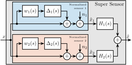
In order to study such imperfection, a multiplicative input uncertainty is added to the sensor dynamics (Figure ref:fig:detail_control_sensor_model_uncertainty). The nominal model is the estimated model used for the normalization $\hat{G}_i(s)$, $\Delta_i(s)$ is any stable transfer function satisfying $|\Delta_i(j\omega)| \le 1,\ \forall\omega$, and $w_i(s)$ is a weighting transfer function representing the magnitude of the uncertainty. The weight $w_i(s)$ is chosen such that the real sensor dynamics $G_i(j\omega)$ is contained in the uncertain region represented by a circle in the complex plane, centered on $1$ and with a radius equal to $|w_i(j\omega)|$.
As the nominal sensor dynamics is taken as the normalized filter, the normalized sensor can be further simplified as shown in Figure ref:fig:detail_control_sensor_model_uncertainty_simplified.
\tikzset{block/.default={0.8cm}{0.8cm}}
\tikzset{addb/.append style={scale=0.7}}
\tikzset{node distance=0.6}
\begin{tikzpicture}
  \node[branch] (input) at (0,0) {};
  \node[block, above right= 0.4 and 0.4 of input](W1){$w_1(s)$};
  \node[block, right=0.4 of W1](delta1){$\Delta_1(s)$};
  \node[addb] (addu) at ($(delta1.east|-input) + (0.4, 0)$) {};
  \node[addb, right=0.4 of addu] (addn) {};
  \node[block, right=0.4 of addn] (G1) {$\hat{G}_1(s)$};
  \node[block, right=0.8 of G1](G1inv){$\hat{G}_1^{-1}(s)$};

  \draw[->] ($(input)+(-0.7, 0)$) node[above right]{$x$} -- (addu);
  \draw[->] (input.center) |- (W1.west);
  \draw[->] (W1.east) -- (delta1.west);
  \draw[->] (delta1.east) -| (addu.north);
  \draw[->] (addu.east) -- (addn.west);
  \draw[->] (addn.east) -- (G1.west);
  \draw[<-] (addn.north) -- ++(0, 0.7)node[below right](n1){$n_1$};
  \draw[->] (G1.east) -- (G1inv.west) node[above left]{$\tilde{x}_1$};
  \draw[->] (G1inv.east) -- ++(0.8, 0) node[above left]{$\hat{x}_1$};

  \begin{scope}[on background layer]
    \node[fit={(input.west |- G1inv.south) (delta1.north -| G1inv.east)}, fill=black!10!white, draw, inner sep=6pt] (sensor1cal) {};
    \node[below left, align=right] at (sensor1cal.north east) {{\tiny Normalized}\\[-0.5em]{\tiny sensor}};

    \node[fit={(input.west |- G1.south) (delta1.north -| G1.east)}, fill=black!20!white, draw, inner sep=3pt] (sensor1) {};
    \node[below left] at (sensor1.north east) {Sensor};
  \end{scope}
\end{tikzpicture}\tikzset{block/.default={0.8cm}{0.8cm}}
\tikzset{addb/.append style={scale=0.7}}
\tikzset{node distance=0.6}
\begin{tikzpicture}
\node[branch] (input) at (0,0) {};
\node[block, above right= 0.4 and 0.4 of input](W1){$w_1(s)$};
\node[block, right=0.4 of W1](delta1){$\Delta_1(s)$};
\node[addb] (addu) at ($(delta1.east|-input) + (0.4, 0)$) {};
\node[addb, right=0.4 of addu] (addn) {};
\draw[->] ($(input)+(-0.8, 0)$) node[above right]{$x$} -- (addu);
\draw[->] (input.center) |- (W1.west);
\draw[->] (W1.east) -- (delta1.west);
\draw[->] (delta1.east) -| (addu.north);
\draw[->] (addu.east) -- (addn.west);
\draw[<-] (addn.north) -- ++(0, 0.6)node[below right](n1){$n_1$};
\draw[->] (addn.east) -- ++(0.9, 0) node[above left]{$\hat{x}_1$};
\begin{scope}[on background layer]
\node[fit={(input.west |- addu.south) ($(delta1.north -| addn.east) + (0.1, 0)$)}, fill=black!10!white, draw, inner sep=6pt] (sensor1cal) {};
\node[below left, align=right] at (sensor1cal.north east) {{\tiny Normalized}\\[-0.5em]{\tiny sensor}};
\end{scope}
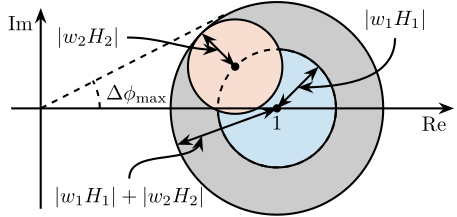
\end{tikzpicture}The sensor fusion architecture with the sensor models including dynamical uncertainty is shown in Figure ref:fig:detail_control_sensor_fusion_dynamic_uncertainty. The super sensor dynamics eqref:eq:detail_control_super_sensor_dyn_uncertainty is no longer equal to $1$ and now depends on the sensor dynamical uncertainty weights $w_i(s)$ as well as on the complementary filters $H_i(s)$. The dynamical uncertainty of the super sensor can be graphically represented in the complex plane by a circle centered on $1$ with a radius equal to $|w_1(j\omega) H_1(j\omega)| + |w_2(j\omega) H_2(j\omega)|$ (Figure ref:fig:detail_control_uncertainty_set_super_sensor).
\begin{equation}\label{eq:detail_control_super_sensor_dyn_uncertainty} \frac{\hat{x}}{x} = 1 + w_1(s) H_1(s) Δ_1(s) + w_2(s) H_2(s) Δ_2(s)
\end{equation}
\tikzset{block/.default={0.8cm}{0.8cm}}
\tikzset{addb/.append style={scale=0.7}}
\tikzset{node distance=0.6}
\begin{tikzpicture}
  \node[branch] (x) at (0, 0);

  \node[branch, above right=1.0 and 0.3 of x] (input1) {};
  \node[branch, below right=1.0 and 0.3 of x] (input2) {};
  \node[block, above right= 0.4 and 0.3 of input1](W1){$w_1(s)$};
  \node[block, above right= 0.4 and 0.3 of input2](W2){$w_2(s)$};
  \node[block, right=0.4 of W1](delta1){$\Delta_1(s)$};
  \node[block, right=0.4 of W2](delta2){$\Delta_2(s)$};
  \node[addb] (addu1) at ($(delta1.east|-input1) + (0.4, 0)$) {};
  \node[addb] (addu2) at ($(delta2.east|-input2) + (0.4, 0)$) {};
  \node[addb, right=0.4 of addu1] (addn1) {};
  \node[addb, right=0.4 of addu2] (addn2) {};
  \node[block, right=0.9 of addn1](H1){$H_1(s)$};
  \node[block, right=0.9 of addn2](H2){$H_2(s)$};

  \node[addb, right=7 of x](add){};


  \draw[] ($(x)+(-0.7, 0)$) node[above right]{$x$} -- (x.center);
  \draw[->] (x.center) |- (addu1.west);
  \draw[->] (x.center) |- (addu2.west);
  \draw[->] (input1.center) |- (W1.west);
  \draw[->] (W1.east) -- (delta1.west);
  \draw[->] (delta1.east) -| (addu1.north);
  \draw[->] (addu1.east) -- (addn1.west);
  \draw[<-] (addn1.north) -- ++(0, 0.6)node[below right](n1){$n_1$};
  \draw[->] (input2.center) |- (W2.west);
  \draw[->] (W2.east) -- (delta2.west);
  \draw[->] (delta2.east) -| (addu2.north);
  \draw[->] (addu2.east) -- (addn2.west);
  \draw[<-] (addn2.north) -- ++(0, 0.6)node[below right](n2){$n_2$};

  \draw[->] (addn1.east) -- (H1.west) node[above left]{$\hat{x}_1$};
  \draw[->] (addn2.east) -- (H2.west) node[above left]{$\hat{x}_2$};
  \draw[->] (H1) -| (add.north);
  \draw[->] (H2) -| (add.south);
  \draw[->] (add.east) -- ++(0.7, 0) node[above left]{$\hat{x}$};

  \begin{scope}[on background layer]
    \node[fit={(addn2.south-|x) (delta1.north-|add.east)}, fill=black!10!white, draw, inner sep=9pt] (supersensor) {};
    \node[below left] at (supersensor.north east) {Super Sensor};

    \node[fit={(input1.west |- addu1.south) ($(delta1.north -| addn1.east) + (0.1, 0.0)$)}, fill=colorblue!20!white, draw, inner sep=6pt] (sensor1cal) {};
    \node[below left, align=right] at (sensor1cal.north east) {{\tiny Normalized}\\[-0.5em]{\tiny sensor 1}};

    \node[fit={(input2.west |- addu2.south) ($(delta2.north -| addn1.east) + (0.1, 0.0)$)}, fill=colorred!20!white, draw, inner sep=6pt] (sensor2cal) {};
    \node[below left, align=right] at (sensor2cal.north east) {{\tiny Normalized}\\[-0.5em]{\tiny sensor 2}};
  \end{scope}
\end{tikzpicture}\tikzset{block/.default={0.8cm}{0.8cm}}
\tikzset{addb/.append style={scale=0.7}}
\tikzset{node distance=0.6}
\begin{tikzpicture}
\begin{scope}[shift={(4, 0)}]
% Uncertainty Circle
\node[draw, circle, fill=black!20!white, minimum size=3.6cm] (c) at (0, 0) {};
\path[draw, fill=colorblue!20!white] (0, 0) circle [radius=1.0];
\path[draw, fill=colorred!20!white] (135:1.0) circle [radius=0.8];
\path[draw, dashed] (0, 0) circle [radius=1.0];
% Center of Circle
\node[below] at (0, 0){$1$};
\draw[<->] (0, 0) node[branch]{} -- coordinate[midway](r1) ++(45:1.0);
\draw[<->] (135:1.0)node[branch]{} -- coordinate[midway](r2) ++(135:0.8);
\node[] (l1) at (2, 1.5) {$|w_1 H_1|$};
\draw[->, out=-90, in=0] (l1.south) to (r1);
\node[] (l2) at (-3.2, 1.2) {$|w_2 H_2|$};
\draw[->, out=0, in=-180] (l2.east) to (r2);
\draw[<->] (0, 0) -- coordinate[near end](r3) ++(200:1.8);
\node[] (l3) at (-2.5, -1.5) {$|w_1 H_1| + |w_2 H_2|$};
\draw[->, out=90, in=-90] (l3.north) to (r3);
\end{scope}
% Real and Imaginary Axis
\draw[->] (-0.5, 0) -- (7.0, 0) node[below left]{Re};
\draw[->] (0, -1.7) -- (0, 1.7) node[below left]{Im};
\draw[dashed] (0, 0) -- (tangent cs:node=c,point={(0, 0)},solution=2);
\draw[dashed] (1, 0) arc (0:28:1) node[midway, right]{$\Delta \phi_\text{max}$};
\end{tikzpicture}The super sensor dynamical uncertainty, and hence the robustness of the fusion, clearly depends on the complementary filters' norm. For instance, the phase $\Delta\phi(\omega)$ added by the super sensor dynamics at frequency $\omega$ is bounded by $\Delta\phi_{\text{max}}(\omega)$ which can be found by drawing a tangent from the origin to the uncertainty circle of the super sensor (Figure ref:fig:detail_control_uncertainty_set_super_sensor) and that is mathematically described by eqref:eq:detail_control_max_phase_uncertainty.
\begin{equation}\label{eq:detail_control_max_phase_uncertainty} Δɸ_\text{max}(ω) = arcsin\big( |w_1(jω) H_1(jω)| + |w_2(jω) H_2(jω)| \big)
\end{equation}
As it is generally desired to limit the maximum phase added by the super sensor, $H_1(s)$ and $H_2(s)$ should be designed such that $\Delta \phi$ is bounded to acceptable values. Typically, the norm of the complementary filter $|H_i(j\omega)|$ should be made small when $|w_i(j\omega)|$ is large, i.e., at frequencies where the sensor dynamics is uncertain.
Complementary Filters Shaping
<<ssec:detail_control_hinf_method>>
Introduction ignore
As shown in Section ref:ssec:detail_control_sensor_fusion_requirements, the noise and robustness of the super sensor are a function of the complementary filters' norm. Therefore, a synthesis method of complementary filters that allows to shape their norm would be of great use. In this section, such synthesis is proposed by writing the synthesis objective as a standard $\mathcal{H}_\infty$ optimization problem. As weighting functions are used to represent the wanted complementary filters' shape during the synthesis, their proper design is discussed. Finally, the synthesis method is validated on an simple example.
Synthesis Objective
The synthesis objective is to shape the norm of two filters $H_1(s)$ and $H_2(s)$ while ensuring their complementary property eqref:eq:detail_control_comp_filter. This is equivalent as to finding proper and stable transfer functions $H_1(s)$ and $H_2(s)$ such that conditions eqref:eq:detail_control_hinf_cond_complementarity, eqref:eq:detail_control_hinf_cond_h1 and eqref:eq:detail_control_hinf_cond_h2 are satisfied. $W_1(s)$ and $W_2(s)$ are two weighting transfer functions that are carefully chosen to specify the maximum wanted norm of the complementary filters during the synthesis.
\begin{subequations}\label{eq:detail_control_comp_filter_problem_form}
\begin{align} & H_1(s) + H_2(s) = 1 \label{eq:detail_control_hinf_cond_complementarity} \\ & |H_1(j\omega)| \le \frac{1}{|W_1(j\omega)|} \quad \forall\omega \label{eq:detail_control_hinf_cond_h1} \\ & |H_2(j\omega)| \le \frac{1}{|W_2(j\omega)|} \quad \forall\omega \label{eq:detail_control_hinf_cond_h2} \end{align}\end{subequations}
Shaping of Complementary Filters using $\mathcal{H}_\infty$ synthesis
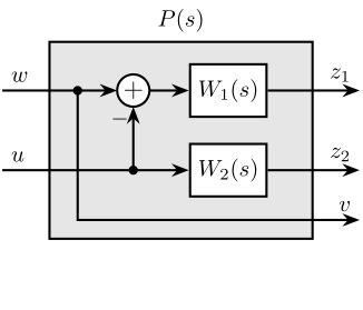
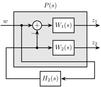
The synthesis objective can be easily expressed as a standard $\mathcal{H}_\infty$ optimization problem and therefore solved using convenient tools readily available. Consider the generalized plant $P(s)$ shown in Figure ref:fig:detail_control_h_infinity_robust_fusion_plant and mathematically described by eqref:eq:detail_control_generalized_plant.
\begin{equation}\label{eq:detail_control_generalized_plant} \begin{bmatrix} z_1 \\ z_2 \\ v \end{bmatrix} = P(s) \begin{bmatrix} w\\u \end{bmatrix}; \quad P(s) = \begin{bmatrix}W_1(s) & -W_1(s) \\ 0 & \phantom{+}W_2(s) \\ 1 & 0 \end{bmatrix} = P(s) \begin{bmatrix} w\\u \end{bmatrix}; \quad P(s) = \begin{bmatrix}W_1(s) & -W_1(s) \\ 0 & \phantom{+}W_2(s) \\ 1 & 0 \end{bmatrix}; \quad P(s) = \begin{bmatrix}W_1(s) & -W_1(s) \\ 0 & \phantom{+}W_2(s) \\ 1 & 0 \end{bmatrix}
\end{equation}
\tikzset{block/.default={0.8cm}{0.8cm}}
\tikzset{addb/.append style={scale=0.7}}
\tikzset{node distance=0.6}
\begin{tikzpicture}
  \node[block={4.0cm}{3.0cm}, fill=black!10!white] (P) {};
  \node[above] at (P.north) {$P(s)$};

  \node[block, below=0.2 of P, opacity=0] (H2) {$H_2(s)$};

  \coordinate[] (inputw)  at ($(P.south west)!0.75!(P.north west) + (-0.7, 0)$);
  \coordinate[] (inputu)  at ($(P.south west)!0.35!(P.north west) + (-0.7, 0)$);

  \coordinate[] (output1) at ($(P.south east)!0.75!(P.north east) + ( 0.7, 0)$);
  \coordinate[] (output2) at ($(P.south east)!0.35!(P.north east) + ( 0.7, 0)$);
  \coordinate[] (outputv) at ($(P.south east)!0.1!(P.north east) + ( 0.7, 0)$);

  \node[block, left=1.4 of output1] (W1){$W_1(s)$};
  \node[block, left=1.4 of output2] (W2){$W_2(s)$};
  \node[addb={+}{}{}{}{-}, left=of W1] (sub) {};

  \draw[->] (inputw) node[above right]{$w$} -- (sub.west);
  \draw[->] (inputu) node[above right]{$u$} -- (W2.west);
  \draw[->] (inputu-|sub) node[branch]{} -- (sub.south);
  \draw[->] (sub.east) -- (W1.west);
  \draw[->] ($(sub.west)+(-0.6, 0)$) node[branch]{} |- (outputv) node[above left]{$v$};
  \draw[->] (W1.east) -- (output1)node[above left]{$z_1$};
  \draw[->] (W2.east) -- (output2)node[above left]{$z_2$};
\end{tikzpicture}\tikzset{block/.default={0.8cm}{0.8cm}}
\tikzset{addb/.append style={scale=0.7}}
\tikzset{node distance=0.6}
\begin{tikzpicture}
\node[block={4.0cm}{3.0cm}, fill=black!10!white] (P) {};
\node[above] at (P.north) {$P(s)$};
\node[block, below=0.2 of P] (H2) {$H_2(s)$};
\coordinate[] (inputw) at ($(P.south west)!0.75!(P.north west) + (-0.7, 0)$);
\coordinate[] (inputu) at ($(P.south west)!0.35!(P.north west) + (-0.4, 0)$);
\coordinate[] (output1) at ($(P.south east)!0.75!(P.north east) + ( 0.7, 0)$);
\coordinate[] (output2) at ($(P.south east)!0.35!(P.north east) + ( 0.7, 0)$);
\coordinate[] (outputv) at ($(P.south east)!0.1!(P.north east) + ( 0.4, 0)$);
\node[block, left=1.4 of output1] (W1){$W_1(s)$};
\node[block, left=1.4 of output2] (W2){$W_2(s)$};
\node[addb={+}{}{}{}{-}, left=of W1] (sub) {};
\draw[->] (inputw) node[above right]{$w$} -- (sub.west);
\draw[->] (inputu-|sub) node[branch]{} -- (sub.south);
\draw[->] (sub.east) -- (W1.west);
\draw[->] ($(sub.west)+(-0.6, 0)$) node[branch]{} |- (outputv) |- (H2.east);
\draw[->] (H2.west) -| (inputu) -- (W2.west);
\draw[->] (W1.east) -- (output1)node[above left]{$z_1$};
\draw[->] (W2.east) -- (output2)node[above left]{$z_2$};
\end{tikzpicture}Applying the standard $\mathcal{H}_\infty$ synthesis to the generalized plant $P(s)$ is then equivalent as finding a stable filter $H_2(s)$ which based on $v$, generates a signal $u$ such that the $\mathcal{H}_\infty$ norm of the system in Figure ref:fig:detail_control_h_infinity_robust_fusion_fb from $w$ to $[z_1, \ z_2]$ is less than one eqref:eq:detail_control_hinf_syn_obj.
\begin{equation}\label{eq:detail_control_hinf_syn_obj} ≤ft\|\begin{matrix} \left(1 - H_2(s)\right) W_1(s) \\ H_2(s) W_2(s) \end{matrix}\right\|_∞ ≤ 1
\end{equation}
By then defining $H_1(s)$ to be the complementary of $H_2(s)$ eqref:eq:detail_control_definition_H1, the $\mathcal{H}_\infty$ synthesis objective becomes equivalent to eqref:eq:detail_control_hinf_problem which ensures that eqref:eq:detail_control_hinf_cond_h1 and eqref:eq:detail_control_hinf_cond_h2 are satisfied.
\begin{equation}\label{eq:detail_control_definition_H1} H_1(s) ≜ 1 - H_2(s)
\end{equation}
\begin{equation}\label{eq:detail_control_hinf_problem} ≤ft\|\begin{matrix} H_1(s) W_1(s) \\ H_2(s) W_2(s) \end{matrix}\right\|_∞ ≤ 1
\end{equation}
Therefore, applying the $\mathcal{H}_\infty$ synthesis to the standard plant $P(s)$ eqref:eq:detail_control_generalized_plant will generate two filters $H_2(s)$ and $H_1(s) \triangleq 1 - H_2(s)$ that are complementary eqref:eq:detail_control_comp_filter_problem_form and such that there norms are bellow specified bounds eqref:eq:detail_control_hinf_cond_h1, eqref:eq:detail_control_hinf_cond_h2.
Note that there is only an implication between the $\mathcal{H}_\infty$ norm condition eqref:eq:detail_control_hinf_problem and the initial synthesis objectives eqref:eq:detail_control_hinf_cond_h1 and eqref:eq:detail_control_hinf_cond_h2 and not an equivalence. Hence, the optimization may be a little bit conservative with respect to the set of filters on which it is performed, see cite:&skogestad07_multiv_feedb_contr,Chap. 2.8.3.
Weighting Functions Design
Weighting functions are used during the synthesis to specify the maximum allowed complementary filters' norm. The proper design of these weighting functions is of primary importance for the success of the presented $\mathcal{H}_\infty$ synthesis of complementary filters.
First, only proper and stable transfer functions should be used. Second, the order of the weighting functions should stay reasonably small in order to reduce the computational costs associated with the solving of the optimization problem and for the physical implementation of the filters (the synthesized filters' order being equal to the sum of the weighting functions' order). Third, one should not forget the fundamental limitations imposed by the complementary property eqref:eq:detail_control_comp_filter. This implies for instance that $|H_1(j\omega)|$ and $|H_2(j\omega)|$ cannot be made small at the same frequency.
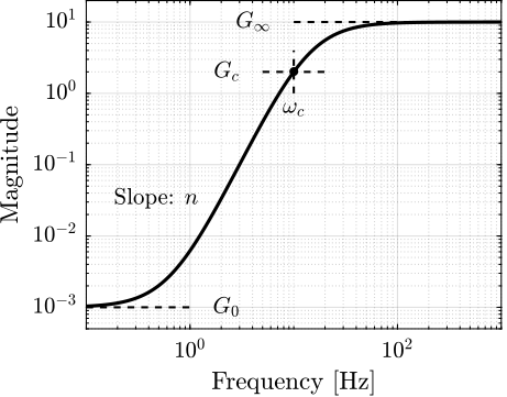
When designing complementary filters, it is usually desired to specify their slopes, their "blending" frequency and their maximum gains at low and high frequency. To easily express these specifications, formula eqref:eq:detail_control_weight_formula is proposed to help with the design of weighting functions. The parameters in formula eqref:eq:detail_control_weight_formula are $G_0 = \lim_{\omega \to 0} |W(j\omega)|$ the low frequency gain, $G_\infty = \lim_{\omega \to \infty} |W(j\omega)|$ the high frequency gain, $G_c = |W(j\omega_c)|$ the gain at a specific frequency $\omega_c$ in $\si{rad/s}$ and $n$ the slope between high and low frequency, which also corresponds to the order of the weighting function. The typical magnitude of a weighting function generated using eqref:eq:detail_control_weight_formula is shown in Figure ref:fig:detail_control_weight_formula.
\hfill
\begin{equation}\label{eq:detail_control_weight_formula} W(s) = ≤ft( \frac{ \hfill{} \frac{1}{ω_c} \sqrt{\frac{1 - ≤ft(\frac{G_0}{G_c}\right)^{\frac{2}{n}}}{1 - ≤ft(\frac{G_c}{G_∞}\right)^{\frac{2}{n}}}} s + ≤ft(\frac{G_0}{G_c}\right)^{\frac{1}{n}} }{ ≤ft(\frac{1}{G_∞}\right)^{\frac{1}{n}} \frac{1}{ω_c} \sqrt{\frac{1 - ≤ft(\frac{G_0}{G_c}\right)^{\frac{2}{n}}}{1 - ≤ft(\frac{G_c}{G_∞}\right)^{\frac{2}{n}}}} s + ≤ft(\frac{1}{G_c}\right)^{\frac{1}{n}} }\right)^n
\end{equation}
Validation of the proposed synthesis method
The proposed methodology for the design of complementary filters is now applied on a simple example. Let's suppose two complementary filters $H_1(s)$ and $H_2(s)$ have to be designed such that:
- the blending frequency is around $\SI{10}{Hz}$.
- the slope of $|H_1(j\omega)|$ is $+2$ below $\SI{10}{Hz}$. Its low frequency gain is $10^{-3}$.
- the slope of $|H_2(j\omega)|$ is $-3$ above $\SI{10}{Hz}$. Its high frequency gain is $10^{-3}$.
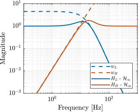
The first step is to translate the above requirements by properly designing the weighting functions. The proposed formula eqref:eq:detail_control_weight_formula is here used for such purpose. Parameters used are summarized in Table ref:tab:detail_control_weights_params. The inverse magnitudes of the designed weighting functions, which are representing the maximum allowed norms of the complementary filters, are shown by the dashed lines in Figure ref:fig:detail_control_hinf_filters_results.
%% Synthesis of Complementary Filters using H-infinity synthesis
% Design of the Weighting Functions
W1 = generateWF('n', 3, 'w0', 2*pi*10, 'G0', 1000, 'Ginf', 1/10, 'Gc', 0.45);
W2 = generateWF('n', 2, 'w0', 2*pi*10, 'G0', 1/10, 'Ginf', 1000, 'Gc', 0.45);

% Generalized Plant
P = [W1 -W1;
     0   W2;
     1   0];

% H-Infinity Synthesis
[H2, ~, gamma, ~] = hinfsyn(P, 1, 1,'TOLGAM', 0.001, 'METHOD', 'ric', 'DISPLAY', 'on');

% Define H1 to be the complementary of H2
H1 = 1 - H2;

% The function generateCF can also be used to synthesize the complementary filters.
% [H1, H2] = generateCF(W1, W2);| Parameter | $W_1(s)$ | $W_2(s)$ |
|---|---|---|
| $G_0$ | $0.1$ | $1000$ |
| $G_{\infty}$ | $1000$ | $0.1$ |
| $\omega_c$ | $2 \pi \cdot 10$ | $2 \pi \cdot 10$ |
| $G_c$ | $0.45$ | $0.45$ |
| $n$ | $2$ | $3$ |
\hfill
The standard $\mathcal{H}_\infty$ synthesis is then applied to the generalized plant of Figure ref:fig:detail_control_h_infinity_robust_fusion_plant. The filter $H_2(s)$ that minimizes the $\mathcal{H}_\infty$ norm between $w$ and $[z_1,\ z_2]^T$ is obtained. The $\mathcal{H}_\infty$ norm is here found to be close to one which indicates that the synthesis is successful: the complementary filters norms are below the maximum specified upper bounds. This is confirmed by the bode plots of the obtained complementary filters in Figure ref:fig:detail_control_hinf_filters_results. This simple example illustrates the fact that the proposed methodology for complementary filters shaping is easy to use and effective.
Synthesis of a set of three complementary filters
<<sec:detail_control_hinf_three_comp_filters>>
Some applications may require to merge more than two sensors cite:&stoten01_fusion_kinet_data_using_compos_filter;&fonseca15_compl. For instance at the LIGO, three sensors (an LVDT, a seismometer and a geophone) are merged to form a super sensor cite:&matichard15_seism_isolat_advan_ligo.
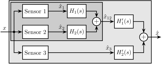
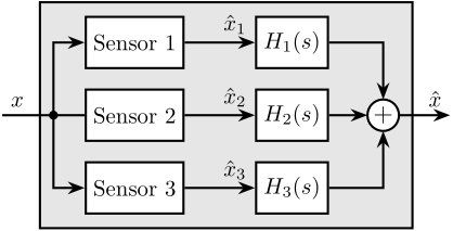
When merging $n>2$ sensors using complementary filters, two architectures can be used as shown in Figure ref:fig:detail_control_sensor_fusion_three. The fusion can either be done in a "sequential" way where $n-1$ sets of two complementary filters are used (Figure ref:fig:detail_control_sensor_fusion_three_sequential), or in a "parallel" way where one set of $n$ complementary filters is used (Figure ref:fig:detail_control_sensor_fusion_three_parallel).
In the first case, typical sensor fusion synthesis techniques can be used. However, when a parallel architecture is used, a new synthesis method for a set of more than two complementary filters is required as only simple analytical formulas have been proposed in the literature cite:&stoten01_fusion_kinet_data_using_compos_filter;&fonseca15_compl. A generalization of the proposed synthesis method of complementary filters is presented in this section.
\tikzset{block/.default={0.8cm}{0.8cm}}
\tikzset{addb/.append style={scale=0.7}}
\tikzset{node distance=0.6}
\begin{tikzpicture}
  \node[branch] (x) at (0, 0);

  \node[block, right=0.4 of x] (sensor2) {Sensor 2};
  \node[block, above=0.4 of sensor2] (sensor1) {Sensor 1};
  \node[block, below=0.4 of sensor2] (sensor3) {Sensor 3};

  \node[block, right=1.1 of sensor1](H1){$H_1(s)$};
  \node[block, right=1.1 of sensor2](H2){$H_2(s)$};
  \node[addb] (add) at ($0.5*(H1.east)+0.5*(H2.east)+(0.6, 0)$){};

  \node[block, right=0.8 of add](H1p)  {$H_1^\prime(s)$};
  \node[block] (H2p) at (H1p|-sensor3) {$H_2^\prime(s)$};

  \node[addb] (addp) at ($0.5*(H1p.east)+0.5*(H2p.east)+(0.6, 0)$){};

  \draw[->] ($(x)+(-0.8, 0)$) node[above right]{$x$} -- (sensor2.west);
  \draw[->] (x.center)     |- (sensor1.west);
  \draw[->] (x.center)     |- (sensor3.west);
  \draw[->] (sensor1.east) -- (H1.west)  node[above left]{$\hat{x}_1$};
  \draw[->] (sensor2.east) -- (H2.west)  node[above left]{$\hat{x}_2$};
  \draw[->] (sensor3.east) -- (H2p.west) node[above left]{$\hat{x}_3$};
  \draw[->] (H1)           -| (add.north);
  \draw[->] (H2)           -| (add.south);
  \draw[->] (add.east)     -- (H1p.west) node[above left]{$\hat{x}_{12}$};
  \draw[->] (H1p)          -| (addp.north);
  \draw[->] (H2p)          -| (addp.south);
  \draw[->] (addp.east)    -- ++(0.8, 0) node[above left]{$\hat{x}$};

  \begin{scope}[on background layer]
    \node[fit={(x.west|-sensor3.south) (sensor1.north-|addp.east)}, fill=black!10!white, draw, inner sep=6pt] (supersensor) {};

    \node[fit={(x.west|-sensor1.north) (add.east|-sensor2.south)}, fill=black!20!white, draw, inner sep=3pt] (superinertialsensor) {};
  \end{scope}
\end{tikzpicture}\tikzset{block/.default={0.8cm}{0.8cm}}
\tikzset{addb/.append style={scale=0.7}}
\tikzset{node distance=0.6}
\begin{tikzpicture}
\node[branch] (x) at (0, 0);
\node[block, right=0.4 of x] (sensor2) {Sensor 2};
\node[block, above=0.3 of sensor2] (sensor1) {Sensor 1};
\node[block, below=0.3 of sensor2] (sensor3) {Sensor 3};
\node[block, right=1.1 of sensor1](H1){$H_1(s)$};
\node[block, right=1.1 of sensor2](H2){$H_2(s)$};
\node[block, right=1.1 of sensor3](H3){$H_3(s)$};
\node[addb, right=0.6 of H2](add){};
\draw[->] (x.center) |- (sensor1.west);
\draw[] ($(x)+(-0.8, 0)$) node[above right]{$x$} -- (sensor2.west);
\draw[->] (x.center) |- (sensor3.west);
\draw[->] (sensor1.east) -- (H1.west) node[above left]{$\hat{x}_1$};
\draw[->] (sensor2.east) -- (H2.west) node[above left]{$\hat{x}_2$};
\draw[->] (sensor3.east) -- (H3.west) node[above left]{$\hat{x}_3$};
\draw[->] (H1) -| (add.north);
\draw[->] (H2) -- (add.west);
\draw[->] (H3) -| (add.south);
\draw[->] (add.east) -- ++(0.8, 0) node[above left]{$\hat{x}$};
\begin{scope}[on background layer]
\node[fit={(H3.south-|x) (H1.north-|add.east)}, fill=black!10!white, draw, inner sep=6pt] (supersensor) {};
\end{scope}
\end{tikzpicture}The synthesis objective is to compute a set of $n$ stable transfer functions $[H_1(s),\ H_2(s),\ \dots,\ H_n(s)]$ such that conditions eqref:eq:detail_control_hinf_cond_compl_gen and eqref:eq:detail_control_hinf_cond_perf_gen are satisfied.
\begin{subequations}\label{eq:detail_control_hinf_problem_gen}
\begin{align} & \sum_{i=1}^n H_i(s) = 1 \label{eq:detail_control_hinf_cond_compl_gen} \\ & \left| H_i(j\omega) \right| < \frac{1}{\left| W_i(j\omega) \right|}, \quad \forall \omega,\ i = 1 \dots n \label{eq:detail_control_hinf_cond_perf_gen} \end{align}\end{subequations}
$[W_1(s),\ W_2(s),\ \dots,\ W_n(s)]$ are weighting transfer functions that are chosen to specify the maximum complementary filters' norm during the synthesis.
Such synthesis objective is closely related to the one described in Section ref:ssec:detail_control_hinf_method, and indeed the proposed synthesis method is a generalization of the one previously presented. A set of $n$ complementary filters can be shaped by applying the standard $\mathcal{H}_\infty$ synthesis to the generalized plant $P_n(s)$ described by eqref:eq:detail_control_generalized_plant_n_filters.
\begin{equation}\label{eq:detail_control_generalized_plant_n_filters}
\begin{bmatrix} z_1 \\ \vdots \\ z_n \\ v \end{bmatrix} = P_n(s) \begin{bmatrix} w \\ u_1 \\ \vdots \\ u_{n-1} \end{bmatrix} = P_n(s) \begin{bmatrix} w \\ u_1 \\ \vdots \\ u_{n-1} \end{bmatrix}; \quad
P_n(s) = \begin{bmatrix}
W_1 & -W_1 & … & … & -W_1
0 & W_2 & 0 & … & 0
\vdots & \ddots & \ddots & \ddots & \vdots
\vdots & & \ddots & \ddots & 0
0 & … & … & 0 & W_n
1 & 0 & … & … & 0
\end{bmatrix}
\end{equation}
If the synthesis if successful, a set of $n-1$ filters $[H_2(s),\ H_3(s),\ \dots,\ H_n(s)]$ are obtained such that eqref:eq:detail_control_hinf_syn_obj_gen is verified.
\begin{equation}\label{eq:detail_control_hinf_syn_obj_gen} ≤ft\|\begin{matrix} \left(1 - \left[ H_2(s) + H_3(s) + \dots + H_n(s) \right]\right) W_1(s) \\ H_2(s) W_2(s) \\ \vdots \\ H_n(s) W_n(s) \end{matrix}\right\|_∞ ≤ 1
\end{equation}
$H_1(s)$ is then defined using eqref:eq:detail_control_h1_comp_h2_hn which is ensuring the complementary property for the set of $n$ filters eqref:eq:detail_control_hinf_cond_compl_gen. Condition eqref:eq:detail_control_hinf_cond_perf_gen is satisfied thanks to eqref:eq:detail_control_hinf_syn_obj_gen.
\begin{equation}\label{eq:detail_control_h1_comp_h2_hn} H_1(s) ≜ 1 - \big[ H_2(s) + H_3(s) + … + H_n(s) \big]
\end{equation}
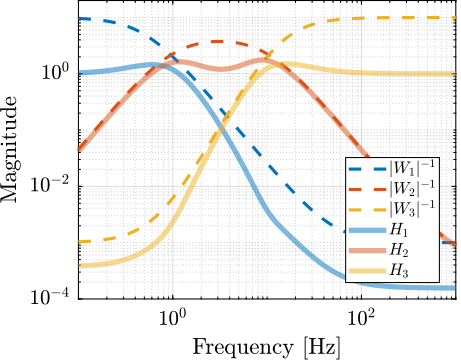
An example is given to validate the proposed method for the synthesis of a set of three complementary filters. The sensors to be merged are a displacement sensor from DC up to $\SI{1}{Hz}$, a geophone from $1$ to $\SI{10}{Hz}$ and an accelerometer above $\SI{10}{Hz}$. Three weighting functions are designed using formula eqref:eq:detail_control_weight_formula and their inverse magnitude are shown in Figure ref:fig:detail_control_three_complementary_filters_results (dashed curves).
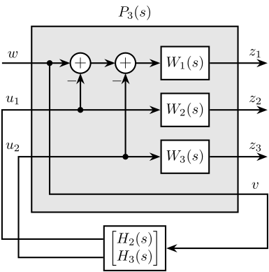
Consider the generalized plant $P_3(s)$ shown in Figure ref:fig:detail_control_comp_filter_three_hinf_fb which is also described by eqref:eq:detail_control_generalized_plant_three_filters.
\begin{equation}\label{eq:detail_control_generalized_plant_three_filters} \begin{bmatrix} z_1 \\ z_2 \\ z_3 \\ v \end{bmatrix} = P_3(s) \begin{bmatrix} w \\ u_1 \\ u_2 \end{bmatrix}; \quad P_3(s) = \begin{bmatrix}W_1(s) & -W_1(s) & -W_1(s) \\ 0 & \phantom{+}W_2(s) & 0 \\ 0 & 0 & \phantom{+}W_3(s) \\ 1 & 0 & 0 \end{bmatrix} = P_3(s) \begin{bmatrix} w \\ u_1 \\ u_2 \end{bmatrix}; \quad P_3(s) = \begin{bmatrix}W_1(s) & -W_1(s) & -W_1(s) \\ 0 & \phantom{+}W_2(s) & 0 \\ 0 & 0 & \phantom{+}W_3(s) \\ 1 & 0 & 0 \end{bmatrix}; \quad P_3(s) = \begin{bmatrix}W_1(s) & -W_1(s) & -W_1(s) \\ 0 & \phantom{+}W_2(s) & 0 \\ 0 & 0 & \phantom{+}W_3(s) \\ 1 & 0 & 0 \end{bmatrix}
\end{equation}
\tikzset{block/.default={0.8cm}{0.8cm}}
\tikzset{addb/.append style={scale=0.7}}
\tikzset{node distance=0.6}
\begin{tikzpicture}
  \node[block={5.0cm}{4.5cm}, fill=black!10!white] (P) {};
  \node[above] at (P.north) {$P_3(s)$};

  \coordinate[] (inputw)  at ($(P.south west)!0.8!(P.north west) + (-0.7, 0)$);
  \coordinate[] (inputu)  at ($(P.south west)!0.4!(P.north west) + (-0.7, 0)$);

  \coordinate[] (output1) at ($(P.south east)!0.8!(P.north east)  + (0.7, 0)$);
  \coordinate[] (output2) at ($(P.south east)!0.55!(P.north east) + (0.7, 0)$);
  \coordinate[] (output3) at ($(P.south east)!0.3!(P.north east)  + (0.7, 0)$);
  \coordinate[] (outputv) at ($(P.south east)!0.1!(P.north east)  + (0.7, 0)$);

  \node[block, left=1.4 of output1] (W1){$W_1(s)$};
  \node[block, left=1.4 of output2] (W2){$W_2(s)$};
  \node[block, left=1.4 of output3] (W3){$W_3(s)$};
  \node[addb={+}{}{}{}{-}, left=of W1] (sub1) {};
  \node[addb={+}{}{}{}{-}, left=of sub1] (sub2) {};

  \node[block, below=0.3 of P, opacity=0] (H) {$\begin{bmatrix}H_2(s) \\ H_3(s)\end{bmatrix}$};

  \draw[->] (inputw) node[above right](w){$w$} -- (sub2.west);
  \draw[->] (W3-|sub1)node[branch]{} -- (sub1.south);
  \draw[->] (W2-|sub2)node[branch]{} -- (sub2.south);
  \draw[->] ($(sub2.west)+(-0.5, 0)$) node[branch]{} |- (outputv);
  \draw[->] (inputu|-W2) -- (W2.west);
  \draw[->] (inputu|-W3) -- (W3.west);

  \draw[->] (sub2.east) -- (sub1.west);
  \draw[->] (sub1.east) -- (W1.west);
  \draw[->] (W1.east) -- (output1)node[above left](z){$z_1$};
  \draw[->] (W2.east) -- (output2)node[above left]{$z_2$};
  \draw[->] (W3.east) -- (output3)node[above left]{$z_3$};
  \node[above] at (W2-|w){$u_1$};
  \node[above] at (W3-|w){$u_2$};
  \node[above] at (outputv-|z){$v$};
\end{tikzpicture}\tikzset{block/.default={0.8cm}{0.8cm}}
\tikzset{addb/.append style={scale=0.7}}
\tikzset{node distance=0.6}
\begin{tikzpicture}
\node[block={5.0cm}{4.5cm}, fill=black!10!white] (P) {};
\node[above] at (P.north) {$P_3(s)$};
\coordinate[] (inputw) at ($(P.south west)!0.8!(P.north west) + (-0.7, 0)$);
\coordinate[] (inputu) at ($(P.south west)!0.4!(P.north west) + (-0.7, 0)$);
\coordinate[] (output1) at ($(P.south east)!0.8!(P.north east) + (0.7, 0)$);
\coordinate[] (output2) at ($(P.south east)!0.55!(P.north east) + (0.7, 0)$);
\coordinate[] (output3) at ($(P.south east)!0.3!(P.north east) + (0.7, 0)$);
\coordinate[] (outputv) at ($(P.south east)!0.1!(P.north east) + (0.7, 0)$);
\node[block, left=1.4 of output1] (W1){$W_1(s)$};
\node[block, left=1.4 of output2] (W2){$W_2(s)$};
\node[block, left=1.4 of output3] (W3){$W_3(s)$};
\node[addb={+}{}{}{}{-}, left=of W1] (sub1) {};
\node[addb={+}{}{}{}{-}, left=of sub1] (sub2) {};
\node[block, below=0.3 of P] (H) {$\begin{bmatrix}H_2(s) \\ H_3(s)\end{bmatrix}$};
\draw[->] (inputw) node[above right](w){$w$} -- (sub2.west);
\draw[->] (W3-|sub1)node[branch]{} -- (sub1.south);
\draw[->] (W2-|sub2)node[branch]{} -- (sub2.south);
\draw[->] ($(sub2.west)+(-0.5, 0)$) node[branch]{} |- (outputv) |- (H.east);
\draw[->] ($(H.south west)!0.7!(H.north west)$) -| (inputu|-W2) -- (W2.west);
\draw[->] ($(H.south west)!0.3!(H.north west)$) -| ($(inputu|-W3)+(0.4, 0)$) -- (W3.west);
\draw[->] (sub2.east) -- (sub1.west);
\draw[->] (sub1.east) -- (W1.west);
\draw[->] (W1.east) -- (output1)node[above left](z){$z_1$};
\draw[->] (W2.east) -- (output2)node[above left]{$z_2$};
\draw[->] (W3.east) -- (output3)node[above left]{$z_3$};
\node[above] at (W2-|w){$u_1$};
\node[above] at (W3-|w){$u_2$};
\node[above] at (outputv-|z){$v$};
\end{tikzpicture}The standard $\mathcal{H}_\infty$ synthesis is performed on the generalized plant $P_3(s)$. Two filters $H_2(s)$ and $H_3(s)$ are obtained such that the $\mathcal{H}_\infty$ norm of the closed-loop transfer from $w$ to $[z_1,\ z_2,\ z_3]$ of the system in Figure ref:fig:detail_control_comp_filter_three_hinf_fb is less than one. Filter $H_1(s)$ is defined using eqref:eq:detail_control_h1_compl_h2_h3 thus ensuring the complementary property of the obtained set of filters.
\begin{equation}\label{eq:detail_control_h1_compl_h2_h3} H_1(s) ≜ 1 - \big[ H_2(s) + H_3(s) \big]
\end{equation}
Figure ref:fig:detail_control_three_complementary_filters_results displays the three synthesized complementary filters (solid lines) which confirms that the synthesis is successful.
%% Synthesis of a set of three complementary filters
% Design of the Weighting Functions
W1 = generateWF('n', 2, 'w0', 2*pi*1, 'G0', 1/10, 'Ginf', 1000, 'Gc', 0.5);
W2 = 0.22*(1 + s/2/pi/1)^2/(sqrt(1e-4) + s/2/pi/1)^2*(1 + s/2/pi/10)^2/(1 + s/2/pi/1000)^2;
W3 = generateWF('n', 3, 'w0', 2*pi*10, 'G0', 1000, 'Ginf', 1/10, 'Gc', 0.5);

% Generalized plant for the synthesis of 3 complementary filters
P = [W1 -W1 -W1;
     0   W2  0 ;
     0   0   W3;
     1   0   0];

% Standard H-Infinity Synthesis
[H, ~, gamma, ~] = hinfsyn(P, 1, 2,'TOLGAM', 0.001, 'METHOD', 'ric', 'DISPLAY', 'on');

% Synthesized H2 and H3 filters
H2 = tf(H(1));
H3 = tf(H(2));

% H1 is defined as the complementary filter of H2 and H3
H1 = 1 - H2 - H3;
TODO Conclusion
A new method for designing complementary filters using the $\mathcal{H}_\infty$ synthesis has been proposed. It allows to shape the magnitude of the filters by the use of weighting functions during the synthesis. This is very valuable in practice as the characteristics of the super sensor are linked to the complementary filters' magnitude. Therefore typical sensor fusion objectives can be translated into requirements on the magnitudes of the filters. Several examples were used to emphasize the simplicity and the effectiveness of the proposed method.
However, the shaping of the complementary filters' magnitude does not allow to directly optimize the super sensor noise and dynamical characteristics. Future work will aim at developing a complementary filter synthesis method that minimizes the super sensor noise while ensuring the robustness of the fusion.
- Talk about the possibility to use H2 to minimize the RMS value of the super sensor noise? (or maybe make a section about that?) There is a draft paper about that.
- For the NASS, it was shown that the HAC-IFF strategy works fine and is easy to understand and tune
- It would be very interesting to see how sensor fusion (probably between the force sensor and the external metrology) compares in term of performance and robustness
TODO [A] Decoupling
<<sec:detail_control_decoupling>>
Introduction ignore
When dealing with MIMO systems, a typical strategy is to:
- First decouple the plant dynamics (discussed in this section)
- Apply SISO control for the decoupled plant (discussed in section ref:sec:detail_control_optimization)
Another strategy would be to apply a multivariable control synthesis to the coupled system. Strangely, while H-infinity synthesis is a mature technology, it use for the control of Stewart platform is not yet demonstrated. From cite:&thayer02_six_axis_vibrat_isolat_system:
Experimental closed-loop control results using the hexapod have shown that controllers designed using a decentralized single-strut design work well when compared to full multivariable methodologies.
- Review of Decoupling Strategies for stewart platforms
- Add some citations about different methods
- Maybe transform table into text
| Actuators | Sensors | Control | Reference |
|---|---|---|---|
| APA | Eddy current displacement | Decentralized (struts) PI + LPF control | cite:&furutani04_nanom_cuttin_machin_using_stewar |
| PZT Piezo | Strain Gauge | Decentralized position feedback | cite:&du14_piezo_actuat_high_precis_flexib |
| Voice Coil | Force | Cartesian frame decoupling | cite:&obrien98_lesson |
| Voice Coil | Force | Cartesian Frame, Jacobians, IFF | cite:&mcinroy99_dynam;&mcinroy99_precis_fault_toler_point_using_stewar_platf;&mcinroy00_desig_contr_flexur_joint_hexap |
| Hydraulic | LVDT | Decentralized (strut) vs Centralized (cartesian) | cite:&kim00_robus_track_contr_desig_dof_paral_manip |
| Voice Coil | Accelerometer (collocated), ext. Rx/Ry sensors | Cartesian acceleration feedback (isolation) + 2DoF pointing control (external sensor) | cite:&li01_simul_vibrat_isolat_point_contr |
| Voice Coil | Accelerometer in each leg | Centralized Vibration Control, PI, Skyhook | cite:&abbas14_vibrat_stewar_platf |
| Voice Coil | Geophone + Eddy Current (Struts, collocated) | Decentralized (Sky Hook) + Centralized (modal) Control | cite:&pu11_six_degree_of_freed_activ |
| Piezoelectric | Force, Position | Vibration isolation, Model-Based, Modal control: 6x PI controllers | cite:&yang19_dynam_model_decoup_contr_flexib |
| PZT | Geophone (struts) | H-Infinity and mu-synthesis | cite:&lei08_multi_objec_robus_activ_vibrat |
| Voice Coil | Force sensors (struts) + accelerometer (cartesian) | Decentralized Force Feedback + Centralized H2 control based on accelerometers | cite:&xie17_model_contr_hybrid_passiv_activ |
| Voice Coil | Accelerometers | MIMO H-Infinity, active damping | cite:&jiao18_dynam_model_exper_analy_stewar |
The goal of this section is to compare the use of several methods for the decoupling of parallel manipulators.
It is structured as follow:
- Section ref:ssec:detail_control_decoupling_comp_model: the model used to compare/test decoupling strategies is presented
- Section ref:ssec:detail_control_comp_jacobian: decoupling using Jacobian matrices is presented
- Section ref:ssec:detail_control_comp_modal: modal decoupling is presented
- Section ref:ssec:detail_control_comp_svd: SVD decoupling is presented
- Section ref:ssec:detail_control_decoupling_comp: the three decoupling methods are applied on the test model and compared
- Conclusions are drawn on the three decoupling methods
Test Model
<<ssec:detail_control_decoupling_comp_model>>
- Instead of comparing the decoupling strategies using the Stewart platform, a similar yet much simpler parallel manipulator is used instead
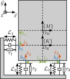
- to render the analysis simpler, the system of Figure ref:fig:detail_control_model_test_decoupling_detail is used
- It has 3DoF, and has 3 parallels struts whose model is shown in Figure ref:fig:detail_control_strut_model
- It is quite similar to the Stewart platform (parallel architecture, as many struts as DoF)
Two frames are defined:
- $\{M\}$ with origin $O_M$ at the Center of mass of the solid body
- $\{K\}$ with origin $O_K$ at the Center of mass of the parallel manipulator
First, the equation of motion are derived. Expressing the second law of Newton on the suspended mass, expressed at its center of mass gives
\begin{equation} M_{\{M\}} \ddot{\bm{\mathcal{X}}}_{\{M\}}(t) = \sum \bm{\mathcal{F}}_{\{M\}}(t) \end{equation}with $\bm{\mathcal{X}}_{\{M\}}$ the two translation and one rotation expressed with respect to the center of mass and $\bm{\mathcal{F}}_{\{M\}}$ forces and torque applied at the center of mass.
\begin{equation} \bm{\mathcal{X}}_{\{M\}} = \begin{bmatrix} x \\ y \\ R_z \end{bmatrix}, \quad \bm{\mathcal{F}}_{\{M\}} = \begin{bmatrix} F_x \\ F_y \\ M_z \end{bmatrix} \end{equation}In order to map the spring, damping and actuator forces to XY forces and Z torque expressed at the center of mass, the Jacobian matrix $\bm{J}_{\{M\}}$ is used.
\begin{equation}\label{eq:detail_control_decoupling_jacobian_CoM}
\bm{J}_{\{M\}} = \begin{bmatrix}
1 & 0 & h_a
0 & 1 & -l_a
0 & 1 & l_a \\
\end{bmatrix}
\end{equation}
Then, the equation of motion linking the actuator forces $\tau$ to the motion of the mass $\bm{\mathcal{X}}_{\{M\}}$ is obtained.
\begin{equation}\label{eq:detail_control_decoupling_plant_cartesian} M_{\{M\}} \ddot{\bm{\mathcal{X}}}_{\{M\}}(t) + \bm{J}_{\{M\}}^t \bm{\mathcal{C}} \bm{J}_{\{M\}} \dot{\bm{\mathcal{X}}}_{\{M\}}(t) + \bm{J}_{\{M\}}^t \bm{\mathcal{K}} \bm{J}_{\{M\}} \bm{\mathcal{X}}_{\{M\}}(t) = \bm{J}_{\{M\}}^t \bm{τ}(t)
\end{equation}
Matrices representing the payload inertia as well as the actuator stiffness and damping are shown in
\begin{equation} \bm{M}_{\{M\}} = \begin{bmatrix} m & 0 & 0 \\ 0 & m & 0 \\ 0 & 0 & I \end{bmatrix}, \quad \bm{\mathcal{K}} = \begin{bmatrix} k & 0 & 0 \\ 0 & k & 0 \\ 0 & 0 & k \end{bmatrix}, \quad \bm{\mathcal{C}} = \begin{bmatrix} c & 0 & 0 \\ 0 & c & 0 \\ 0 & 0 & c \end{bmatrix} \end{equation}Parameters used for the following analysis are summarized in table ref:tab:detail_control_decoupling_test_model_params.
| Parameter | Description | Value |
|---|---|---|
| $l_a$ | $0.5\,m$ | |
| $h_a$ | $0.2\,m$ | |
| $k$ | Actuator stiffness | $10\,N/\mu m$ |
| $c$ | Actuator damping | $200\,Ns/m$ |
| $m$ | Payload mass | $40\,\text{kg}$ |
| $I$ | Payload rotational inertia | $5\,\text{kg}m^2$ |
Control in the frame of the struts
Let's first study the obtained dynamics in the frame of the struts. The equation of motion linking actuator forces $\bm{\mathcal{\tau}}$ to strut relative motion $\bm{\mathcal{L}}$ is obtained from eqref:eq:detail_control_decoupling_plant_cartesian by mapping the cartesian motion of the mass to the relative motion of the struts using the Jacobian matrix $\bm{J}_{\{M\}}$ eqref:eq:detail_control_decoupling_jacobian_CoM .
The transfer function from $\bm{\mathcal{\tau}}$ to $\bm{\mathcal{L}}$ is shown in equation eqref:eq:detail_control_decoupling_plant_decentralized.
\begin{tikzpicture}
  \node[block] (Gl) {$\bm{G}_{\{\mathcal{L}\}}$};

  % Connections and labels
  \draw[<-] (Gl.west) -- ++(-0.8, 0) node[above right]{$\bm{\tau}$};
  \draw[->] (Gl.east) -- ++( 0.8, 0) node[above left]{$\bm{\mathcal{L}}$};
\end{tikzpicture}
\begin{equation}\label{eq:detail_control_decoupling_plant_decentralized} \frac{\bm{\mathcal{L}}}{\bm{\mathcal{τ}}}(s) = \bm{G}_{\mathcal{L}}(s) = ≤ft( \bm{J}_{\{M\}}-t M_{\{M\}} \bm{J}_{\{M\}}-1 s^2 + \bm{\mathcal{C}} s + \bm{\mathcal{K}} \right)-1
\end{equation}
At low frequency the plant converges to a diagonal constant matrix whose diagonal elements are linked to the actuator stiffnesses eqref:eq:detail_control_decoupling_plant_decentralized_low_freq.
\begin{equation}\label{eq:detail_control_decoupling_plant_decentralized_low_freq} \bm{G}_{\mathcal{L}}(jω) \xrightarrow[ω → 0]{} \bm{\mathcal{K}-1}
\end{equation}
At high frequency, the plant converges to the mass matrix mapped in the frame of the struts, which is in general highly non-diagonal.
%% Compute Equation of motion
l = 1; h=2;
la = 0.5; % Horizontal position of actuators [m]
ha = 0.2; % Vertical of actuators [m]

m = 40; % Payload mass [kg]
I = 5; % Payload rotational inertia [kg m^2]

% Actuator Damping [N/(m/s)]
c1 = 2e2;
c2 = 2e2;
c3 = 2e2;

% Actuator Stiffness [N/m]
k1 = 1e6;
k2 = 1e6;
k3 = 1e6;

% Unit vectors of the actuators
s1 = [1;0];
s2 = [0;1];
s3 = [0;1];

% Stiffnesss and Damping matrices of the struts
Kr = diag([k1,k2,k3]);
Cr = diag([c1,c2,c3]);

%  Location of the joints with respect to the center of mass
Mb1 = [-l/2;-ha];
Mb2 = [-la; -h/2];
Mb3 = [ la; -h/2];

% Jacobian matrix (Center of Mass)
J_CoM = [s1', Mb1(1)*s1(2)-Mb1(2)*s1(1);
         s2', Mb2(1)*s2(2)-Mb2(2)*s2(1);
         s3', Mb3(1)*s3(2)-Mb3(2)*s3(1)];

% Mass Matrix in frame {M}
M = diag([m,m,I]);

% Stiffness Matrix in frame {M}
K = J_CoM'*Kr*J_CoM;

% Damping Matrix in frame {M}
C = J_CoM'*Cr*J_CoM;

% Plant in the frame of the struts
G_L = J_CoM*inv(M*s^2 + C*s + K)*J_CoM';
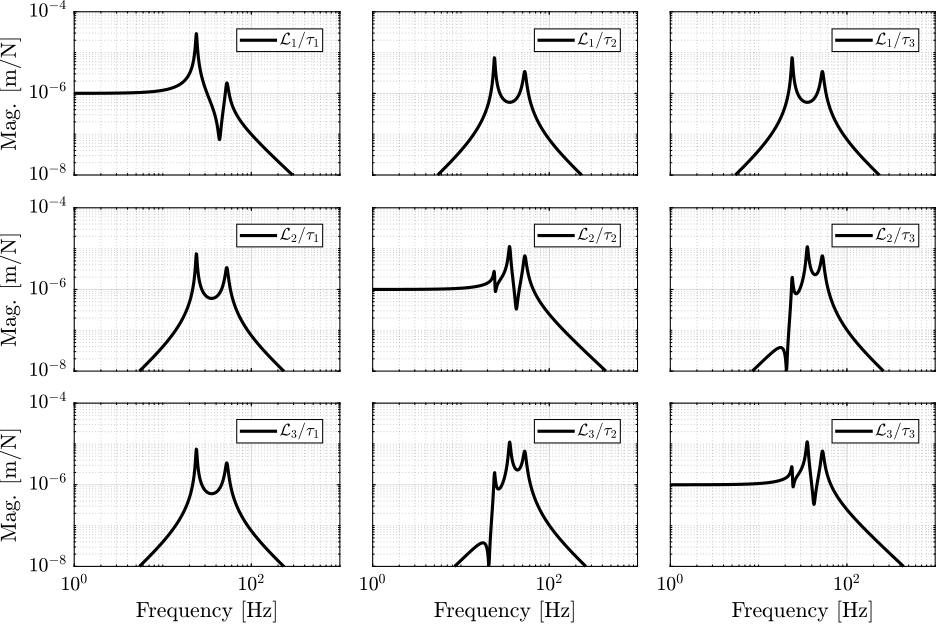
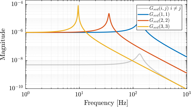
The magnitude of the coupled plant $\bm{G}_{\mathcal{L}}$ is shown in Figure ref:fig:detail_control_coupled_plant_bode. This confirms that at low frequency (below the first suspension mode), the plant is well decoupled. Depending on the symmetry in the system, some diagonal elements may be equal (such as for struts 2 and 3 in this example).
Jacobian Decoupling
<<ssec:detail_control_comp_jacobian>>
Jacobian Matrix
As already explained, the Jacobian matrix can be used to both convert strut velocity $\dot{\mathcal{L}}$ to payload velocity and angular velocity $\dot{\bm{\mathcal{X}}}_{\{O\}}$ and Convert actuators forces $\bm{\tau}$ to forces/torque applied on the payload $\bm{\mathcal{F}}_{\{O\}}$ eqref:eq:detail_control_decoupling_jacobian.
\begin{subequations}\label{eq:detail_control_decoupling_jacobian}
\begin{align} \dot{\bm{\mathcal{X}}}_{\{O\}} &= J_{\{O\}} \dot{\bm{\mathcal{L}}}, \quad \dot{\bm{\mathcal{L}}} = J_{\{O\}}^{-1} \dot{\bm{\mathcal{X}}}_{\{O\}} \\ \bm{\mathcal{F}}_{\{O\}} &= J_{\{O\}}^t \bm{\tau}, \quad \bm{\tau} = J_{\{O\}}^{-t} \bm{\mathcal{F}}_{\{O\}} \end{align}\end{subequations}
The obtained plan (Figure ref:fig:detail_control_jacobian_decoupling_arch) has inputs and outputs that have physical meaning:
- $\bm{\mathcal{F}}_{\{O\}}$ are forces/torques applied on the payload at the origin of frame $\{O\}$
- $\bm{\mathcal{X}}_{\{O\}}$ are translations/rotation of the payload expressed in frame $\{O\}$
\begin{tikzpicture}
  \node[block] (G) {$\bm{G}_{\{\mathcal{L}\}}$};
  \node[block, left=0.6 of G] (Jt) {$J_{\{O\}}^{-T}$};
  \node[block, right=0.6 of G] (Ja) {$J_{\{O\}}^{-1}$};

  % Connections and labels
  \draw[<-] (Jt.west) -- ++(-1.4, 0) node[above right]{$\bm{\mathcal{F}}_{\{O\}}$};
  \draw[->] (Jt.east) -- (G.west)  node[above left]{$\bm{\tau}$};
  \draw[->] (G.east) -- (Ja.west)  node[above left]{$\bm{\mathcal{L}}$};
  \draw[->] (Ja.east) -- ++( 1.4, 0)  node[above left]{$\bm{\mathcal{X}}_{\{O\}}$};

  \begin{scope}[on background layer]
    \node[fit={(Jt.south west) (Ja.north east)}, fill=black!10!white, draw, dashed, inner sep=4pt] (Gx) {};
    \node[above] at (Gx.north) {$\bm{G}_{\{O\}}$};
  \end{scope}
\end{tikzpicture}\begin{equation}\label{eq:detail_control_decoupling_plant_jacobian} \frac{\bm{\mathcal{X}}_{\{O\}}}{\bm{\mathcal{F}}_{\{O\}}}(s) = \bm{G}_{\{O\}}(s) = ≤ft( \bm{J}_{\{O\}}^t \bm{J}_{\{M\}}-T \bm{M}_{\{M\}} \bm{J}_{\{M\}}-1 \bm{J}_{\{O\}} s^2 + \bm{J}_{\{O\}}^t \bm{\mathcal{C}} \bm{J}_{\{O\}} s + \bm{J}_{\{O\}}^t \bm{\mathcal{K}} \bm{J}_{\{O\}} \right)-1
\end{equation}
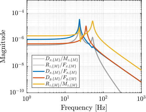
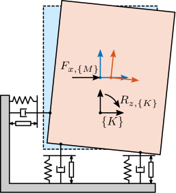
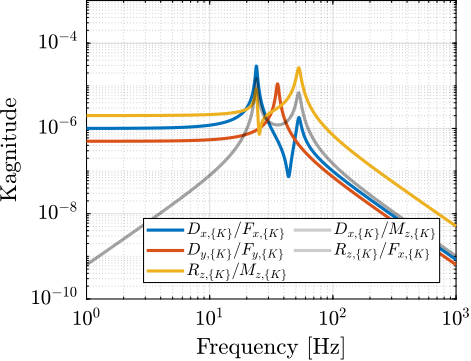
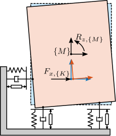
The frame $\{O\}$ can be any chosen frame, but the decoupling properties depends on the chosen frame $\{O\}$. There are two natural choices: the center of mass $\{M\}$ and the center of stiffness $\{K\}$. Note that the Jacobian matrix is only based on the geometry of the system and does not depend on the physical properties such as mass and stiffness.
Center Of Mass
If the center of mass is chosen as the decoupling frame. The Jacobian matrix and its inverse are expressed in eqref:eq:detail_control_decoupling_jacobian_CoM_inverse.
\begin{equation}\label{eq:detail_control_decoupling_jacobian_CoM_inverse}
J_{\{M\}} = \begin{bmatrix}
1 & 0 & h_a \\
0 & 1 & -l_a \\
0 & 1 & l_a \\
\end{bmatrix}, \quad J_{\{M\}}-1 = \begin{bmatrix}
1 & \frac{h_a}{2 l_a} & \frac{-h_a}{2 l_a}
0 & \frac{1}{2} & \frac{1}{2}
0 & \frac{-1}{2 l_a} & \frac{1}{2 l_a} \\
\end{bmatrix}
\end{equation}
\begin{tikzpicture}
  \node[block] (G) {$\bm{G}_{\{\mathcal{L}\}}$};
  \node[block, left=0.6 of G] (Jt) {$J_{\{M\}}^{-T}$};
  \node[block, right=0.6 of G] (Ja) {$J_{\{M\}}^{-1}$};

  % Connections and labels
  \draw[<-] (Jt.west) -- ++(-1.4, 0) node[above right]{$\bm{\mathcal{F}}_{\{M\}}$};
  \draw[->] (Jt.east) -- (G.west)  node[above left]{$\bm{\tau}$};
  \draw[->] (G.east) -- (Ja.west)  node[above left]{$\bm{\mathcal{L}}$};
  \draw[->] (Ja.east) -- ++( 1.4, 0)  node[above left]{$\bm{\mathcal{X}}_{\{M\}}$};

  \begin{scope}[on background layer]
    \node[fit={(Jt.south west) (Ja.north east)}, fill=black!10!white, draw, dashed, inner sep=4pt] (Gx) {};
    \node[above] at (Gx.north) {$\bm{G}_{\{M\}}$};
  \end{scope}
\end{tikzpicture}
Analytical formula of the plant is eqref:eq:detail_control_decoupling_plant_CoM.
\begin{equation}\label{eq:detail_control_decoupling_plant_CoM} \frac{\bm{\mathcal{X}}_{\{M\}}}{\bm{\mathcal{F}}_{\{M\}}}(s) = \bm{G}_{\{M\}}(s) = ≤ft( \bm{M}_{\{M\}} s^2 + \bm{J}_{\{M\}}^t \bm{\mathcal{C}} \bm{J}_{\{M\}} s + \bm{J}_{\{M\}}^t \bm{\mathcal{K}} \bm{J}_{\{M\}} \right)-1
\end{equation}
At high frequency, converges towards the inverse of the mass matrix, which is a diagonal matrix eqref:eq:detail_control_decoupling_plant_CoM_high_freq.
\begin{equation}\label{eq:detail_control_decoupling_plant_CoM_high_freq}
\bm{G}_{\{M\}}(jω) \xrightarrow[ω → ∞]{} -ω^2 \bm{M}_{\{M\}}-1 = -ω^2 \begin{bmatrix}
1/m & 0 & 0
0 & 1/m & 0
0 & 0 & 1/I
\end{bmatrix}
\end{equation}
Plant is therefore well decoupled above the suspension mode with the highest frequency. Such strategy is usually applied on systems with low frequency suspension modes, such that the plant corresponds to decoupled mass lines.
- Reference to some papers about vibration isolation or ASML?
The coupling at low frequency can easily be understood physically. When a static (or with frequency lower than the suspension modes) force is applied at the center of mass, rotation is induced by the stiffness of the first actuator, not in line with the force application point. this is illustrated in Figure ref:fig:detail_control_model_test_CoM.
%% Jacobian Decoupling - Center of Mass
G_CoM = pinv(J_CoM)*G_L*pinv(J_CoM');
G_CoM.InputName  = {'Fx', 'Fy', 'Mz'};
G_CoM.OutputName  = {'Dx', 'Dy', 'Rz'};
Center Of Stiffness
\begin{tikzpicture}
  \node[block] (G) {$\bm{G}_{\{\mathcal{L}\}}$};
  \node[block, left=0.6 of G] (Jt) {$J_{\{K\}}^{-T}$};
  \node[block, right=0.6 of G] (Ja) {$J_{\{K\}}^{-1}$};

  % Connections and labels
  \draw[<-] (Jt.west) -- ++(-1.4, 0) node[above right]{$\bm{\mathcal{F}}_{\{K\}}$};
  \draw[->] (Jt.east) -- (G.west)  node[above left]{$\bm{\tau}$};
  \draw[->] (G.east) -- (Ja.west)  node[above left]{$\bm{\mathcal{L}}$};
  \draw[->] (Ja.east) -- ++( 1.4, 0)  node[above left]{$\bm{\mathcal{X}}_{\{K\}}$};

  \begin{scope}[on background layer]
    \node[fit={(Jt.south west) (Ja.north east)}, fill=black!10!white, draw, dashed, inner sep=4pt] (Gx) {};
    \node[above] at (Gx.north) {$\bm{G}_{\{K\}}$};
  \end{scope}
\end{tikzpicture}Frame $\{K\}$ is chosen such that $\bm{J}_{\{K\}}^t \bm{\mathcal{K}} \bm{J}_{\{K\}}$ is diagonal. Typically, it can me made based on physical reasoning as is the case here.
\begin{equation}\label{eq:detail_control_decoupling_plant_CoK} \frac{\bm{\mathcal{X}}_{\{K\}}}{\bm{\mathcal{F}}_{\{K\}}}(s) = \bm{G}_{\{K\}}(s) = ≤ft( \bm{J}_{\{K\}}^t \bm{J}_{\{M\}}-T \bm{M}_{\{M\}} \bm{J}_{\{M\}}-1 \bm{J}_{\{K\}} s^2 + \bm{J}_{\{K\}}^t \bm{\mathcal{C}} \bm{J}_{\{K\}} s + \bm{J}_{\{K\}}^t \bm{\mathcal{K}} \bm{J}_{\{K\}} \right)-1
\end{equation}
Plant is well decoupled below the suspension mode with the lowest frequency. This is usually suited for systems which high stiffness.
\begin{equation} \bm{G}_{\{K\}}(j\omega) \xrightarrow[\omega \to 0]{} \bm{J}_{\{K\}}^{-1} \bm{\mathcal{K}}^{-1} \bm{J}_{\{K\}}^{-t} \end{equation}The physical reason for high frequency coupling is schematically shown in Figure ref:fig:detail_control_model_test_CoK. At high frequency, a force applied on a point which is not aligned with the center of mass. Therefore, it will induce some rotation around the center of mass.
%% Jacobian Decoupling - Center of Mass
%  Location of the joints with respect to the center of stiffness
Mb1 = [-l/2; 0];
Mb2 = [-la; -h/2+ha];
Mb3 = [ la; -h/2+ha];

% Jacobian matrix (Center of Stiffness)
J_CoK = [s1', Mb1(1)*s1(2)-Mb1(2)*s1(1);
         s2', Mb2(1)*s2(2)-Mb2(2)*s2(1);
         s3', Mb3(1)*s3(2)-Mb3(2)*s3(1)];

G_CoK = pinv(J_CoK)*G_L*pinv(J_CoK');
G_CoK.InputName   = {'Fx', 'Fy', 'Mz'};
G_CoK.OutputName  = {'Dx', 'Dy', 'Rz'};
Modal Decoupling
<<ssec:detail_control_comp_modal>>
Theory ignore
-
A mechanical system consists of several modes:
- Modal decomposition cite:&rankers98_machin
The physical interpretation of the above two equations is that any motion of the system can be regarded as a combination of the contribution of the various modes.
- Mode superposition cite:&preumont94_random_vibrat_spect_analy;&preumont18_vibrat_contr_activ_struc_fourt_edition, chapt. 2
- The idea is to control the system in the "modal space"
Let's consider a system with the following equations of motion:
\begin{equation} M \bm{\ddot{x}} + C \bm{\dot{x}} + K \bm{x} = J^T \bm{\tau} \end{equation}And the measurement output is a combination of the motion variable $\bm{x}$:
\begin{equation} \bm{y} = C_{ox} \bm{x} + C_{ov} \dot{\bm{x}} \end{equation}Let's make a change of variables:
\begin{equation} \boxed{\bm{x} = \Phi \bm{x}_m} \end{equation}with:
- $\bm{x}_m$ the modal amplitudes
- $\Phi$ a matrix whose columns are the modes shapes of the system
The equations of motion become:
\begin{equation} M \Phi \bm{\ddot{x}}_m + C \Phi \bm{\dot{x}}_m + K \Phi \bm{x}_m = J^T \bm{\tau} \end{equation}And the measured output is:
\begin{equation} \bm{y} = C_{ox} \Phi \bm{x}_m + C_{ov} \Phi \dot{\bm{x}}_m \end{equation}By pre-multiplying the EoM by $\Phi^T$:
\begin{equation} \Phi^T M \Phi \bm{\ddot{x}}_m + \Phi^T C \Phi \bm{\dot{x}}_m + \Phi^T K \Phi \bm{x}_m = \Phi^T J^T \bm{\tau} \end{equation}And we note:
- $M_m = \Phi^T M \Phi = \text{diag}(\mu_i)$ the modal mass matrix
- $C_m = \Phi^T C \Phi = \text{diag}(2 \xi_i \mu_i \omega_i)$ (classical damping)
- $K_m = \Phi^T K \Phi = \text{diag}(\mu_i \omega_i^2)$ the modal stiffness matrix
And we have:
\begin{equation} \ddot{\bm{x}}_m + 2 \Xi \Omega \dot{\bm{x}}_m + \Omega^2 \bm{x}_m = \mu^{-1} \Phi^T J^T \bm{\tau} \end{equation}with:
- $\mu = \text{diag}(\mu_i)$
- $\Omega = \text{diag}(\omega_i)$
- $\Xi = \text{diag}(\xi_i)$
And we call the modal input matrix:
\begin{equation} \boxed{B_m = \mu^{-1} \Phi^T J^T} \end{equation}And the modal output matrices:
\begin{equation} \boxed{C_m = C_{ox} \Phi + C_{ov} \Phi s} \end{equation}Let's note the "modal input":
\begin{equation} \bm{\tau}_m = B_m \bm{\tau} \end{equation}The transfer function from $\bm{\tau}_m$ to $\bm{x}_m$ is: \begin{equation}\label{eq:detail_control_decoupling_plant_modal} \boxed{\frac{\bm{x}_m}{\bm{τ}_m} = ≤ft( I_n s^2 + 2 Ξ Ω s + Ω^2 \right)-1}
\end{equation} which is a diagonal transfer function matrix. We therefore have decoupling of the dynamics from $\bm{\tau}_m$ to $\bm{x}_m$.
By inverting $B_m$ and $C_m$ and using them as shown in Figure ref:fig:modal_decoupling_architecture, we can see that we control the system in the "modal space" in which it is decoupled.
\begin{tikzpicture}
  \node[block] (G) {$\bm{G}$};
  \node[block, left=0.6 of G] (Bm) {$B_m^{-1}$};
  \node[block, right=0.6 of G] (Cm) {$C_m^{-1}$};

  % Connections and labels
  \draw[<-] (Bm.west) -- ++(-1.0, 0) node[above right]{$\bm{\tau}_m$};
  \draw[->] (Bm.east) -- (G.west)  node[above left]{$\bm{\tau}$};
  \draw[->] (G.east) -- (Cm.west)  node[above left]{$\bm{y}$};
  \draw[->] (Cm.east) -- ++( 1.0, 0)  node[above left]{$\bm{x}_m$};

  \begin{scope}[on background layer]
    \node[fit={(Bm.south west) (Cm.north east)}, fill=black!10!white, draw, dashed, inner sep=4pt] (Gm) {};
    \node[above] at (Gm.north) {$\bm{G}_m$};
  \end{scope}
\end{tikzpicture}The system $\bm{G}_m(s)$ shown in Figure ref:fig:modal_decoupling_architecture is diagonal eqref:eq:modal_eq.
Modal decoupling requires to have the equations of motion of the system. From the equations of motion (and more precisely the mass and stiffness matrices), the mode shapes $\Phi$ are computed.
Then, the system can be decoupled in the modal space. The obtained system on the diagonal are second order resonant systems which can be easily controlled.
Using this decoupling strategy, it is possible to control each mode individually.
Example
For the system in Figure ref:fig:detail_control_model_test_decoupling, we have:
\begin{align} \bm{x} &= \begin{bmatrix} x \\ y \\ R_z \end{bmatrix} \\ \bm{y} &= \mathcal{L} = J \bm{x}; \quad C_{ox} = J; \quad C_{ov} = 0 \\ M &= \begin{bmatrix} m & 0 & 0 \\ 0 & m & 0 \\ 0 & 0 & I \end{bmatrix}; \quad K = J' \begin{bmatrix} k & 0 & 0 \\ 0 & k & 0 \\ 0 & 0 & k \end{bmatrix} J; \quad C = J' \begin{bmatrix} c & 0 & 0 \\ 0 & c & 0 \\ 0 & 0 & c \end{bmatrix} J \end{align}In order to apply the architecture shown in Figure ref:fig:modal_decoupling_architecture, we need to compute $C_{ox}$, $C_{ov}$, $\Phi$, $\mu$ and $J$.
- Is it possible to obtained the analytical formulas for decoupling matrices?
%% Modal Decoupling
% Modal Decomposition
[V,D] = eig(M\K);

% Modal Mass Matrix
mu = V'*M*V;

% Modal output matrix
Cm = J_CoM*V;

% Modal input matrix
Bm = inv(mu)*V'*J_CoM';

% Plant in the modal space
Gm = inv(Cm)*G_L*inv(Bm);SVD Decoupling
<<ssec:detail_control_comp_svd>>
Singular Value Decomposition
- Introduction to SVD cite:&brunton22_data
- Applied to parallel manipulator?
Singular value is used a lot for multivariable control cite:&skogestad07_multiv_feedb_contr. Used to study directions in multivariable systems
Control Architecture
- SVD controllers described in cite:&skogestad07_multiv_feedb_contr, chapt. 3.5.4
- Check if inverse U and V should be used or just U and V matrices, Use correct notations.
- Have notation for the measured FRF and for the real approximation
Procedure:
- Identify the dynamics of the system from inputs to outputs (can be obtained experimentally) Frequency Response Function, which is a complex matrix obtained for several frequency points.
- Choose a frequency where we want to decouple the system (usually, the crossover frequency is a good choice)
- Compute a real approximation of the system's response at that frequency As real V and U matrices need to be obtained, a real approximation of the complex measured response needs to be computed. cite:&kouvaritakis79_theor_pract_charac_locus_desig_method: real matrix that preserves the most orthogonality in directions with the input complex matrix
- Perform a Singular Value Decomposition of the real approximation. Unitary U and V matrices are then obtained such that: V-t Greal U-1 is a diagonal matrix
- Use the singular input and output matrices to decouple the system as shown in Figure ref:fig:detail_control_decoupling_svd \[ G_{svd}(s) = U^{-1} G(s) V^{-T} \]
\begin{tikzpicture}
  \node[block] (G) {$\bm{G}$};

  \node[block, left=0.6 of G.west] (V) {$V^{-T}$};
  \node[block, right=0.6 of G.east] (U) {$U^{-1}$};

  % Connections and labels
  \draw[<-] (V.west) -- ++(-0.8, 0) node[above right]{$u$};
  \draw[->] (V.east) -- (G.west) node[above left]{$\tau$};
  \draw[->] (G.east) -- (U.west) node[above left]{$a$};
  \draw[->] (U.east) -- ++( 0.8, 0) node[above left]{$y$};

  \begin{scope}[on background layer]
    \node[fit={(V.south west) (G.north-|U.east)}, fill=black!10!white, draw, dashed, inner sep=4pt] (Gsvd) {};
    \node[above] at (Gsvd.north) {$\bm{G}_{SVD}$};
  \end{scope}
\end{tikzpicture}In order to apply the Singular Value Decomposition, we need to have the Frequency Response Function of the system, at least near the frequency where we wish to decouple the system. The FRF can be experimentally obtained or based from a model.
This method ensure good decoupling near the chosen frequency, but no guaranteed decoupling away from this frequency.
Also, it depends on how good the real approximation of the FRF is, therefore it might be less good for plants with high damping.
This method is quite general and can be applied to any type of system. The inputs and outputs are ordered from higher gain to lower gain at the chosen frequency.
- Do we loose any physical meaning of the obtained inputs and outputs?
- Can we take advantage of the fact that U and V are unitary?
Example
- Analytical formulas in this case?
- Maybe show the complex and real response matrices.
- At least, show the obtained matrices
- Do we have something special when applying SVD to a collocated MIMO system?
- Verify why such a good decoupling is obtained!
\begin{equation}\label{eq:detail_control_decoupling_plant_svd} \bm{G}SVD(s) =
\end{equation}
%% SVD Decoupling

wc = 2*pi*200; % Decoupling frequency [rad/s]
% System's response at the decoupling frequency
H1 = evalfr(G_L, j*wc);

% Real approximation of G(j.wc)
D = pinv(real(H1'*H1));
H1 = pinv(D*real(H1'*diag(exp(j*angle(diag(H1*D*H1.'))/2))));

[U,S,V] = svd(H1);

Gsvd = inv(U)*G_L*inv(V');| -8e-06 | 2.1e-06 | -2.1e-06 |
| 2.1e-06 | -1.3e-06 | -2.5e-08 |
| -2.1e-06 | -2.5e-08 | -1.3e-06 |
Comparison
<<ssec:detail_control_decoupling_comp>>
| Jacobian | Modal | SVD | |
|---|---|---|---|
| Philosophy | Topology Driven | Physics Driven | Data Driven |
| Requirements | Known geometry | Known equations of motion | Identified FRF |
| Decoupling Matrices | Decoupling using $J$ obtained from geometry | Decoupling using $\Phi$ obtained from modal decomposition | Decoupling using $U$ and $V$ obtained from SVD |
| Decoupled Plant | $\bm{G}_{\{O\}} = J_{\{O\}}^{-1} \bm{G} J_{\{O\}}^{-T}$ | $\bm{G}_m = C_m^{-1} \bm{G} B_m^{-1}$ | $\bm{G}_{svd}(s) = U^{-1} \bm{G}(s) V^{-T}$ |
| Implemented Controller | $\bm{K}_{\{O\}} = J_{\{O\}}^{-T} \bm{K}_{d}(s) J_{\{O\}}^{-1}$ | $\bm{K}_m = B_m^{-1} \bm{K}_{d}(s) C_m^{-1}$ | $\bm{K}_{svd}(s) = V^{-T} \bm{K}_{d}(s) U^{-1}$ |
| Physical Interpretation | Forces/Torques to Displacement/Rotation in chosen frame | Inputs to excite individual modes | Directions of max to min controllability/observability |
| Output to sense individual modes | |||
| Decoupling Properties | Decoupling at low or high frequency depending on the chosen frame | Good decoupling at all frequencies | Good decoupling near the chosen frequency |
| Pros | Physical inputs / outputs | Target specific modes | Good Decoupling near the crossover |
| Good decoupling at High frequency (diagonal mass matrix if Jacobian taken at the CoM) | 2nd order diagonal plant | Very General | |
| Good decoupling at Low frequency (if Jacobian taken at specific point) | |||
| Easy integration of meaningful reference inputs | |||
| Cons | Coupling between force/rotation may be high at low frequency (non diagonal terms in K) | Need analytical equations | Loose the physical meaning of inputs /outputs |
| Limited to parallel mechanisms (?) | Decoupling depends on the real approximation validity | ||
| If good decoupling at all frequencies => requires specific mechanical architecture | Diagonal plants may not be easy to control | ||
| Applicability | Parallel Mechanisms | Systems whose dynamics that can be expressed with M and K matrices | Very general |
| Only small motion for the Jacobian matrix to stay constant | Need FRF data (either experimentally or analytically) |
Conclusion
The three proposed methods clearly have a lot in common as they all tend to make system more decoupled by pre and/or post multiplying by a constant matrix However, the three methods also differs by a number of points which are summarized in Table ref:tab:detail_control_decoupling_strategies_comp.
Other decoupling strategies could be included in this study, such as:
- DC decoupling: pre-multiply the plant by $G(0)^{-1}$
- full decoupling: pre-multiply the plant by $G(s)^{-1}$
Conclusion about NASS:
- Prefer to use Jacobian decoupling as we get more physical interpretation
- Also, it is possible to take into account different specifications in the different DoF
When possible, having a design providing the same CoK and CoM is good. Often, it is not possible and we have to deal with that with control. Idea about using CoK at low frequency and CoM at high frequency ? Maybe with complementary filters?
Closed-Loop Shaping using Complementary Filters
<<sec:detail_control_optimization>>
Introduction ignore
Performance of a feedback control is dictated by closed-loop transfer functions. For instance sensitivity, transmissibility, etc… Gang of Four.
There are several ways to design a controller to obtain a given performance.
Decoupled Open-Loop Shaping:
- As shown in previous section, once the plant is decoupled: open loop shaping
- Explain procedure when applying open-loop shaping
- Lead, Lag, Notches, Check Stability, c2d, etc…
- But this is open-loop shaping, and it does not directly work on the closed loop transfer functions
Other strategy: Model Based Design:
- Multivariable Control
- Talk about Caio's thesis?
- Review of model based design (LQG, H-Infinity) applied to Stewart platform
- Difficulty to specify robustness to change of payload mass
In this section, an alternative is proposed in which complementary filters are used for closed-loop shaping. It is presented for a SISO system, but can be generalized to MIMO if decoupling is sufficient. It will be experimentally demonstrated with the NASS.
Paper's introduction:
Model based control
SISO control design methods
- frequency domain techniques
- manual loop-shaping - key idea: modification of the controller such that the open-loop is made according to specifications cite:&oomen18_advan_motion_contr_precis_mechat. This works well because the open loop transfer function is linearly dependent of the controller. Different techniques for open loop shaping cite:&lurie02_system_archit_trades_using_bode
However, the specifications are given in terms of the final system performance, i.e. as closed-loop specifications.
Norm-based control $\hinf$ loop-shaping cite:&skogestad07_multiv_feedb_contr. Far from standard in industry as it requires lot of efforts.
Problem of robustness to plant uncertainty:
- Trade off performance / robustness. Difficult to obtain high performance in presence of high uncertainty.
- Robust control $\mu\text{-synthesis}$. Takes a lot of effort to model the plant uncertainty.
- Sensor fusion: combines two sensors using complementary filters. The high frequency sensor is collocated with the actuator in order to ensure the stability of the system even in presence of uncertainty. cite:&collette15_sensor_fusion_method_high_perfor;&collette14_vibrat
Complementary filters: cite:&hua05_low_ligo.
In this paper, we propose a new controller synthesis method
- based on the use of complementary high pass and low pass filters
- inverse based control
- direct translation of requirements such as disturbance rejection and robustness to plant uncertainty
Control Architecture
<<ssec:detail_control_control_arch>>
Virtual Sensor Fusion
Let's consider the control architecture represented in Figure ref:fig:detail_control_sf_arch where $G^\prime$ is the physical plant to control, $G$ is a model of the plant, $k$ is a gain, $H_L$ and $H_H$ are complementary filters ($H_L + H_H = 1$ in the complex sense). The signals are the reference signal $r$, the output perturbation $d_y$, the measurement noise $n$ and the control input $u$.
\tikzset{block/.default={0.8cm}{0.6cm}}
\tikzset{addb/.append style={scale=0.7}}
\tikzset{node distance=0.6}
\def\cdist{0.7}

\begin{tikzpicture}
  \node[addb={+}{}{}{}{-}] (addfb) at (0, 0){};
  \node[block, right=of addfb] (K){$k$};
  \node[block, right=1.2 of K] (G){$G^\prime$};
  \node[addb={+}{}{}{}{}, right=of G] (adddy){};
  \coordinate[] (KG) at ($0.5*(K.east)+0.5*(G.west)$);
  \node[block, below=of KG] (Gm){$G$};
  \node[block, below=of Gm] (Hh){$H_H$};
  \node[addb={+}{}{}{}{}, below=of Hh] (addsf){};
  \node[block] (Hl) at (addsf-|G) {$H_L$};
  \node[addb={+}{}{}{}{}, right=1.2 of Hl] (addn) {};


  \draw[->] (addfb.east) -- (K.west) node[above left]{};
  \draw[->] (K.east) -- (G.west) node[above left]{$u$};
  \draw[->] (KG) node[branch]{} -- (Gm.north);
  \draw[->] (Gm.south) -- (Hh.north);
  \draw[->] (Hh.south) -- (addsf.north) node[above left]{};
  \draw[->] (Hl.west) -- (addsf.east);
  \draw[->] (addsf.west) -| (addfb.south) node[below right]{};
  \draw[->] (G.east) -- (adddy.west);
  \draw[<-] (addn.east) -- ++(\cdist, 0) coordinate[](endpos) node[above left]{$n$};
  \draw[->] (adddy.east) -- (G-|endpos) node[above left]{$y$};
  \draw[->] (adddy-|addn) node[branch]{} -- (addn.north);
  \draw[<-] (addfb.west) -- ++(-\cdist, 0) node[above right]{$r$};
  \draw[->] (addn.west) -- (Hl.east) node[above right]{$y_m$};
  \draw[<-] (adddy.north) -- ++(0, \cdist) node[below right]{$d_y$};
\end{tikzpicture}
The dynamics of the closed-loop system is described by the following equations
\begin{alignat}{5}
y &= \frac{1+kGH_H}{1+L} dy &&+ \frac{kG′}{1+L} r &&- \frac{kG′H_L}{1+L} n
u &= -\frac{kH_L}{1+L} dy &&+ \frac{k}{1+L} r &&- \frac{kH_L}{1+L} n
\end{alignat} with $L = k(G H_H + G^\prime H_L)$.
The idea of using such architecture comes from sensor fusion cite:&collette14_vibrat;&collette15_sensor_fusion_method_high_perfor where we use two sensors. One is measuring the quantity that is required to control, the other is collocated with the actuator in such a way that stability is guaranteed. The first one is low pass filtered in order to obtain good performance at low frequencies and the second one is high pass filtered to benefits from its good dynamical properties.
Here, the second sensor is replaced by a model $G$ of the plant which is assumed to be stable and minimum phase.
One may think that the control architecture shown in Figure ref:fig:detail_control_sf_arch is a multi-loop system, but because no non-linear saturation-type element is present in the inner-loop (containing $k$, $G$ and $H_H$ which are all numerically implemented), the structure is equivalent to the architecture shown in Figure ref:fig:detail_control_sf_arch_eq.
\tikzset{block/.default={0.8cm}{0.6cm}}
\tikzset{addb/.append style={scale=0.7}}
\tikzset{node distance=0.6}
\def\cdist{0.7}

\begin{tikzpicture}
  \node[addb={+}{}{}{}{-}] (addfb) at (0, 0){};
  \node[addb={+}{}{}{}{-}, right=of addfb] (addK){};
  \node[block, right=of addK] (K){$k$};
  \node[block, right=1.8 of K] (G){$G^\prime$};
  \node[addb={+}{}{}{}{}, right=of G] (adddy){};
  \node[block, below right=0.5 and -0.2 of K] (Gm){$G$};
  \node[block, below left =0.5 and -0.2 of K] (Hh){$H_H$};
  \node[block, below=1.5 of G] (Hl) {$H_L$};
  \node[addb={+}{}{}{}{}, right=1 of Hl] (addn) {};

  \draw[->] (addfb.east) -- (addK.west);
  \draw[->] (addK.east) -- (K.west);
  \draw[->] (K.east) -- (G.west) node[above left]{$u$};
  \draw[->] (G.east) -- (adddy.west);
  \draw[->] ($(G.west)+(-0.8, 0)$) node[branch](sffb){} |- (Gm.east);
  \draw[->] (Gm.west) -- (Hh.east);
  \draw[->] (Hh.west) -| (addK.south);
  \draw[<-] (addn.east) -- ++(\cdist, 0) coordinate[](endpos) node[above left]{$n$};
  \draw[->] (adddy.east) -- (G-|endpos) node[above left]{$y$};
  \draw[->] (adddy-|addn) node[branch]{} -- (addn.north);
  \draw[<-] (addfb.west) -- ++(-\cdist, 0) node[above right]{$r$};
  \draw[->] (addn.west) -- (Hl.east) node[above right]{$y_m$};
  \draw[<-] (adddy.north) -- ++(0, \cdist) node[below right]{$d_y$};
  \draw[->] (Hl.west) -| (addfb.south) node[below right]{};

  \begin{scope}[on background layer]
    \node[fit={($(addK.west|-Hh.south)+(-0.1, 0)$) (K.north-|sffb)}, inner sep=5pt, draw, fill=black!20!white, dashed, label={$K$}] (Kfb) {};
  \end{scope}
\end{tikzpicture}
The dynamics of the system can be rewritten as follow
\begin{alignat}{5}
y &= \frac{1}{1+G′ K H_L} dy &&+ \frac{G′ K}{1+G′ K H_L} r &&- \frac{G′ K H_L}{1+G′ K H_L} n
u &= \frac{-K H_L}{1+G′ K H_L} dy &&+ \frac{K}{1+G′ K H_L} r &&- \frac{K H_L}{1+G′ K H_L} n
\end{alignat} with $K = \frac{k}{1 + H_H G k}$
Asymptotic behavior
We now want to study the asymptotic system obtained when using very high value of $k$
\begin{equation} \lim_{k\to\infty} K = \lim_{k\to\infty} \frac{k}{1+H_H G k} = \left( H_H G \right)^{-1} \end{equation}If the obtained $K$ is improper, a low pass filter can be added to have its causal realization.
Also, we want $K$ to be stable, so $G$ and $H_H$ must be minimum phase transfer functions.
For now on, we will consider the resulting control architecture as shown on Figure ref:fig:detail_control_sf_arch_class where the only "tuning parameters" are the complementary filters.
\tikzset{block/.default={0.8cm}{0.6cm}}
\tikzset{addb/.append style={scale=0.7}}
\tikzset{node distance=0.6}
\def\cdist{0.7}

\begin{tikzpicture}
  \node[addb={+}{}{}{}{-}] (addfb) at (0, 0){};
  \node[block, right=of addfb] (K){$K$};
  \node[block, right=of K] (G){$G^\prime$};
  \node[addb={+}{}{}{}{}, right=of G] (adddy){};
  \node[addb={+}{}{}{}{}, below right=and 0.5 of adddy] (addn) {};
  \node[block] (Hh) at (G|-addn) {$H_L$};

  \draw[->] (addfb.east) -- (K.west) node[above left]{};
  \draw[->] (K.east) -- (G.west) node[above left]{$u$};
  \draw[->] (G.east) -- (adddy.west);
  \draw[<-] (addn.east) -- ++(\cdist, 0) coordinate[](endpos) node[above left]{$n$};
  \draw[->] (G-|addn)node[branch]{} -- (addn.north);
  \draw[->] (adddy.east) -- (G-|endpos) node[above left]{$y$};
  \draw[<-] (addfb.west) -- ++(-\cdist, 0) node[above right]{$r$};
  \draw[->] (addn.west) -- (Hh.east);
  \draw[->] (Hh.west) -| (addfb.south);
  \draw[<-] (adddy.north) -- ++(0, \cdist) node[below right]{$d_y$};
\end{tikzpicture}The equations describing the dynamics of the closed-loop system are
\begin{align} y &= \frac{ H_H dy + G^{\prime} G^{-1} r - G^{\prime} G^{-1} H_L n }{H_H + G^\prime G^{-1} H_L} \label{eq:detail_control_cl_system_y}\\ u &= \frac{ -G^{-1} H_L dy + G^{-1} r - G^{-1} H_L n }{H_H + G^\prime G^{-1} H_L} \label{eq:detail_control_cl_system_u} \end{align}At frequencies where the model is accurate: $G^{-1} G^{\prime} \approx 1$, $H_H + G^\prime G^{-1} H_L \approx H_H + H_L = 1$ and
\begin{align} y &= H_H dy + r - H_L n \label{eq:detail_control_cl_performance_y} \\ u &= -G^{-1} H_L dy + G^{-1} r - G^{-1} H_L n \label{eq:detail_control_cl_performance_u} \end{align}We obtain a sensitivity transfer function equals to the high pass filter $S = \frac{y}{dy} = H_H$ and a transmissibility transfer function equals to the low pass filter $T = \frac{y}{n} = H_L$.
Assuming that we have a good model of the plant, we have then that the closed-loop behavior of the system converges to the designed complementary filters.
Translating the performance requirements into the shapes of the complementary filters
<<ssec:detail_control_trans_perf>>
Introduction ignore
The required performance specifications in a feedback system can usually be translated into requirements on the upper bounds of $\abs{S(j\w)}$ and $|T(j\omega)|$ cite:&bibel92_guidel_h. The process of designing a controller $K(s)$ in order to obtain the desired shapes of $\abs{S(j\w)}$ and $\abs{T(j\w)}$ is called loop shaping.
The equations eqref:eq:detail_control_cl_system_y and eqref:eq:detail_control_cl_system_u describing the dynamics of the studied feedback architecture are not written in terms of $K$ but in terms of the complementary filters $H_L$ and $H_H$.
In this section, we then translate the typical specifications into the desired shapes of the complementary filters $H_L$ and $H_H$.\\
Nominal Stability (NS)
The closed-loop system is stable if all its elements are stable ($K$, $G^\prime$ and $H_L$) and if the sensitivity function ($S = \frac{1}{1 + G^\prime K H_L}$) is stable.
For the nominal system ($G^\prime = G$), we have $S = H_H$.
Nominal stability is then guaranteed if $H_L$, $H_H$ and $G$ are stable and if $G$ and $H_H$ are minimum phase (to have $K$ stable).
Thus we must design stable and minimum phase complementary filters.\\
Nominal Performance (NP)
Typical performance specifications can usually be translated into upper bounds on $|S(j\omega)|$ and $|T(j\omega)|$.
Two performance weights $w_H$ and $w_L$ are defined in such a way that performance specifications are satisfied if
\begin{equation} |w_H(j\omega) S(j\omega)| \le 1,\ |w_L(j\omega) T(j\omega)| \le 1 \quad \forall\omega \end{equation}For the nominal system, we have $S = H_H$ and $T = H_L$, and then nominal performance is ensured by requiring
\begin{subnumcases}{\text{NP} ⇔}\label{eq:detail_control_nominal_performance}
| w_H(jω) H_H(jω) | ≤ 1 \quad ∀ω \label{eq:detail_control_nominal_perf_hh}\\ |
| w_L(jω) H_L(jω) | ≤ 1 \quad ∀ω \label{eq:detail_control_nominal_perf_hl} |
\end{subnumcases}
The translation of typical performance requirements on the shapes of the complementary filters is discussed below:
- for disturbance rejections, make $|S| = |H_H|$ small
- for noise attenuation, make $|T| = |H_L|$ small
- for control energy reduction, make $|KS| = |G^{-1}|$ small
We may have other requirements in terms of stability margins, maximum or minimum closed-loop bandwidth.\\
Closed-Loop Bandwidth
The closed-loop bandwidth $\w_B$ can be defined as the frequency where $\abs{S(j\w)}$ first crosses $\frac{1}{\sqrt{2}}$ from below.
If one wants the closed-loop bandwidth to be at least $\w_B^*$ (e.g. to stabilize an unstable pole), one can required that $|S(j\omega)| \le \frac{1}{\sqrt{2}}$ below $\omega_B^*$ by designing $w_H$ such that $|w_H(j\omega)| \ge \sqrt{2}$ for $\omega \le \omega_B^*$.
Similarly, if one wants the closed-loop bandwidth to be less than $\w_B^*$, one can approximately require that the magnitude of $T$ is less than $\frac{1}{\sqrt{2}}$ at frequencies above $\w_B^*$ by designing $w_L$ such that $|w_L(j\omega)| \ge \sqrt{2}$ for $\omega \ge \omega_B^*$.\\
Classical stability margins
Gain margin (GM) and phase margin (PM) are usual specifications on controlled system. Minimum GM and PM can be guaranteed by limiting the maximum magnitude of the sensibility function $M_S = \max_{\omega} |S(j\omega)|$:
\begin{equation} \text{GM} \geq \frac{M_S}{M_S-1}; \quad \text{PM} \geq \frac{1}{M_S} \end{equation}Thus, having $M_S \le 2$ guarantees a gain margin of at least $2$ and a phase margin of at least $\SI{29}{\degree}$.
For the nominal system $M_S = \max_\omega |S| = \max_\omega |H_H|$, so one can design $w_H$ so that $|w_H(j\omega)| \ge 1/2$ in order to have
\begin{equation} |H_H(j\omega)| \le 2 \quad \forall\omega \end{equation}and thus obtain acceptable stability margins.\\
Response time to change of reference signal
For the nominal system, the model is accurate and the transfer function from reference signal $r$ to output $y$ is $1$ eqref:eq:detail_control_cl_performance_y and does not depends of the complementary filters.
However, one can add a pre-filter as shown in Figure ref:fig:detail_control_sf_arch_class_prefilter.
\tikzset{block/.default={0.8cm}{0.6cm}}
\tikzset{addb/.append style={scale=0.7}}
\tikzset{node distance=0.6}
\def\cdist{0.7}

\begin{tikzpicture}
  \node[addb={+}{}{}{}{-}] (addfb) at (0, 0){};
  \node[block, left=of addfb] (Kr){$K_r$};
  \node[block, right=of addfb] (K){$K$};
  \node[block, right=of K] (G){$G^\prime$};
  \node[addb={+}{}{}{}{}, right=of G] (adddy){};
  \node[addb={+}{}{}{}{}, below right=0.7 and 0.3 of adddy] (addn) {};
  \node[block, left=of addn] (Hl) {$H_L$};

  \draw[->] (addfb.east) -- (K.west) node[above left]{};
  \draw[->] (K.east) -- (G.west) node[above left]{$u$};
  \draw[->] (G.east) -- (adddy.west);
  \draw[<-] (addn.east) -- ++(\cdist, 0) coordinate[](endpos) node[above left]{$n$};
  \draw[->] (G-|addn)node[branch]{} -- (addn.north);
  \draw[->] (adddy.east) -- (G-|endpos) node[above left]{$y$};
  \draw[<-] (Kr.west) -- ++(-\cdist, 0) node[above right]{$r$};
  \draw[->] (Kr.east) -- (addfb.west);
  \draw[->] (addn.west) -- (Hl.east);
  \draw[->] (Hl.west) -| (addfb.south);
  \draw[<-] (adddy.north) -- ++(0, \cdist) node[below right]{$d_y$};
\end{tikzpicture}The transfer function from $y$ to $r$ becomes $\frac{y}{r} = K_r$ and $K_r$ can we chosen to obtain acceptable response to change of the reference signal. Typically, $K_r$ is a low pass filter of the form
\begin{equation} K_r(s) = \frac{1}{1 + \tau s} \end{equation}with $\tau$ corresponding to the desired response time.\\
Input usage
Input usage due to disturbances $d_y$ and measurement noise $n$ is determined by $\big|\frac{u}{d_y}\big| = \big|\frac{u}{n}\big| = \big|G^{-1}H_L\big|$. Thus it can be limited by setting an upper bound on $|H_L|$.
Input usage due to reference signal $r$ is determined by $\big|\frac{u}{r}\big| = \big|G^{-1} K_r\big|$ when using a pre-filter (Figure ref:fig:detail_control_sf_arch_class_prefilter) and $\big|\frac{u}{r}\big| = \big|G^{-1}\big|$ otherwise.
Proper choice of $|K_r|$ is then useful to limit input usage due to change of reference signal.\\
Robust Stability (RS)
Robustness stability represents the ability of the control system to remain stable even though there are differences between the actual system $G^\prime$ and the model $G$ that was used to design the controller. These differences can have various origins such as unmodelled dynamics or non-linearities.
To represent the differences between the model and the actual system, one can choose to use the general input multiplicative uncertainty as represented in Figure ref:fig:detail_control_input_uncertainty.
\tikzset{block/.default={0.8cm}{0.6cm}}
\tikzset{addb/.append style={scale=0.7}}
\tikzset{node distance=0.6}
\def\cdist{0.7}

\begin{tikzpicture}
  % Blocs
  \node[block] (G) {$G$};

  \node[addb, left= of G] (addi) {};
  \node[block, above left=0.3 and 0.3 of addi] (deltai) {$\Delta_I$};
  \node[block, left= of deltai] (wi) {$w_I$};
  \node[branch] (branch) at ($(wi.west|-addi)+(-0.4, 0)$) {};

  % Connections and labels
  \draw[->] (branch.center) |- (wi.west);
  \draw[->] ($(branch)+(-0.6, 0)$) -- (addi.west);
  \draw[->] (wi.east) -- (deltai.west);
  \draw[->] (deltai.east) -| (addi.north);
  \draw[->] (addi.east) -- (G.west);
  \draw[->] (G.east) -- ++(0.6, 0);

  \begin{scope}[on background layer]
    \node[fit={(branch|-wi.north) (G.south east)}, inner sep=6pt, draw, dashed, fill=black!20!white] (Gp) {};
    \node[below left] at (Gp.north east) {$G\prime$};
  \end{scope}
\end{tikzpicture}Then, the set of possible perturbed plant is described by
\begin{equation}\label{eq:detail_control_multiplicative_uncertainty} Π_i: \quad G_p(s) = G(s)\big(1 + w_I(s)Δ_I(s)\big); \quad \abs{Δ_I(j\w)} ≤ 1 \ ∀\w
\end{equation} and $w_I$ should be chosen such that all possible plants $G^\prime$ are contained in the set $\Pi_i$.
Using input multiplicative uncertainty, robust stability is equivalent to have cite:&skogestad07_multiv_feedb_contr:
\begin{align*} \text{RS} \Leftrightarrow & |w_I T| \le 1 \quad \forall G^\prime \in \Pi_I, \ \forall\omega \\ \Leftrightarrow & \left| w_I \frac{G^\prime K H_L}{1 + G^\prime K H_L} \right| \le 1 \quad \forall G^\prime \in \Pi_I ,\ \forall\omega \\ \Leftrightarrow & \left| w_I \frac{G^\prime G^{-1} {H_H}^{-1} H_L}{1 + G^\prime G^{-1} {H_H}^{-1} H_L} \right| \le 1 \quad \forall G^\prime \in \Pi_I ,\ \forall\omega \\ \Leftrightarrow & \left| w_I \frac{(1 + w_I \Delta) {H_H}^{-1} H_L}{1 + (1 + w_I \Delta) {H_H}^{-1} H_L} \right| \le 1 \quad \forall \Delta, \ |\Delta| \le 1 ,\ \forall\omega \\ \Leftrightarrow & \left| w_I \frac{(1 + w_I \Delta) H_L}{1 + w_I \Delta H_L} \right| \le 1 \quad \forall \Delta, \ |\Delta| \le 1 ,\ \forall\omega \\ \Leftrightarrow & \left| H_L w_I \right| \frac{1 + |w_I|}{1 - |w_I H_L|} \le 1, \quad 1 - |w_I H_L| > 0 \quad \forall\omega \\ \Leftrightarrow & \left| H_L w_I \right| (2 + |w_I|) \le 1, \quad 1 - |w_I H_L| > 0 \quad \forall\omega \\ \Leftrightarrow & \left| H_L w_I \right| (2 + |w_I|) \le 1 \quad \forall\omega \end{align*}Robust stability is then guaranteed by having the low pass filter $H_L$ satisfying eqref:eq:detail_control_robust_stability.
\begin{equation}\label{eq:detail_control_robust_stability} \text{RS} ⇔ |H_L| ≤ \frac{1}{|w_I| (2 + |w_I|)}\quad ∀ ω
\end{equation}
To ensure robust stability condition eqref:eq:detail_control_nominal_perf_hl can be used if $w_L$ is designed in such a way that $|w_L| \ge |w_I| (2 + |w_I|)$.\\
Robust Performance (RP)
Robust performance is a property for a controlled system to have its performance guaranteed even though the dynamics of the plant is changing within specified bounds.
For robust performance, we then require to have the performance condition valid for all possible plants in the defined uncertainty set: \begin{subnumcases}{\text{RP} ⇔}
| w_H S | ≤ 1 \quad ∀ G^′ ∈ Π_I, \ ∀ω \label{eq:detail_control_robust_perf_S}\\ |
| w_L T | ≤ 1 \quad ∀ G^′ ∈ Π_I, \ ∀ω \label{eq:detail_control_robust_perf_T} |
\end{subnumcases}
Let's transform condition eqref:eq:detail_control_robust_perf_S into a condition on the complementary filters
\begin{align*} & \left| w_H S \right| \le 1 \quad \forall G^\prime \in \Pi_I, \ \forall\omega \\ \Leftrightarrow & \left| w_H \frac{1}{1 + G^\prime G^{-1} H_H^{-1} H_L} \right| \le 1 \quad \forall G^\prime \in \Pi_I, \ \forall\omega \\ \Leftrightarrow & \left| \frac{w_H H_H}{1 + \Delta w_I H_L} \right| \le 1 \quad \forall \Delta, \ |\Delta| \le 1, \ \forall\omega \\ \Leftrightarrow & \frac{|w_H H_H|}{1 - |w_I H_L|} \le 1, \ \forall\omega \\ \Leftrightarrow & | w_H H_H | + | w_I H_L | \le 1, \ \forall\omega \\ \end{align*}The same can be done with condition eqref:eq:detail_control_robust_perf_T
\begin{align*} & \left| w_L T \right| \le 1 \quad \forall G^\prime \in \Pi_I, \ \forall\omega \\ \Leftrightarrow & \left| w_L \frac{G^\prime G^{-1} H_H^{-1} H_L}{1 + G^\prime G^{-1} H_H^{-1} H_L} \right| \le 1 \quad \forall G^\prime \in \Pi_I, \ \forall\omega \\ \Leftrightarrow & \left| w_L H_L \frac{1 + w_I \Delta}{1 + w_I \Delta H_L} \right| \le 1 \quad \forall \Delta, \ |\Delta| \le 1, \ \forall\omega \\ \Leftrightarrow & \left| w_L H_L \right| \frac{1 + |w_I|}{1 - |w_I H_L|} \le 1 \quad \forall\omega \\ \Leftrightarrow & \left| H_L \right| \le \frac{1}{|w_L| (1 + |w_I|) + |w_I|} \quad \forall\omega \\ \end{align*}Robust performance is then guaranteed if eqref:eq:detail_control_robust_perf_a and eqref:eq:detail_control_robust_perf_b are satisfied.
\begin{subnumcases}\label{eq:detail_control_robust_performance} {\text{RP} ⇔}
| w_H H_H | + | w_I H_L | ≤ 1, \ ∀ω \label{eq:detail_control_robust_perf_a}\\ |
≤ft| H_L \right| ≤ \frac{1}{|w_L| (1 + |w_I|) + |w_I|} \quad ∀ω \label{eq:detail_control_robust_perf_b}
\end{subnumcases}
One should be aware than when looking for a robust performance condition, only the worst case is evaluated and using the robust stability condition may lead to conservative control.
TODO [C] Analytical formulas for complementary filters?
<<ssec:detail_control_analytical_complementary_filters>>
Numerical Example
<<ssec:detail_control_simulations>>
Procedure
In order to apply this control technique, we propose the following procedure:
- Identify the plant to be controlled in order to obtain $G$
- Design the weighting function $w_I$ such that all possible plants $G^\prime$ are contained in the set $\Pi_i$
- Translate the performance requirements into upper bounds on the complementary filters (as explained in Sec. ref:ssec:detail_control_trans_perf)
- Design the weighting functions $w_H$ and $w_L$ and generate the complementary filters using $\hinf\text{-synthesis}$ (as further explained in Sec. ref:ssec:detail_control_hinf_method). If the synthesis fails to give filters satisfying the upper bounds previously defined, either the requirements have to be reworked or a better model $G$ that will permits to have a smaller $w_I$ should be obtained. If one does not want to use the $\mathcal{H}_\infty$ synthesis, one can use pre-made complementary filters given in Sec. ref:ssec:detail_control_analytical_complementary_filters.
- If $K = \left( G H_H \right)^{-1}$ is not proper, a low pass filter should be added
- Design a pre-filter $K_r$ if requirements on input usage or response to reference change are not met
- Control implementation: Filter the measurement with $H_L$, implement the controller $K$ and the pre-filter $K_r$ as shown on Figure ref:fig:detail_control_sf_arch_class_prefilter
Plant
Let's consider the problem of controlling an active vibration isolation system that consist of a mass $m$ to be isolated, a piezoelectric actuator and a geophone.
We represent this system by a mass-spring-damper system as shown Figure ref:fig:detail_control_mech_sys_alone where $m$ typically represents the mass of the payload to be isolated, $k$ and $c$ represent respectively the stiffness and damping of the mount. $w$ is the ground motion. The values for the parameters of the models are \[ m = \SI{20}{\kg}; \quad k = 10^4\si{\N/\m}; \quad c = 10^2\si{\N\per(\m\per\s)} \]
\tikzset{block/.default={0.8cm}{0.6cm}}
\tikzset{addb/.append style={scale=0.7}}
\tikzset{node distance=0.6}
\def\cdist{0.7}

\begin{tikzpicture}
  % ====================
  % Parameters
  % ====================
  \def\massw{2.2}  % Width of the masses
  \def\massh{0.8}  % Height of the masses
  \def\spaceh{1.2} % Height of the springs/dampers
  \def\dispw{0.3}  % Width of the dashed line for the displacement
  \def\disph{0.5}  % Height of the arrow for the displacements
  \def\bracs{0.05} % Brace spacing vertically
  \def\brach{-10pt} % Brace shift horizontaly
  % ====================


  % ====================
  % Ground
  % ====================
  \draw (-0.5*\massw, 0) -- (0.5*\massw, 0);
  \draw[dashed] (0.5*\massw, 0) -- ++(\dispw, 0);
  \draw[->] (0.5*\massw+0.5*\dispw, 0) -- ++(0, \disph) node[right]{$w$};
  % ====================

  \begin{scope}[shift={(0, 0)}]
    % Mass
    \draw[fill=white] (-0.5*\massw, \spaceh) rectangle (0.5*\massw, \spaceh+\massh) node[pos=0.5]{$m$};

    % Spring, Damper, and Actuator
    \draw[spring] (-0.4*\massw, 0) -- (-0.4*\massw, \spaceh) node[midway, left=0.1]{$k$};
    \draw[damper] (0, 0)           -- ( 0, \spaceh)          node[midway, left=0.2]{$c$};
    \draw[actuator] ( 0.4*\massw, 0) -- (	0.4*\massw, \spaceh) node[midway, left=0.1](F){$F$};

    % Displacements
    \draw[dashed] (0.5*\massw, \spaceh) -- ++(\dispw, 0);
    \draw[->] (0.5*\massw+0.5*\dispw, \spaceh) -- ++(0, \disph) node[right]{$x$};

    % Legend
    % \draw[decorate, decoration={brace, amplitude=8pt}, xshift=\brach] %
    % (-0.5*\massw, \bracs) -- (-0.5*\massw, \spaceh+\massh-\bracs) %
    % node[midway,rotate=90,anchor=south,yshift=10pt]{};
  \end{scope}
\end{tikzpicture}The model of the plant $G(s)$ from actuator force $F$ to displacement $x$ is then
\begin{equation} G(s) = \frac{1}{m s^2 + c s + k} \end{equation}Its bode plot is shown on Figure ref:fig:detail_control_bode_plot_mech_sys.
m = 10;  % mass [kg]
k = 1e4; % stiffness [N/m]
c = 1e2; % damping [N/(m/s)]

G = 1/(m*s^2 + c*s + k);

% The uncertainty weight
wI = generateWF('n', 2, 'w0', 2*pi*80, 'G0', 0.1, 'Ginf', 10, 'Gc', 1);Requirements
The control objective is to isolate the displacement $x$ of the mass from the ground motion $w$.
The disturbance rejection should be at least $10$ at $\SI{2}{\hertz}$ and with a slope of $-2$ below $\SI{2}{\hertz}$ until a rejection of $10^4$.
Closed-loop bandwidth should be less than $\SI{20}{\hertz}$ (because of time delay induced by limited sampling frequency?).
Noise attenuation should be at least $10$ above $\SI{40}{\hertz}$ and $100$ above $\SI{500}{\hertz}$
Robustness to unmodelled dynamics. We model the uncertainty on the dynamics of the plant by a multiplicative weight
\begin{equation} w_I(s) = \frac{\tau s + r_0}{(\tau/r_\infty) s + 1} \end{equation}where $r_0=0.1$ is the relative uncertainty at steady-state, $1/\tau=\SI{100}{\hertz}$ is the frequency at which the relative uncertainty reaches $\SI{100}{\percent}$, and $r_\infty=10$ is the magnitude of the weight at high frequency.
All the requirements on $H_L$ and $H_H$ are represented on Figure ref:fig:detail_control_spec_S_T.
- TODO: Make Matlab code to plot the specifications
Design of the filters
Or maybe use analytical formulas as proposed here: Complementary filters using analytical formula
We then design $w_L$ and $w_H$ such that their magnitude are below the upper bounds shown on Figure ref:fig:detail_control_hinf_filters_result_weights.
\begin{subequations} \begin{align} w_L &= \frac{(s+22.36)^2}{0.005(s+1000)^2}\\ w_H &= \frac{1}{0.0005(s+0.4472)^2} \end{align} \end{subequations}omegab = 2*pi*9;
wH = (omegab)^2/(s + omegab*sqrt(1e-5))^2;
omegab = 2*pi*28;
wL = (s + omegab/(4.5)^(1/3))^3/(s*(1e-4)^(1/3) + omegab)^3;
P = [0 wL;
wH -wH;
1 0];
[Hl_hinf, ~, gamma, ~] = hinfsyn(P, 1, 1,'TOLGAM', 0.001, 'METHOD', 'ric', 'DISPLAY', 'on');
Hh_hinf = 1 - Hl_hinf;After the $\hinf\text{-synthesis}$, we obtain $H_L$ and $H_H$, and we plot their magnitude on phase on Figure ref:fig:detail_control_hinf_filters_result_weights.
\begin{subequations} \begin{align} H_L &= \frac{0.0063957 (s+1016) (s+985.4) (s+26.99)}{(s+57.99) (s^2 + 65.77s + 2981)}\\ H_H &= \frac{0.9936 (s+111.1) (s^2 + 0.3988s + 0.08464)}{(s+57.99) (s^2 + 65.77s + 2981)} \end{align} \end{subequations}Controller analysis
The controller is $K = \left( H_H G \right)^{-1}$. A low pass filter is added to $K$ so that it is proper and implementable.
The obtained controller is shown on Figure ref:fig:detail_control_bode_Kfb.
omega = 2*pi*500;
K = 1/(Hh_hinf*G) * 1/((1+s/omega)*(1+s/omega+(s/omega)^2));
K = zpk(minreal(K));
It is implemented as shown on Figure ref:fig:detail_control_mech_sys_alone_ctrl.
\tikzset{block/.default={0.8cm}{0.6cm}}
\tikzset{addb/.append style={scale=0.7}}
\tikzset{node distance=0.6}
\def\cdist{0.7}

\begin{tikzpicture}
  % ====================
  % Parameters
  % ====================
  \def\massw{2.2}  % Width of the masses
  \def\massh{0.8}  % Height of the masses
  \def\spaceh{1.2} % Height of the springs/dampers
  \def\dispw{0.3}  % Width of the dashed line for the displacement
  \def\disph{0.5}  % Height of the arrow for the displacements
  \def\bracs{0.05} % Brace spacing vertically
  \def\brach{-10pt} % Brace shift horizontaly
  % ====================


  % ====================
  % Ground
  % ====================
  \draw (-0.5*\massw, 0) -- (0.5*\massw, 0);
  \draw[dashed] (0.5*\massw, 0) -- ++(\dispw, 0);
  \draw[->] (0.5*\massw+0.5*\dispw, 0) -- ++(0, \disph) node[below right]{$w$};
  % ====================

  \begin{scope}[shift={(0, 0)}]
    % Mass
    \draw[fill=white] (-0.5*\massw, \spaceh) rectangle (0.5*\massw, \spaceh+\massh) node[pos=0.5]{$m$};

    % Spring, Damper, and Actuator
    \draw[spring] (-0.4*\massw, 0) -- (-0.4*\massw, \spaceh) node[midway, left=0.1]{$k$};
    \draw[damper] (0, 0)           -- ( 0, \spaceh)          node[midway, left=0.2]{$c$};
    \draw[actuator] ( 0.4*\massw, 0) -- (	0.4*\massw, \spaceh) coordinate[midway, right=0.15](F);

    % Displacements
    \draw[dashed] (0.5*\massw, \spaceh) -- ++(\dispw, 0);
    \draw[->] (0.5*\massw+0.5*\dispw, \spaceh) -- ++(0, \disph) node[right](x){$x$};
  \end{scope}

  \node[block, right=1 of F] (Kfb) {$K$};
  \node[addb={+}{}{-}{}{}, right=2*\cdist of Kfb] (add) {};
  \node[addb] (addn) at (x-|Kfb) {};
  \node[block, right=of addn] (Hl) {$H_L$};

  \draw[->] (x) -- (addn.west);
  \draw[->] (addn.east) -- (Hl.west);
  \draw[->] (Hl.east) -| (add.north);
  \draw[->] (add.west) -- (Kfb.east);
  \draw[->] (Kfb.west) -- (F) node[above right]{$F$};
  \draw[<-] (addn.north) -- ++(0,\cdist) node[below right]{$n$};
  \draw[<-] (add.east) -- ++(\cdist,0) node[above left]{$r$};
\end{tikzpicture}Robustness analysis
The robust stability can be access on the nyquist plot (Figure ref:fig:detail_control_nyquist_robustness).
Gds = usample(G*(1+wI*ultidyn('Delta', [1 1])), 20);

S = 1/(K*G*Hl_hinf + 1);
T = K*G*Hl_hinf/(K*G*Hl_hinf + 1);

Ts = Gds*K*Hl_hinf/(Gds*K*Hl_hinf + 1);
Ss = 1/(Gds*K*Hl_hinf + 1);
The robust performance is shown on Figure ref:fig:detail_control_robust_perf.
TODO [C] Experimental Validation?
<<ssec:detail_control_exp_validation>>
Conclusion
- Discuss how useful it is as the bandwidth can be changed in real time with analytical formulas of second order complementary filters. Maybe make a section about that. Maybe give analytical formulas of second order complementary filters in the digital domain?
- Say that it will be validated with the nano-hexapod
-
Disadvantages:
- not optimal
- computationally intensive?
- lead to inverse control which may not be wanted in many cases. Add reference.
Conclusion
<<sec:detail_control_conclusion>>
