20 KiB
Vibrations induced by the translation stage motion
- Measurement description
- Measurement Analysis
Measurement description
Setup ignore
Setup: Two geophone are use:
- One is on the marble (corresponding to the first column in the data)
- One at the sample location (corresponding to the second column in the data)
Two voltage amplifiers are used, their setup is:
- gain of 40dB (the gain at the be lowered from 60dB to 40dB to not saturate the voltage amplifiers)
- AC/DC switch on AC
- Low pass filter at 1kHz
A first order low pass filter is also added at the input of the voltage amplifiers.
Scans are done with the translation stage following sinus reference at 1Hz with amplitude of 600 000 cnt (= 3mm) The scans are done with the ELMO software.
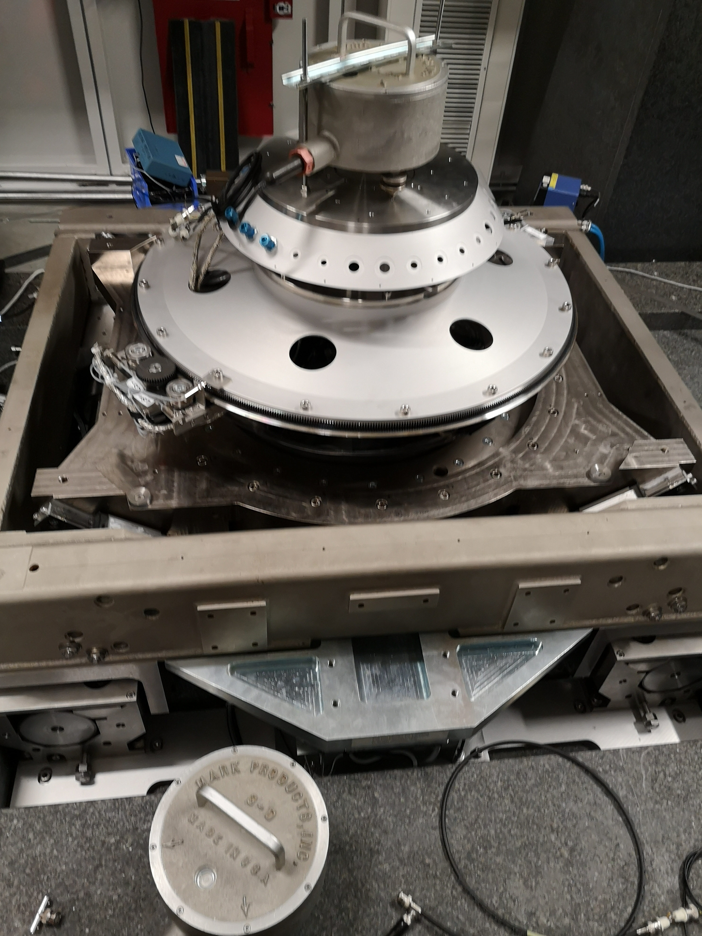
The North of the Geophones corresponds to the +Y direction and the East of the Geophones to the +X direction (see figure fig:experimental_setup_picture).
The spindle and slip-ring are turned ON. The Hexapod and the tilt-stage are OFF.
Goal ignore
Goal:
- Determine the disturbances induced by the translation stage in the Z and X directions when scanning along the Y direction
Measurements ignore
Measurements: Three measurements are done:
| Measurement File | Description |
|---|---|
mat/data_040.mat |
Z direction |
mat/data_041.mat |
E direction |
mat/data_042.mat |
E direction without any motion (Ty OFF) |
Each of the measurement mat file contains one data array with 3 columns:
| Column number | Description |
|---|---|
| 1 | Geophone - Marble |
| 2 | Geophone - Sample |
| 3 | Time |
Measurement Analysis
<<sec:disturbance_ty>>
ZIP file containing the data and matlab files ignore
All the files (data and Matlab scripts) are accessible here.
Load data
  z_ty = load('mat/data_040.mat', 'data'); z_ty = z_ty.data;
  e_ty = load('mat/data_041.mat', 'data'); e_ty = e_ty.data;
  e_of = load('mat/data_042.mat', 'data'); e_of = e_of.data;
Voltage to Velocity
We convert the measured voltage to velocity using the function voltageToVelocityL22 (accessible here).
  gain = 40; % [dB]

  z_ty(:, 1) = voltageToVelocityL22(z_ty(:, 1), z_ty(:, 3), gain);
  e_ty(:, 1) = voltageToVelocityL22(e_ty(:, 1), e_ty(:, 3), gain);
  e_of(:, 1) = voltageToVelocityL22(e_of(:, 1), e_of(:, 3), gain);

  z_ty(:, 2) = voltageToVelocityL22(z_ty(:, 2), z_ty(:, 3), gain);
  e_ty(:, 2) = voltageToVelocityL22(e_ty(:, 2), e_ty(:, 3), gain);
  e_of(:, 2) = voltageToVelocityL22(e_of(:, 2), e_of(:, 3), gain);
Time domain plots
We plot the measured velocity of the marble and sample in the vertical direction (figure fig:ty_z_time) and in the X direction (figure fig:ty_e_time).
We also integrate the relative velocity to obtain the relative displacement (figure fig:x_relative_disp in the X direction and figure fig:z_relative_disp in the Z direction).
  figure;
  hold on;
  plot(z_ty(:, 3), z_ty(:, 1), 'DisplayName', 'Marble - Z');
  plot(z_ty(:, 3), z_ty(:, 2), 'DisplayName', 'Sample - Z');
  hold off;
  xlabel('Time [s]'); ylabel('Velocity [m/s]');
  xlim([0, 2]);
legend('Location', 'northeast'); <<plt-matlab>>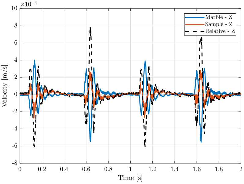
  figure;
  hold on;
  plot(e_ty(:, 3), e_ty(:, 1), 'DisplayName', 'Marble - X');
  plot(e_ty(:, 3), e_ty(:, 2), 'DisplayName', 'Sample - X');
  hold off;
  xlabel('Time [s]'); ylabel('Velocity [m/s]');
  xlim([0, 2]);
legend('Location', 'northeast'); <<plt-matlab>>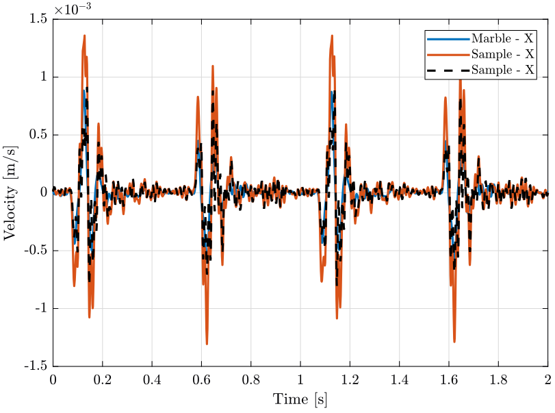
  figure;
  plot(e_ty(:, 3), 1e6*lsim(1/s, e_ty(:, 2)-e_ty(:, 1), e_ty(:, 3)));
  xlabel('Time [s]'); ylabel('X Relative Displacement [$\mu m$]');
xlim([0, 2]); <<plt-matlab>>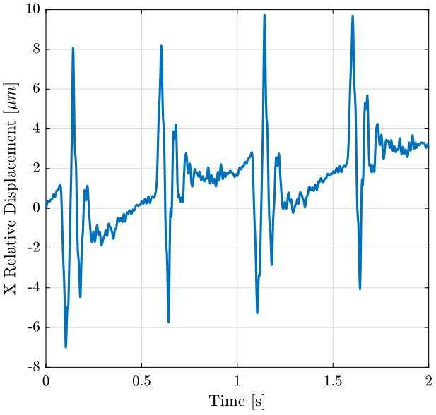
  figure;
  plot(z_ty(:, 3), 1e6*lsim(1/s, z_ty(:, 2)-z_ty(:, 1), z_ty(:, 3)));
  xlabel('Time [s]'); ylabel('Z Relative Displacement [$\mu m$]');
xlim([0, 2]); <<plt-matlab>>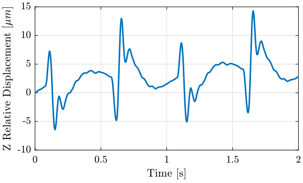
Frequency Domain analysis
We get the typical ground velocity to compare with the velocities measured.
[pxx_gm, f_gm] = getPSDGroundVelocity();We first compute some parameters that will be used for the PSD computation.
  dt = z_ty(2, 3)-z_ty(1, 3);

  Fs = 1/dt; % [Hz]

  win = hanning(ceil(10*Fs));
Then we compute the Power Spectral Density using pwelch function.
First for the geophone located on the marble
  [pxz_ty_m, f] = pwelch(z_ty(:, 1), win, [], [], Fs);
  [pxe_ty_m, ~] = pwelch(e_ty(:, 1), win, [], [], Fs);
  [pxe_of_m, ~] = pwelch(e_of(:, 1), win, [], [], Fs);
And for the geophone located at the sample position.
  [pxz_ty_s, ~] = pwelch(z_ty(:, 2), win, [], [], Fs);
  [pxe_ty_s, ~] = pwelch(e_ty(:, 2), win, [], [], Fs);
  [pxe_of_s, ~] = pwelch(e_of(:, 2), win, [], [], Fs);
And finally for the relative velocity between the sample and the marble.
  [pxz_ty_r, ~] = pwelch(z_ty(:, 2)-z_ty(:, 1), win, [], [], Fs);
  [pxe_ty_r, ~] = pwelch(e_ty(:, 2)-e_ty(:, 1), win, [], [], Fs);
  [pxe_of_r, ~] = pwelch(e_of(:, 2)-e_of(:, 1), win, [], [], Fs);
And we plot the ASD of the measured velocities:
- figure fig:asd_east_marble compares the marble velocity in the east direction when scanning and when Ty is OFF
- figure fig:asd_east_sample compares the sample velocity in the east direction when scanning and when Ty is OFF
- figure fig:asd_z_direction shows the marble and sample velocities in the Z direction when scanning with the translation stage
- figure fig:asd_e_relative shows the relative velocity of the sample with respect to the granite in the X direction when the translation stage is OFF and when it is scanning at 1Hz
  figure;
  hold on;
  plot(f, sqrt(pxe_ty_m), 'DisplayName', 'Ty 1Hz - Marble - X');
  plot(f, sqrt(pxe_of_m), 'DisplayName', 'Ty OFF - Marble - X');
  plot(f_gm, sqrt(pxx_gm), 'k--', 'DisplayName', 'Ground Motion');
  hold off;
  set(gca, 'xscale', 'log');
  set(gca, 'yscale', 'log');
  xlabel('Frequency [Hz]'); ylabel('ASD of the measured velocity $\left[\frac{m/s}{\sqrt{Hz}}\right]$')
  legend('Location', 'northwest');
xlim([0.1, 500]); <<plt-matlab>>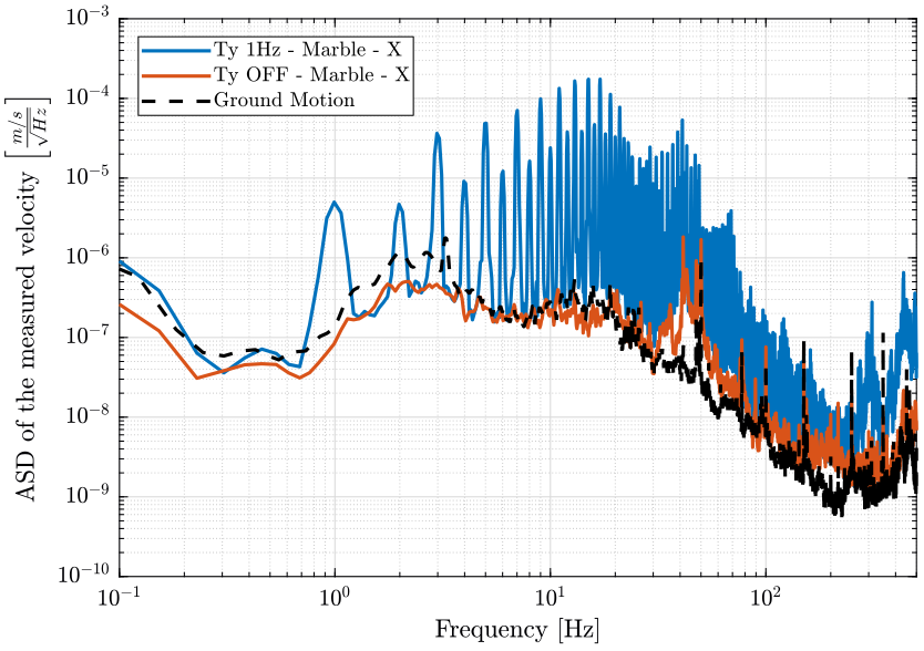
  figure;
  hold on;
  plot(f, sqrt(pxe_ty_s), 'DisplayName', 'Ty 1Hz - Sample - X');
  plot(f, sqrt(pxe_of_s), 'DisplayName', 'Ty OFF - Sample - X');
  plot(f_gm, sqrt(pxx_gm), 'k--', 'DisplayName', 'Ground Motion');
  hold off;
  set(gca, 'xscale', 'log');
  set(gca, 'yscale', 'log');
  xlabel('Frequency [Hz]'); ylabel('ASD of the measured velocity $\left[\frac{m/s}{\sqrt{Hz}}\right]$')
  legend('Location', 'northwest');
xlim([0.1, 500]); <<plt-matlab>>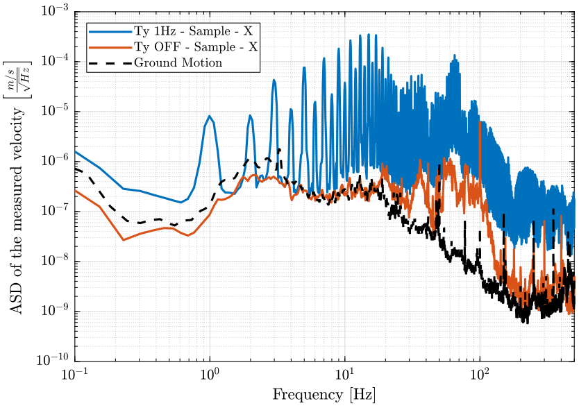
  figure;
  hold on;
  plot(f, sqrt(pxz_ty_m), 'DisplayName', 'Ty 1Hz - Marble - Z');
  plot(f, sqrt(pxz_ty_s), 'DisplayName', 'Ty 1Hz - Sample - Z');
  plot(f_gm, sqrt(pxx_gm), 'k--', 'DisplayName', 'Ground Motion');
  hold off;
  set(gca, 'xscale', 'log');
  set(gca, 'yscale', 'log');
  xlabel('Frequency [Hz]'); ylabel('ASD of the measured velocity $\left[\frac{m/s}{\sqrt{Hz}}\right]$')
  legend('Location', 'northwest');
xlim([0.1, 500]); <<plt-matlab>>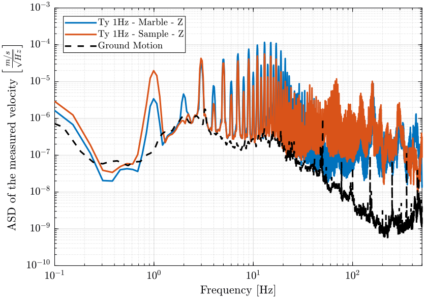
  figure;
  hold on;
  plot(f, sqrt(pxe_of_r), 'DisplayName', 'Ty OFF - Relative - E');
  plot(f, sqrt(pxe_ty_r), 'DisplayName', 'Ty 1Hz - Relative - E');
  hold off;
  set(gca, 'xscale', 'log');
  set(gca, 'yscale', 'log');
  xlabel('Frequency [Hz]'); ylabel('ASD of the measured velocity $\left[\frac{m/s}{\sqrt{Hz}}\right]$')
  legend('Location', 'northwest');
xlim([0.1, 500]); <<plt-matlab>>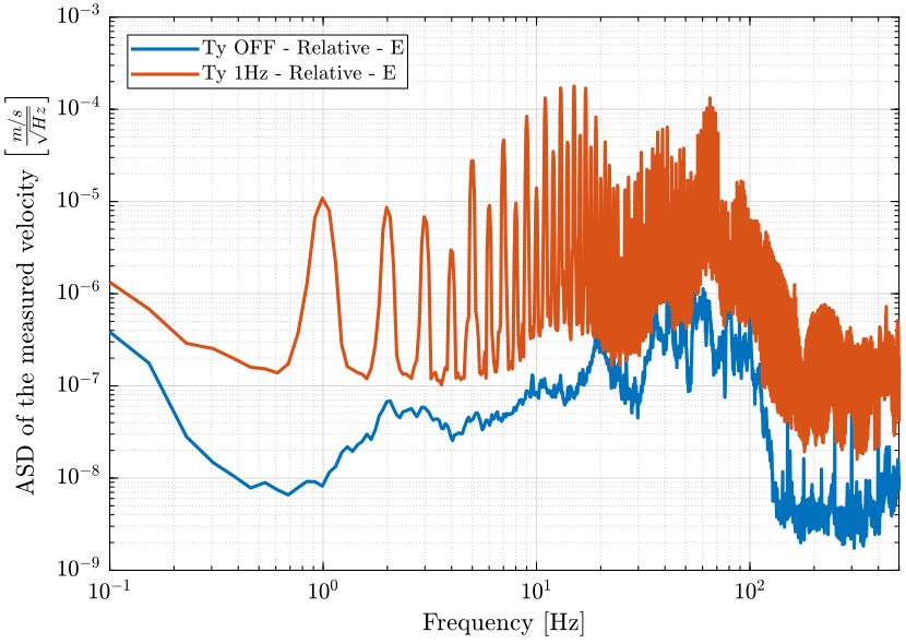
Transfer function from marble motion in the East direction to sample motion in the East direction
Let's compute the transfer function for the marble velocity in the east direction to the sample velocity in the east direction.
We first plot the time domain motions when every stage is off (figure fig:east_marble_sample).
  figure;
  hold on;
  plot(e_of(:, 3), e_of(:, 2), 'DisplayName', 'Sample - X');
  plot(e_of(:, 3), e_of(:, 1), 'DisplayName', 'Marble - X');
  hold off;
  xlabel('Time [s]'); ylabel('Velocity [m/s]');
  xlim([0, 100]);
legend('Location', 'southwest'); <<plt-matlab>>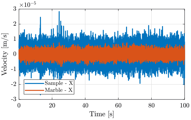
We then compute the transfer function using tfestimate.
  dt = e_of(2, 3)-e_of(1, 3);
  Fs = 1/dt; % [Hz]
  win = hanning(ceil(10*Fs));

  [T, f] = tfestimate(e_of(:, 1), e_of(:, 2), win, [], [], Fs);
The result is shown on figure fig:tf_east_marble_sample.
<<plt-matlab>>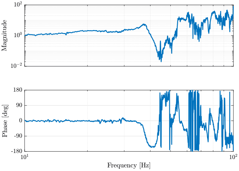
Position of the translation stage and Current
The position of the translation and current flowing in its actuator are measured using the elmo software and saved as an csv file.
Data pre-processing
Let's look at at the start of the csv file.
sed -n 1,30p mat/sin_elmo.csv | nl -ba - 1 Elmo txt chart ver 2.0
2
3 [File Properties]
4 Creation Time,2019-05-13 05:11:45
5 Last Updated,2019-05-13 05:11:45
6 Resolution,0.001
7 Sampling Time,5E-05
8 Recording Time,5.461
9
10 [Chart Properties]
11 No.,Name,X Linear,X No.
12 1,Chart #1,True,0
13 2,Chart #2,True,0
14
15 [Chart Data]
16 Display No.,X No.,Y No.,X Unit,Y Unit,Color,Style,Width
17 1,1,2,sec,N/A,ff0000ff,Solid,TwoPoint
18 2,1,3,sec,N/A,ff0000ff,Solid,TwoPoint
19 2,1,4,sec,N/A,ff007f00,Solid,TwoPoint
20
21 [Signal Names]
22 1,Time (sec)
23 2,Position [cnt]
24 3,Current Command [A]
25 4,Total Current Command [A]
26
27 [Signals Data Group 1]
28 1,2,3,4,
29 0,1110769,-0.320872406596209,-0.320872406596209,
30 0.001,1108743,-0.319658428261391,-0.319658428261391,
The real data starts at line 29.
We then load this cvs file starting at line 29.
data = csvread("mat/sin_elmo.csv", 29, 0);Time domain data
We plot the position of the translation stage measured by the encoders. There is 200000 encoder count for each mm, we then divide by 200000 to obtain mm. The result is shown on figure fig:ty_position_time.
  figure;
  hold on;
  plot(data(:, 1), data(:, 2)/200000);
  hold off;
  xlim([0, 5]);
xlabel('Time [s]'); ylabel('Position [mm]'); <<plt-matlab>>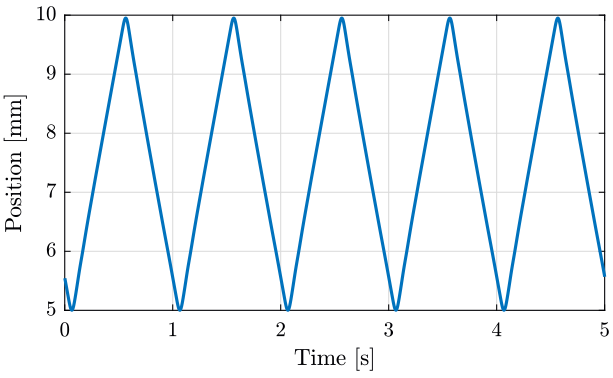
<<plt-matlab>>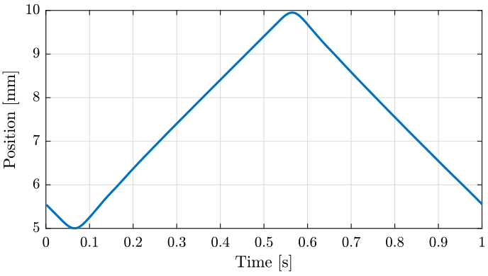
We also plot the current as function of the time on figure fig:current_time.
  figure;
  hold on;
  plot(data(:, 1), data(:, 3));
  hold off;
  xlim([0, 5]); ylim([-10, 10]);
xlabel('Time [s]'); ylabel('Current [A]'); <<plt-matlab>>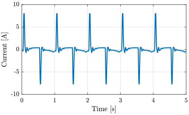
<<plt-matlab>>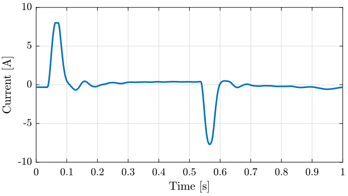
Conclusion
- The acquisition is done using the Speedgoat as well as using ELMO. The two acquisition are not synchronize
- The value of the translation stage encoder can also be read with the speedgoat, this could permit to synchronize the measurements