29 KiB
- Effect of all the control systems on the Sample vibrations
- Effect of all the control systems on the Sample vibrations - One stage at a time
- Effect of the Symetrie Driver
#+TITLE:Effect on the control system of each stages on the vibration of the station
This file is organized as follow:
-
Section sec:effect_control_all:
- One geophone on the marble and one at the sample location
- Each stage is turned on one by one
-
Section sec:effect_control_one:
- One geophone on the marble and one at the sample location
- Each stage is turned on one at a time
-
Section sec:effect_symetrie_driver:
- We check if the Symetrie driver induces some vibrations when placed on the marble
Effect of all the control systems on the Sample vibrations
<<sec:effect_control_all>>
ZIP file containing the data and matlab files ignore
All the files (data and Matlab scripts) are accessible here.
Experimental Setup
We here measure the signals of two L22 geophones:
- One is located on top of the Sample platform
- One is located on the marble
The signals are amplified with voltage amplifiers with the following settings:
- gain of 60dB
- AC/DC option set on AC
- Low pass filter set at 1kHz
The signal from the top geophone does not go trought the slip-ring.
First, all the control systems are turned ON, then, they are turned one by one. Each measurement are done during 50s.
| Ty | Ry | Slip Ring | Spindle | Hexapod | Meas. file |
|---|---|---|---|---|---|
| ON | ON | ON | ON | ON | meas_003.mat |
| OFF | ON | ON | ON | ON | meas_004.mat |
| OFF | OFF | ON | ON | ON | meas_005.mat |
| OFF | OFF | OFF | ON | ON | meas_006.mat |
| OFF | OFF | OFF | OFF | ON | meas_007.mat |
| OFF | OFF | OFF | OFF | OFF | meas_008.mat |
Each of the mat file contains one array data with 3 columns:
| Column number | Description |
|---|---|
| 1 | Geophone - Marble |
| 2 | Geophone - Sample |
| 3 | Time |
Load data
We load the data of the z axis of two geophones.
  d3 = load('mat/data_003.mat', 'data'); d3 = d3.data;
  d4 = load('mat/data_004.mat', 'data'); d4 = d4.data;
  d5 = load('mat/data_005.mat', 'data'); d5 = d5.data;
  d6 = load('mat/data_006.mat', 'data'); d6 = d6.data;
  d7 = load('mat/data_007.mat', 'data'); d7 = d7.data;
  d8 = load('mat/data_008.mat', 'data'); d8 = d8.data;
Analysis - Time Domain
First, we can look at the time domain data and compare all the measurements:
- comparison for the geophone at the sample location (figure fig:time_domain_sample)
- comparison for the geophone on the granite (figure fig:time_domain_marble)
  figure;
  hold on;
  plot(d3(:, 3), d3(:, 2), 'DisplayName', 'Hexa, Rz, SR, Ry, Ty');
  plot(d4(:, 3), d4(:, 2), 'DisplayName', 'Hexa, Rz, SR, Ry');
  plot(d5(:, 3), d5(:, 2), 'DisplayName', 'Hexa, Rz, SR');
  plot(d6(:, 3), d6(:, 2), 'DisplayName', 'Hexa, Rz');
  plot(d7(:, 3), d7(:, 2), 'DisplayName', 'Hexa');
  plot(d8(:, 3), d8(:, 2), 'DisplayName', 'All OFF');
  hold off;
  xlabel('Time [s]'); ylabel('Voltage [V]');
  xlim([0, 50]);
legend('Location', 'bestoutside'); <<plt-matlab>>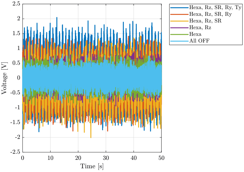
  figure;
  hold on;
  plot(d3(:, 3), d3(:, 1), 'DisplayName', 'Hexa, Rz, SR, Ry, Ty');
  plot(d4(:, 3), d4(:, 1), 'DisplayName', 'Hexa, Rz, SR, Ry');
  plot(d5(:, 3), d5(:, 1), 'DisplayName', 'Hexa, Rz, SR');
  plot(d6(:, 3), d6(:, 1), 'DisplayName', 'Hexa, Rz');
  plot(d7(:, 3), d7(:, 1), 'DisplayName', 'Hexa');
  plot(d8(:, 3), d8(:, 1), 'DisplayName', 'All OFF');
  hold off;
  xlabel('Time [s]'); ylabel('Voltage [V]');
  xlim([0, 50]);
legend('Location', 'bestoutside'); <<plt-matlab>>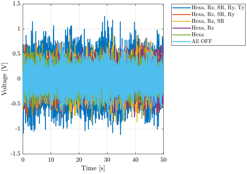
Analysis - Frequency Domain
  dt = d3(2, 3) - d3(1, 3);

  Fs = 1/dt;
  win = hanning(ceil(10*Fs));
Vibrations at the sample location
First, we compute the Power Spectral Density of the signals coming from the Geophone located at the sample location.
  [px3, f] = pwelch(d3(:, 2), win, [], [], Fs);
  [px4, ~] = pwelch(d4(:, 2), win, [], [], Fs);
  [px5, ~] = pwelch(d5(:, 2), win, [], [], Fs);
  [px6, ~] = pwelch(d6(:, 2), win, [], [], Fs);
  [px7, ~] = pwelch(d7(:, 2), win, [], [], Fs);
  [px8, ~] = pwelch(d8(:, 2), win, [], [], Fs);
And we compare all the signals (figures fig:psd_sample_comp and fig:psd_sample_comp_high_freq).
  figure;
  hold on;
  plot(f, sqrt(px3), 'DisplayName', 'Hexa, Rz, SR, Ry, Ty');
  plot(f, sqrt(px4), 'DisplayName', 'Hexa, Rz, SR, Ry');
  plot(f, sqrt(px5), 'DisplayName', 'Hexa, Rz, SR');
  plot(f, sqrt(px6), 'DisplayName', 'Hexa, Rz');
  plot(f, sqrt(px7), 'DisplayName', 'Hexa');
  plot(f, sqrt(px8), 'DisplayName', 'All OFF');
  plot(fgm, sqrt(pxxgm), '-k', 'DisplayName', 'Ground Velocity');
  hold off;
  set(gca, 'xscale', 'log');
  set(gca, 'yscale', 'log');
  xlabel('Frequency [Hz]'); ylabel('Amplitude Spectral Density $\left[\frac{V}{\sqrt{Hz}}\right]$')
  xlim([0.1, 500]);
legend('Location', 'southwest'); <<plt-matlab>>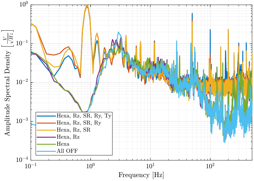
<<plt-matlab>>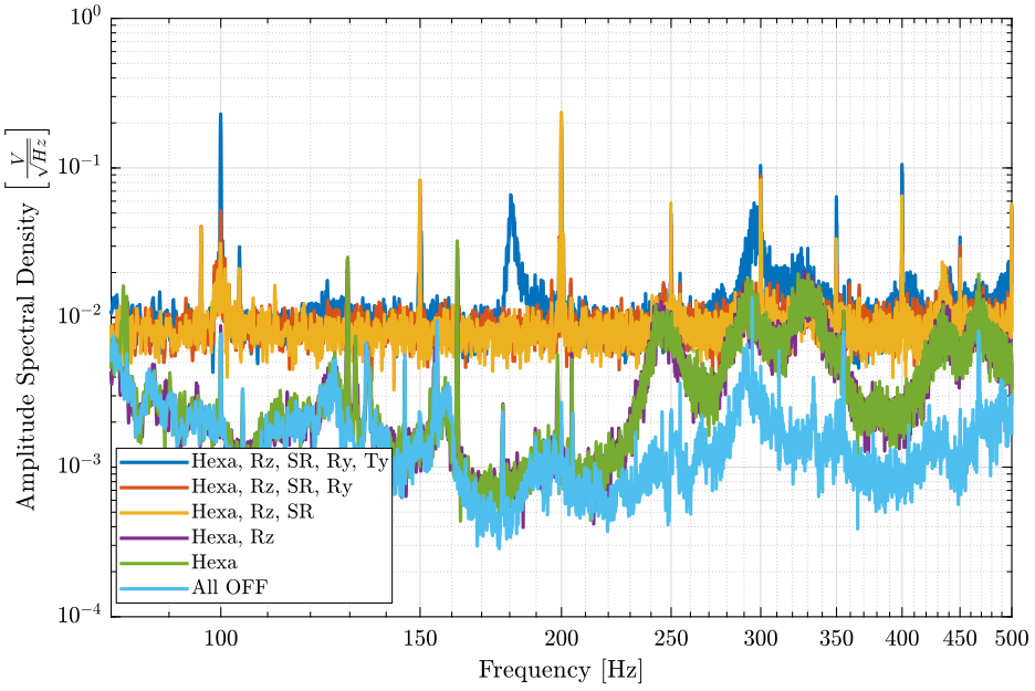
Vibrations on the marble
Now we plot the same curves for the geophone located on the marble.
  [px3, f] = pwelch(d3(:, 1), win, [], [], Fs);
  [px4, ~] = pwelch(d4(:, 1), win, [], [], Fs);
  [px5, ~] = pwelch(d5(:, 1), win, [], [], Fs);
  [px6, ~] = pwelch(d6(:, 1), win, [], [], Fs);
  [px7, ~] = pwelch(d7(:, 1), win, [], [], Fs);
  [px8, ~] = pwelch(d8(:, 1), win, [], [], Fs);
And we compare the Amplitude Spectral Densities (figures fig:psd_marble_comp and fig:psd_marble_comp_high_freq)
  figure;
  hold on;
  plot(f, sqrt(px3), 'DisplayName', 'Hexa, Rz, SR, Ry, Ty');
  plot(f, sqrt(px4), 'DisplayName', 'Hexa, Rz, SR, Ry');
  plot(f, sqrt(px5), 'DisplayName', 'Hexa, Rz, SR');
  plot(f, sqrt(px6), 'DisplayName', 'Hexa, Rz');
  plot(f, sqrt(px7), 'DisplayName', 'Hexa');
  plot(f, sqrt(px8), 'DisplayName', 'All OFF');
  plot(fgm, sqrt(pxxgm), '-k', 'DisplayName', 'Ground Velocity');
  hold off;
  set(gca, 'xscale', 'log');
  set(gca, 'yscale', 'log');
  xlabel('Frequency [Hz]'); ylabel('Amplitude Spectral Density $\left[\frac{V}{\sqrt{Hz}}\right]$')
  xlim([0.1, 500]);
legend('Location', 'northeast'); <<plt-matlab>>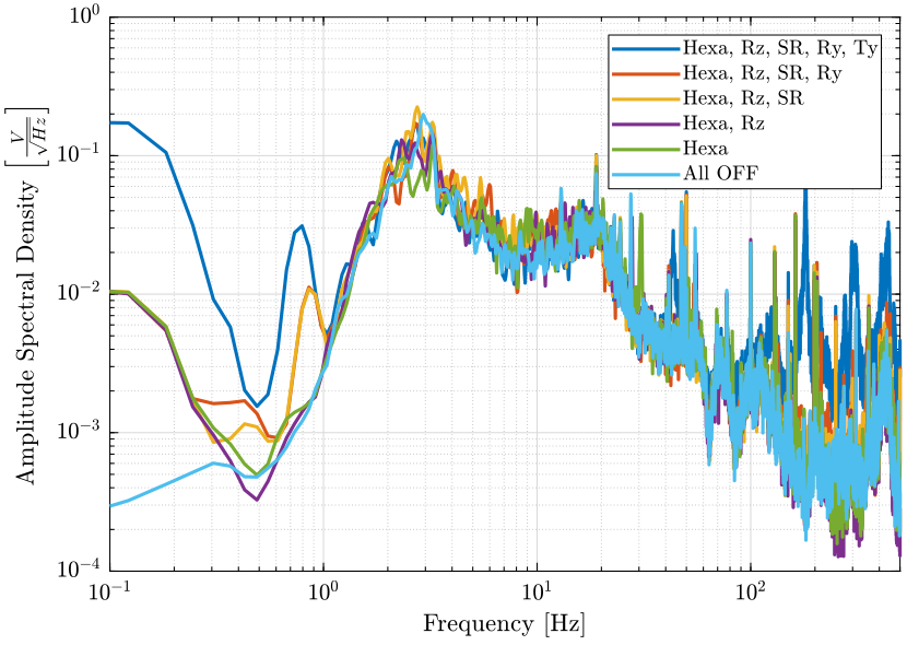
<<plt-matlab>>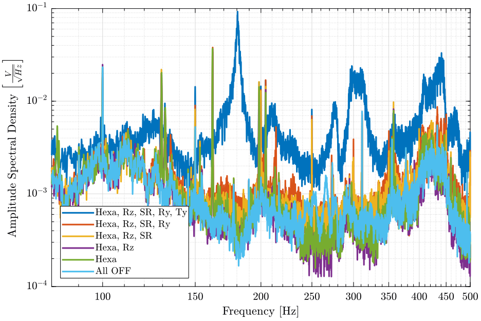
Conclusion
- The control system of the Ty stage induces a lot of vibrations of the marble above 100Hz
- The hexapod control system add vibrations of the sample only above 200Hz
- When the Slip-Ring is ON, white noise appears at high frequencies. This is studied here
Effect of all the control systems on the Sample vibrations - One stage at a time
<<sec:effect_control_one>>
ZIP file containing the data and matlab files ignore
All the files (data and Matlab scripts) are accessible here.
Experimental Setup
We here measure the signals of two geophones:
- One is located on top of the Sample platform
- One is located on the marble
The signal from the top geophone does go trought the slip-ring.
All the control systems are turned OFF, then, they are turned on one at a time.
Each measurement are done during 100s.
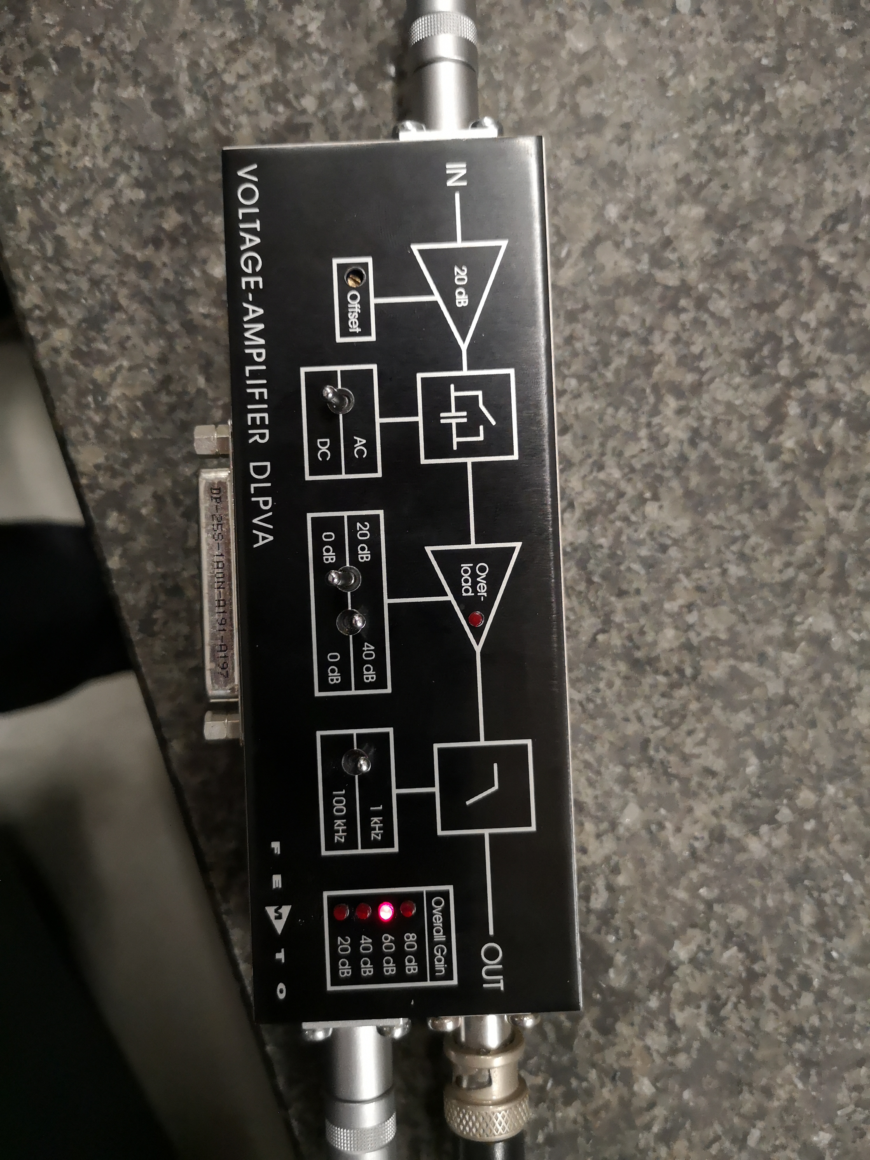
The settings of the voltage amplifier are shown on figure fig:amplifier_settings:
- gain of 60dB
- AC/DC option set on DC
- Low pass filter set at 1kHz
A first order low pass filter with a cut-off frequency of 1kHz is added before the voltage amplifier.
| Ty | Ry | Slip Ring | Spindle | Hexapod | Meas. file |
|---|---|---|---|---|---|
| OFF | OFF | OFF | OFF | OFF | meas_013.mat |
| ON | OFF | OFF | OFF | OFF | meas_014.mat |
| OFF | ON | OFF | OFF | OFF | meas_015.mat |
| OFF | OFF | ON | OFF | OFF | meas_016.mat |
| OFF | OFF | OFF | ON | OFF | meas_017.mat |
| OFF | OFF | OFF | OFF | ON | meas_018.mat |
Each of the mat file contains one array data with 3 columns:
| Column number | Description |
|---|---|
| 1 | Geophone - Marble |
| 2 | Geophone - Sample |
| 3 | Time |
Load data
We load the data of the z axis of two geophones.
  d_of = load('mat/data_013.mat', 'data'); d_of = d_of.data;
  d_ty = load('mat/data_014.mat', 'data'); d_ty = d_ty.data;
  d_ry = load('mat/data_015.mat', 'data'); d_ry = d_ry.data;
  d_sr = load('mat/data_016.mat', 'data'); d_sr = d_sr.data;
  d_rz = load('mat/data_017.mat', 'data'); d_rz = d_rz.data;
  d_he = load('mat/data_018.mat', 'data'); d_he = d_he.data;
Voltage to Velocity
We convert the measured voltage to velocity using the function voltageToVelocityL22 (accessible here).
  gain = 60; % [dB]

  d_of(:, 1) = voltageToVelocityL22(d_of(:, 1), d_of(:, 3), gain);
  d_ty(:, 1) = voltageToVelocityL22(d_ty(:, 1), d_ty(:, 3), gain);
  d_ry(:, 1) = voltageToVelocityL22(d_ry(:, 1), d_ry(:, 3), gain);
  d_sr(:, 1) = voltageToVelocityL22(d_sr(:, 1), d_sr(:, 3), gain);
  d_rz(:, 1) = voltageToVelocityL22(d_rz(:, 1), d_rz(:, 3), gain);
  d_he(:, 1) = voltageToVelocityL22(d_he(:, 1), d_he(:, 3), gain);

  d_of(:, 2) = voltageToVelocityL22(d_of(:, 2), d_of(:, 3), gain);
  d_ty(:, 2) = voltageToVelocityL22(d_ty(:, 2), d_ty(:, 3), gain);
  d_ry(:, 2) = voltageToVelocityL22(d_ry(:, 2), d_ry(:, 3), gain);
  d_sr(:, 2) = voltageToVelocityL22(d_sr(:, 2), d_sr(:, 3), gain);
  d_rz(:, 2) = voltageToVelocityL22(d_rz(:, 2), d_rz(:, 3), gain);
  d_he(:, 2) = voltageToVelocityL22(d_he(:, 2), d_he(:, 3), gain);
Analysis - Time Domain
First, we can look at the time domain data and compare all the measurements:
- comparison for the geophone at the sample location (figure fig:time_domain_sample_lpf)
- comparison for the geophone on the granite (figure fig:time_domain_marble_lpf)
- relative displacement of the sample with respect to the marble (figure fig:time_domain_marble_lpf)
  figure;
  hold on;
  plot(d_of(:, 3), d_of(:, 2), 'DisplayName', 'All OFF');
  plot(d_ty(:, 3), d_ty(:, 2), 'DisplayName', 'Ty ON');
  plot(d_ry(:, 3), d_ry(:, 2), 'DisplayName', 'Ry ON');
  plot(d_sr(:, 3), d_sr(:, 2), 'DisplayName', 'S-R ON');
  plot(d_rz(:, 3), d_rz(:, 2), 'DisplayName', 'Rz ON');
  plot(d_he(:, 3), d_he(:, 2), 'DisplayName', 'Hexa ON');
  hold off;
  xlabel('Time [s]'); ylabel('Velocity [m/s]');
  xlim([0, 50]);
legend('Location', 'bestoutside'); <<plt-matlab>>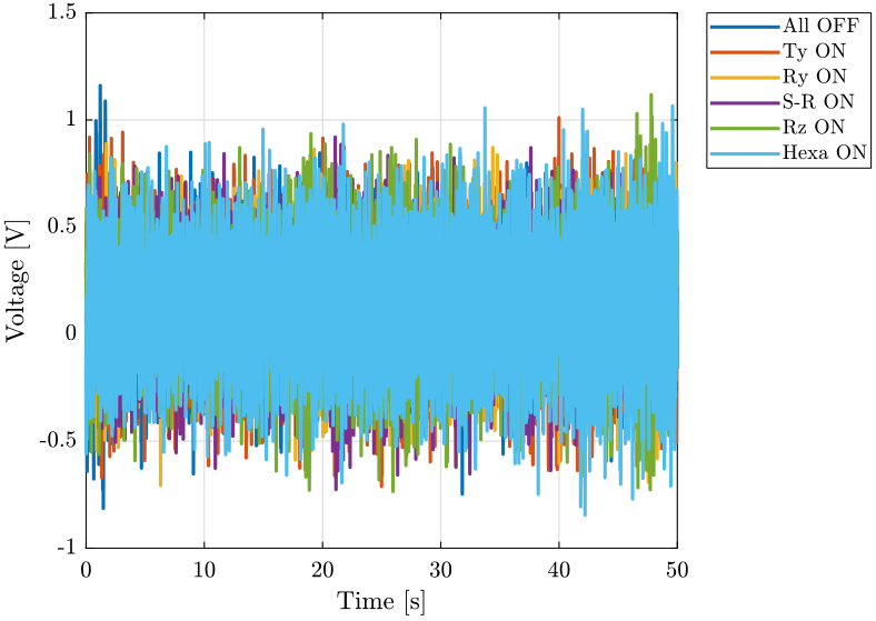
  figure;
  hold on;
  plot(d_of(:, 3), d_of(:, 1), 'DisplayName', 'All OFF');
  plot(d_ty(:, 3), d_ty(:, 1), 'DisplayName', 'Ty ON');
  plot(d_ry(:, 3), d_ry(:, 1), 'DisplayName', 'Ry ON');
  plot(d_sr(:, 3), d_sr(:, 1), 'DisplayName', 'S-R ON');
  plot(d_rz(:, 3), d_rz(:, 1), 'DisplayName', 'Rz ON');
  plot(d_he(:, 3), d_he(:, 1), 'DisplayName', 'Hexa ON');
  hold off;
  xlabel('Time [s]'); ylabel('Velocity [m/s]');
  xlim([0, 50]);
legend('Location', 'bestoutside'); <<plt-matlab>>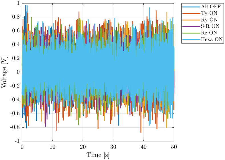
  figure;
  hold on;
  plot(d_of(:, 3), 1e6*lsim(1/(1+s/(2*pi*0.5)), d_of(:, 2)-d_of(:, 1), d_of(:, 3)), 'DisplayName', 'All OFF');
  plot(d_ty(:, 3), 1e6*lsim(1/(1+s/(2*pi*0.5)), d_ty(:, 2)-d_ty(:, 1), d_ty(:, 3)), 'DisplayName', 'Ty ON');
  plot(d_ry(:, 3), 1e6*lsim(1/(1+s/(2*pi*0.5)), d_ry(:, 2)-d_ry(:, 1), d_ry(:, 3)), 'DisplayName', 'Ry ON');
  plot(d_sr(:, 3), 1e6*lsim(1/(1+s/(2*pi*0.5)), d_sr(:, 2)-d_sr(:, 1), d_sr(:, 3)), 'DisplayName', 'S-R ON');
  plot(d_rz(:, 3), 1e6*lsim(1/(1+s/(2*pi*0.5)), d_rz(:, 2)-d_rz(:, 1), d_rz(:, 3)), 'DisplayName', 'Rz ON');
  plot(d_he(:, 3), 1e6*lsim(1/(1+s/(2*pi*0.5)), d_he(:, 2)-d_he(:, 1), d_he(:, 3)), 'DisplayName', 'Hexa ON');
  hold off;
  xlabel('Time [s]'); ylabel('Relative Displacement [$\mu m$]');
  xlim([0, 50]);
legend('Location', 'bestoutside'); <<plt-matlab>>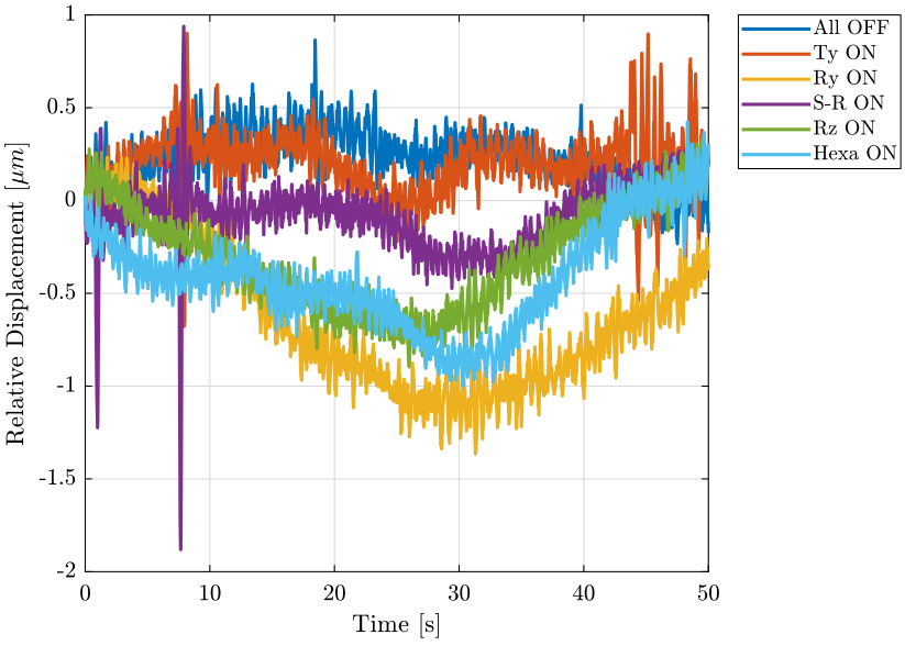
Analysis - Frequency Domain
  dt = d_of(2, 3) - d_of(1, 3);

  Fs = 1/dt;
  win = hanning(ceil(10*Fs));
Vibrations at the sample location
First, we compute the Power Spectral Density of the signals coming from the Geophone located at the sample location.
  [px_of, f] = pwelch(d_of(:, 2), win, [], [], Fs);
  [px_ty, ~] = pwelch(d_ty(:, 2), win, [], [], Fs);
  [px_ry, ~] = pwelch(d_ry(:, 2), win, [], [], Fs);
  [px_sr, ~] = pwelch(d_sr(:, 2), win, [], [], Fs);
  [px_rz, ~] = pwelch(d_rz(:, 2), win, [], [], Fs);
  [px_he, ~] = pwelch(d_he(:, 2), win, [], [], Fs);
And we compare all the signals (figures fig:psd_sample_comp_lpf and fig:psd_sample_comp_high_freq_lpf).
  figure;
  hold on;
  plot(f, sqrt(px_of), 'DisplayName', 'All OFF');
  plot(f, sqrt(px_ty), 'DisplayName', 'Ty ON');
  plot(f, sqrt(px_ry), 'DisplayName', 'Ry ON');
  plot(f, sqrt(px_sr), 'DisplayName', 'S-R ON');
  plot(f, sqrt(px_rz), 'DisplayName', 'Rz ON');
  plot(f, sqrt(px_he), 'DisplayName', 'Hexa ON');
  hold off;
  set(gca, 'xscale', 'log');
  set(gca, 'yscale', 'log');
  xlabel('Frequency [Hz]'); ylabel('Amplitude Spectral Density $\left[\frac{m/s}{\sqrt{Hz}}\right]$')
  xlim([0.1, 500]);
legend('Location', 'southwest'); <<plt-matlab>>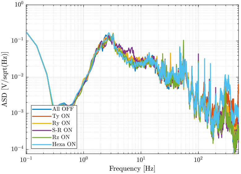
<<plt-matlab>>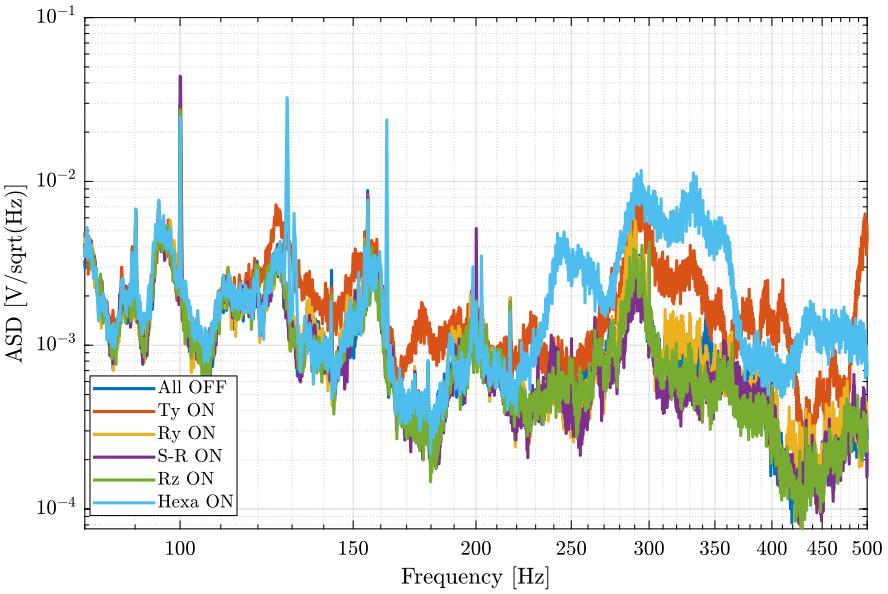
Vibrations on the marble
Now we plot the same curves for the geophone located on the marble.
  [px_of, f] = pwelch(d_of(:, 1), win, [], [], Fs);
  [px_ty, ~] = pwelch(d_ty(:, 1), win, [], [], Fs);
  [px_ry, ~] = pwelch(d_ry(:, 1), win, [], [], Fs);
  [px_sr, ~] = pwelch(d_sr(:, 1), win, [], [], Fs);
  [px_rz, ~] = pwelch(d_rz(:, 1), win, [], [], Fs);
  [px_he, ~] = pwelch(d_he(:, 1), win, [], [], Fs);
And we compare the Amplitude Spectral Densities (figures fig:psd_marble_comp_lpf and fig:psd_marble_comp_lpf_high_freq)
  figure;
  hold on;
  plot(f, sqrt(px_of), 'DisplayName', 'All OFF');
  plot(f, sqrt(px_ty), 'DisplayName', 'Ty ON');
  plot(f, sqrt(px_ry), 'DisplayName', 'Ry ON');
  plot(f, sqrt(px_sr), 'DisplayName', 'S-R ON');
  plot(f, sqrt(px_rz), 'DisplayName', 'Rz ON');
  plot(f, sqrt(px_he), 'DisplayName', 'Hexa ON');
  hold off;
  set(gca, 'xscale', 'log');
  set(gca, 'yscale', 'log');
  xlabel('Frequency [Hz]'); ylabel('Amplitude Spectral Density $\left[\frac{m/s}{\sqrt{Hz}}\right]$')
  xlim([0.1, 500]);
legend('Location', 'northeast'); <<plt-matlab>>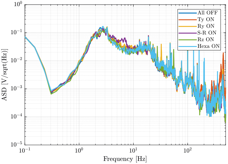
<<plt-matlab>>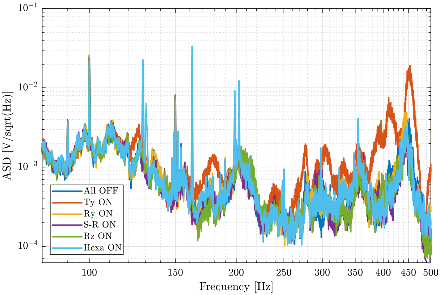
Conclusion
- The Ty stage induces vibrations of the marble and at the sample location above 100Hz
- The hexapod stage induces vibrations at the sample position above 220Hz
Effect of the Symetrie Driver
<<sec:effect_symetrie_driver>>
ZIP file containing the data and matlab files ignore
All the files (data and Matlab scripts) are accessible here.
Experimental Setup
We here measure the signals of two geophones:
- One is located on top of the Sample platform
- One is located on the marble
The signal from the top geophone does go trought the slip-ring.
All the control systems are turned OFF except the Hexapod one.
Each measurement are done during 100s.
The settings of the voltage amplifier are:
- gain of 60dB
- AC/DC option set on DC
- Low pass filter set at 1kHz
A first order low pass filter with a cut-off frequency of 1kHz is added before the voltage amplifier.
The measurements are:
meas_018.mat: Hexapod's driver on the granitemeas_019.mat: Hexapod's driver on the ground
Each of the mat file contains one array data with 3 columns:
| Column number | Description |
|---|---|
| 1 | Geophone - Marble |
| 2 | Geophone - Sample |
| 3 | Time |
Load data
We load the data of the z axis of two geophones.
  d_18 = load('mat/data_018.mat', 'data'); d_18 = d_18.data;
  d_19 = load('mat/data_019.mat', 'data'); d_19 = d_19.data;
Analysis - Time Domain
  figure;
  hold on;
  plot(d_19(:, 3), d_19(:, 1), 'DisplayName', 'Driver - Ground');
  plot(d_18(:, 3), d_18(:, 1), 'DisplayName', 'Driver - Granite');
  hold off;
  xlabel('Time [s]'); ylabel('Voltage [V]');
  xlim([0, 50]);
legend('Location', 'bestoutside'); <<plt-matlab>>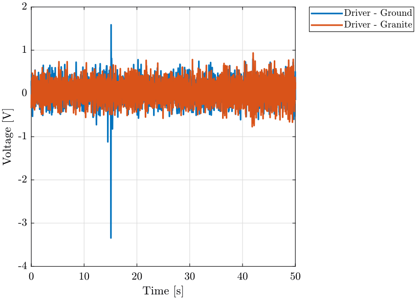
Analysis - Frequency Domain
  dt = d_18(2, 3) - d_18(1, 3);

  Fs = 1/dt;
  win = hanning(ceil(10*Fs));
Vibrations at the sample location
First, we compute the Power Spectral Density of the signals coming from the Geophone located at the sample location.
  [px_18, f] = pwelch(d_18(:, 1), win, [], [], Fs);
[px_19, ~] = pwelch(d_19(:, 1), win, [], [], Fs); figure;
hold on;
plot(f, sqrt(px_19), 'DisplayName', 'Driver - Ground');
plot(f, sqrt(px_18), 'DisplayName', 'Driver - Granite');
hold off;
set(gca, 'xscale', 'log');
set(gca, 'yscale', 'log');
xlabel('Frequency [Hz]'); ylabel('Amplitude Spectral Density $\left[\frac{V}{\sqrt{Hz}}\right]$')
xlim([0.1, 500]);
legend('Location', 'southwest'); <<plt-matlab>>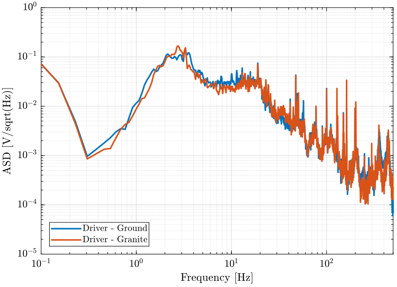
<<plt-matlab>>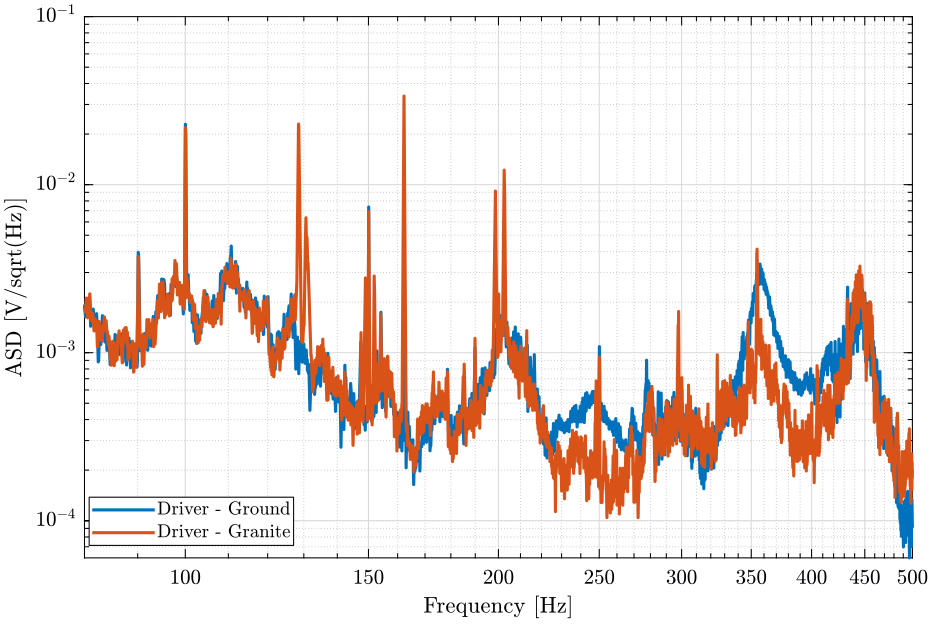
Conclusion
Even tough the Hexapod's driver vibrates quite a lot, it does not generate significant vibrations of the granite when either placed on the granite or on the ground.