19 KiB
Vibrations induced by the Slip-Ring and the Spindle
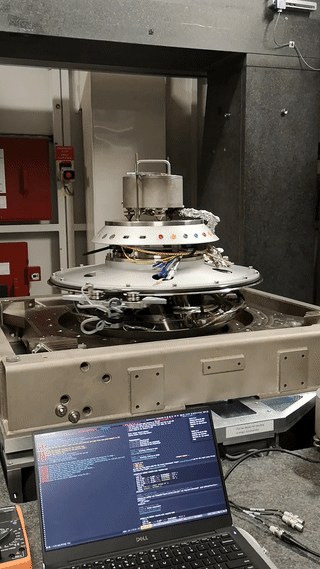
Experimental Setup
Setup: All the stages are OFF.
Two geophone are use:
- One on the marble (corresponding to the first column in the data)
- One at the sample location (corresponding to the second column in the data)
Two voltage amplifiers are used, their setup is:
- gain of 60dB
- AC/DC switch on AC
- Low pass filter at 1kHz
A first order low pass filter is also added at the input of the voltage amplifiers.
Goal:
- Identify the vibrations induced by the rotation of the Slip-Ring and Spindle
Measurements: Three measurements are done:
| Measurement File | Description |
|---|---|
mat/data_024.mat |
All the stages are OFF |
mat/data_025.mat |
The slip-ring is ON and rotates at 6rpm. The spindle is OFF |
mat/data_026.mat |
The slip-ring and spindle are both ON. They are both turning at 6rpm |
Each of the measurement mat file contains one data array with 3 columns:
| Column number | Description |
|---|---|
| 1 | Geophone - Marble |
| 2 | Geophone - Sample |
| 3 | Time |
A movie showing the experiment is shown on figure fig:exp_sl_sp_gif.
Data Analysis
<<sec:spindle_slip_ring_vibrations>>
ZIP file containing the data and matlab files ignore
All the files (data and Matlab scripts) are accessible here.
Load data
  of = load('mat/data_024.mat', 'data'); of = of.data; % OFF
  sr = load('mat/data_025.mat', 'data'); sr = sr.data; % Slip Ring
  sp = load('mat/data_026.mat', 'data'); sp = sp.data; % Spindle
There is a sign error for the Geophone located on top of the Hexapod. The problem probably comes from the wiring in the Slip-Ring.
  of(:, 2) = -of(:, 2);
  sr(:, 2) = -sr(:, 2);
  sp(:, 2) = -sp(:, 2);
Voltage to Velocity
We convert the measured voltage to velocity using the function voltageToVelocityL22 (accessible here).
  gain = 60; % [dB]

  of(:, 1) = voltageToVelocityL22(of(:, 1), of(:, 3), gain);
  sr(:, 1) = voltageToVelocityL22(sr(:, 1), sr(:, 3), gain);
  sp(:, 1) = voltageToVelocityL22(sp(:, 1), sp(:, 3), gain);

  of(:, 2) = voltageToVelocityL22(of(:, 2), of(:, 3), gain);
  sr(:, 2) = voltageToVelocityL22(sr(:, 2), sr(:, 3), gain);
  sp(:, 2) = voltageToVelocityL22(sp(:, 2), sp(:, 3), gain);
Time domain plots
  figure;
  hold on;
  plot(sp(:, 3), sp(:, 1), 'DisplayName', 'Spindle - 6rpm');
  plot(sr(:, 3), sr(:, 1), 'DisplayName', 'Slip-Ring - 6rpm');
  plot(of(:, 3), of(:, 1), 'DisplayName', 'OFF');
  hold off;
  xlabel('Time [s]'); ylabel('Velocity [m/s]');
  xlim([0, 100]);
legend('Location', 'northeast'); <<plt-matlab>>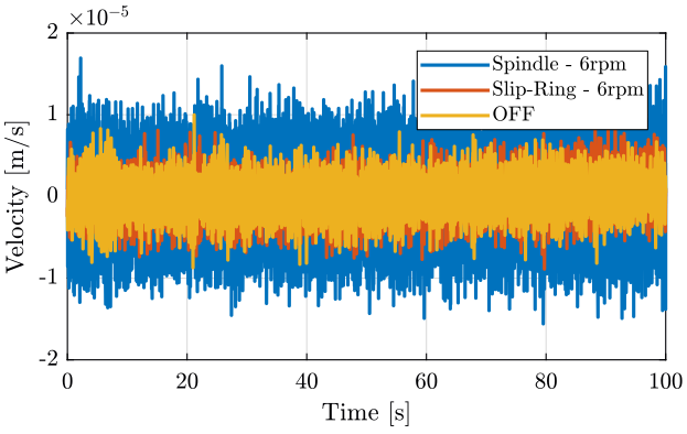
  figure;
  hold on;
  plot(sp(:, 3), sp(:, 2), 'DisplayName', 'Spindle and Slip-Ring');
  plot(sr(:, 3), sr(:, 2), 'DisplayName', 'Only Slip-Ring');
  plot(of(:, 3), of(:, 2), 'DisplayName', 'OFF');
  hold off;
  xlabel('Time [s]'); ylabel('Velocity [m/s]');
  xlim([0, 100]);
legend('Location', 'northeast'); <<plt-matlab>>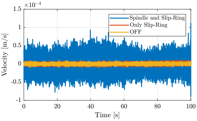
<<plt-matlab>>
Frequency Domain
We first compute some parameters that will be used for the PSD computation.
  dt = of(2, 3)-of(1, 3); % [s]

  Fs = 1/dt; % [Hz]

  win = hanning(ceil(10*Fs)); % Window used
Then we compute the Power Spectral Density using pwelch function.
First for the geophone located on the marble
  [pxof_m, f] = pwelch(of(:, 1), win, [], [], Fs);
  [pxsr_m, ~] = pwelch(sr(:, 1), win, [], [], Fs);
  [pxsp_m, ~] = pwelch(sp(:, 1), win, [], [], Fs);
And for the geophone located at the sample position.
  [pxof_s, ~] = pwelch(of(:, 2), win, [], [], Fs);
  [pxsr_s, ~] = pwelch(sr(:, 2), win, [], [], Fs);
  [pxsp_s, ~] = pwelch(sp(:, 2), win, [], [], Fs);
And we plot the ASD of the measured velocities:
- figure fig:sr_sp_psd_marble_compare for the geophone located on the marble
- figure fig:sr_sp_psd_sample_compare for the geophone at the sample position
  figure;
  hold on;
  plot(f, sqrt(pxsp_m), 'DisplayName', 'Spindle - 6rpm');
  plot(f, sqrt(pxsr_m), 'DisplayName', 'Slip-Ring - 6rpm');
  plot(f, sqrt(pxof_m), 'DisplayName', 'OFF');
  hold off;
  set(gca, 'xscale', 'log');
  set(gca, 'yscale', 'log');
  xlabel('Frequency [Hz]'); ylabel('ASD of the measured velocity $\left[\frac{m/s}{\sqrt{Hz}}\right]$')
  legend('Location', 'southwest');
xlim([2, 500]); <<plt-matlab>>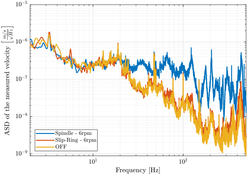
  figure;
  hold on;
  plot(f, sqrt(pxsp_s), 'DisplayName', 'Spindle - 6rpm');
  plot(f, sqrt(pxsr_s), 'DisplayName', 'Slip-Ring - 6rpm');
  plot(f, sqrt(pxof_s), 'DisplayName', 'OFF');
  hold off;
  set(gca, 'xscale', 'log');
  set(gca, 'yscale', 'log');
  xlabel('Frequency [Hz]'); ylabel('ASD of the measured velocity $\left[\frac{m/s}{\sqrt{Hz}}\right]$')
  legend('Location', 'southwest');
xlim([2, 500]); <<plt-matlab>>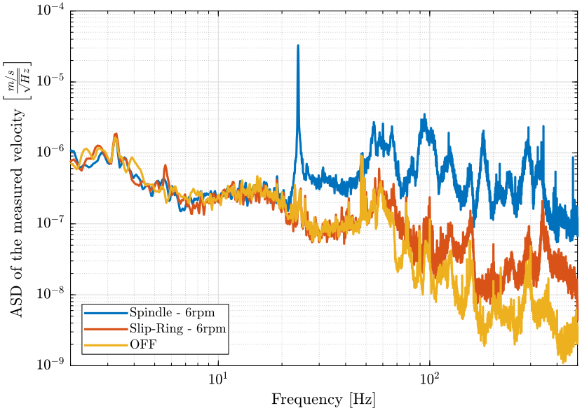
We load the ground motion to compare with the measurements (Fig. fig:ty_comp_gm). We see that the motion is dominated by the ground motion below 20Hz.
gm = load('../ground-motion/mat/psd_gm.mat', 'f', 'psd_gv'); figure;
hold on;
plot(f, sqrt(pxsp_m), 'DisplayName', 'Spindle - 6rpm');
plot(f, sqrt(pxsr_m), 'DisplayName', 'Slip-Ring - 6rpm');
plot(f, sqrt(pxof_m), 'DisplayName', 'OFF');
plot(gm.f, sqrt(gm.psd_gv), 'k-', 'DisplayName', 'Ground Motion');
hold off;
set(gca, 'xscale', 'log');
set(gca, 'yscale', 'log');
xlabel('Frequency [Hz]'); ylabel('ASD of the measured velocity $\left[\frac{m/s}{\sqrt{Hz}}\right]$')
legend('Location', 'southwest');
xlim([2, 500]); <<plt-matlab>>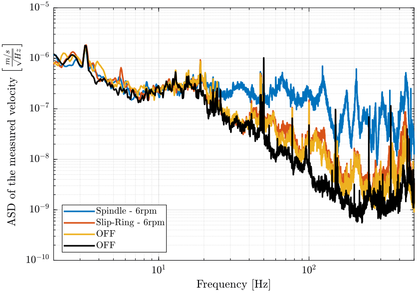
Relative Motion
The relative velocity between the sample and the marble is shown in Fig. fig:rz_relative_velocity. The velocity is integrated to have the relative displacement in Fig. fig:rz_relative_motion.
<<plt-matlab>>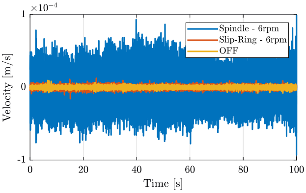
Time domain: Integration to have the displacement
<<plt-matlab>>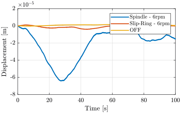
We compute the PSD of the relative velocity between the sample and the marble.
  [pxof_r, f] = pwelch(of(:, 2)-of(:, 1), win, [], [], Fs);
  [pxsr_r, ~] = pwelch(sr(:, 2)-sr(:, 1), win, [], [], Fs);
  [pxsp_r, ~] = pwelch(sp(:, 2)-sp(:, 1), win, [], [], Fs);
The Power Spectral Density of the Granite Velocity, Sample velocity and relative velocity are compare in Fig. fig:rz_psd_sample_granite_relative_comp.
<<plt-matlab>>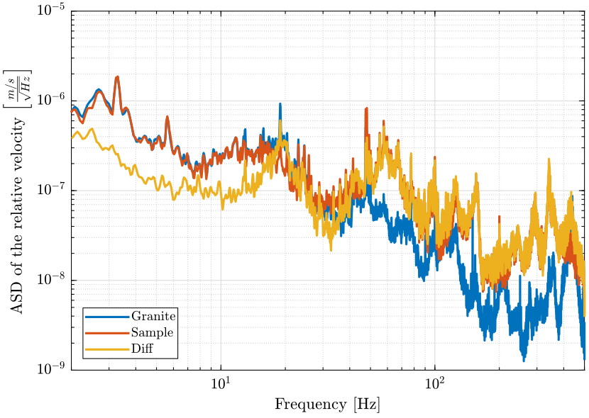
Then, we display the PSD of the relative velocity for all three cases in Fig. fig:sr_sp_psd_relative_compare.
  figure;
  hold on;
  plot(f, sqrt(pxsp_r), 'DisplayName', 'Spindle - 6rpm');
  plot(f, sqrt(pxsr_r), 'DisplayName', 'Slip-Ring - 6rpm');
  plot(f, sqrt(pxof_r), 'DisplayName', 'OFF');
  hold off;
  set(gca, 'xscale', 'log');
  set(gca, 'yscale', 'log');
  xlabel('Frequency [Hz]'); ylabel('ASD of the relative velocity $\left[\frac{m/s}{\sqrt{Hz}}\right]$')
  legend('Location', 'southwest');
xlim([2, 500]); <<plt-matlab>>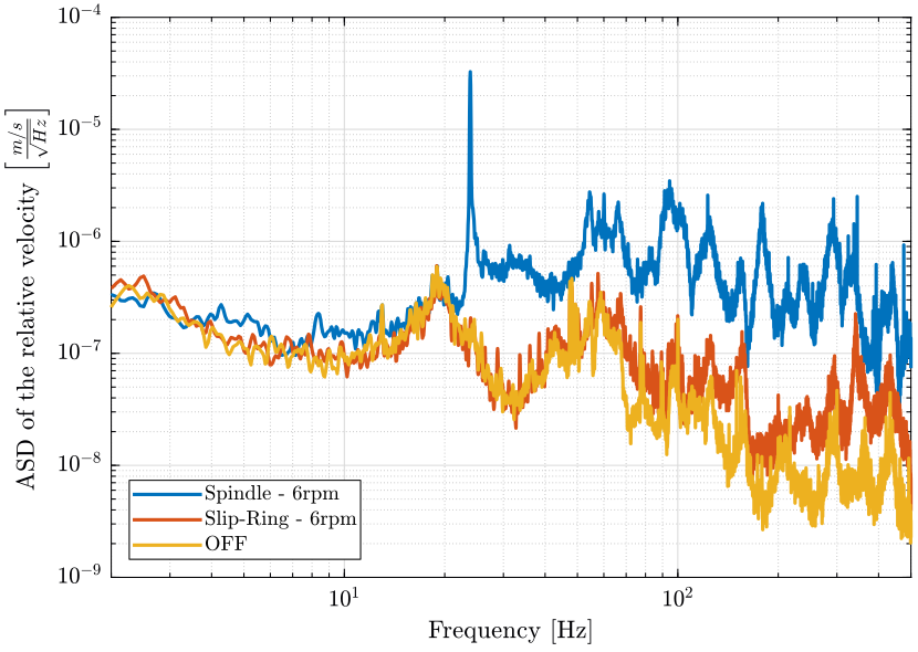
The Cumulative Power Spectrum of the relative velocity is shown in Fig. fig:dist_rz_cps and in Fig. fig:dist_rz_cps_reverse (integrated in reverse direction).
<<plt-matlab>>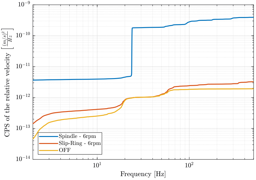
<<plt-matlab>>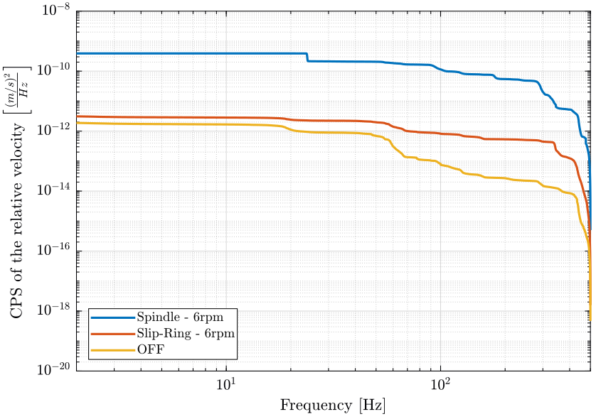
Finally, the Cumulative Amplitude Spectrum of the relative position between the hexapod and the marble is shown in Fig. fig:dist_rz_cas.
  figure;
  hold on;
  plot(f, sqrt(flip(-cumtrapz(flip(f), flip(pxsp_r./(2*pi*f).^2)))), 'DisplayName', 'Spindle - 6rpm');
  plot(f, sqrt(flip(-cumtrapz(flip(f), flip(pxsr_r./(2*pi*f).^2)))), 'DisplayName', 'Slip-Ring - 6rpm');
  plot(f, sqrt(flip(-cumtrapz(flip(f), flip(pxof_r./(2*pi*f).^2)))), 'DisplayName', 'OFF');
  hold off;
  set(gca, 'xscale', 'log'); set(gca, 'yscale', 'log');
  xlabel('Frequency [Hz]'); ylabel('CAS of the relative displacement $\left[\frac{m}{\sqrt{Hz}}\right]$')
  legend('Location', 'southwest');
xlim([2, 500]); <<plt-matlab>>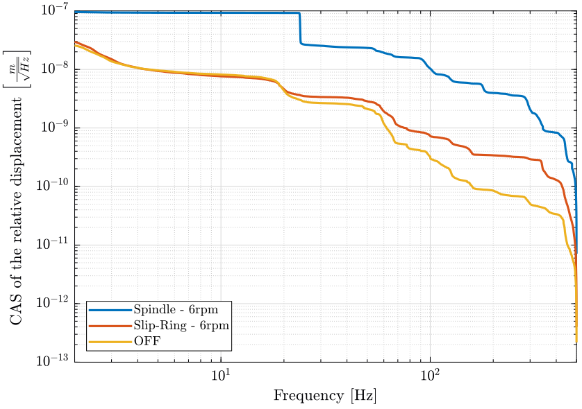
Save
The Power Spectral Density of the relative velocity and of the hexapod velocity is saved for further analysis.
save('mat/pxsp_r.mat', 'f', 'pxsp_r', 'pxsp_s');Conclusion
The relative motion below 20Hz is dominated by another effect than the rotation of the Spindle (probably ground motion).
The Slip-Ring rotation induce almost no relative motion of the hexapod with respect to the granite (only a little above 400Hz).
The Spindle rotation induces relative motion of the hexapod with respect to the granite above 20Hz.
There is a huge peak at 24Hz on the sample vibration but not on the granite vibration
- The peak is really sharp, could this be due to magnetic effect?
- Should redo the measurement with piezo accelerometers.