90 KiB
Modal Analysis - Modal Parameter Extraction
- ZIP file containing the data and matlab files
- Part to explain how to choose the modes frequencies
- Obtained Modal Parameters
- Obtained Mode Shapes animations
- Compute the Modal Model
- Problem with AirLoc System
- Setup
- Mode extraction and importation
- Positions of the sensors
- Solids
- From local coordinates to global coordinates for the mode shapes
- Modal Matrices
- Modal Complexity
- Some notes about constraining the number of degrees of freedom
- Normalization of mode shapes?
- Compare Mode Shapes
- Importation of measured FRF curves
- Importation of measured FRF curves to global FRF matrix
- Analysis of some FRFs
- Composite Response Function
- Singular Value Decomposition - Modal Indication Function
- From local coordinates to global coordinates with the FRFs
- Analysis of some FRF in the global coordinates
- Compare global coordinates to local coordinates
- Verify that we find the original FRF from the FRF in the global coordinates
- Synthesis of FRF curves
The goal here is to extract the modal parameters describing the modes of station being studied.
ZIP file containing the data and matlab files ignore
All the files (data and Matlab scripts) are accessible here.
TODO Part to explain how to choose the modes frequencies
- bro-band method used
- Stabilization Chart
- 21 modes
Obtained Modal Parameters
From the modal analysis software, we can export the obtained modal parameters:
- the resonance frequencies
- the modes shapes
- the modal damping
- the residues
These can be express as the eigen matrices: \[ \Omega = \begin{bmatrix} \omega_1^2 & & 0 \\ & \ddots & \\ 0 & & \omega_n^2 \end{bmatrix}; \quad \Psi = \begin{bmatrix} & & \\ \{\psi_1\} & \dots & \{\psi_n\} \\ & & \end{bmatrix} \] where $\bar{\omega}_r^2$ is the $r^\text{th}$ eigenvalue squared and $\{\phi\}_r$ is a description of the corresponding mode shape.
The file containing the modal parameters is mat/modes.asc. Its first 20 lines as shown below.
Created by N-Modal
Estimator: bbfd
01-Jul-19 16:44:11


Mode 1
freq    = 11.41275Hz
damp    = 8.72664%
modal A =  -4.50556e+003-9.41744e+003i
modal B =  -7.00928e+005+2.62922e+005i
Mode matrix of local coordinate [DOF: Re IM]
     1X-:  -1.04114e-001   3.50664e-002
     1Y-:   2.34008e-001   5.04273e-004
     1Z+:  -1.93303e-002   5.08614e-003
     2X-:  -8.38439e-002   3.45978e-002
     2Y-:   2.42440e-001   0.00000e+000
     2Z+:  -7.40734e-003   5.17734e-003
     3Y-:   2.17655e-001   6.10802e-003
     3X+:   1.18685e-001  -3.54602e-002
     3Z+:  -2.37725e-002  -1.61649e-003
We split this big modes.asc file into sub text files using bash. The obtained files are described one table tab:modes_files.
  sed '/^\s*[0-9]*[XYZ][+-]:/!d' mat/modes.asc > mat/mode_shapes.txt
  sed '/freq/!d'                 mat/modes.asc | sed 's/.* = \(.*\)Hz/\1/' > mat/mode_freqs.txt
  sed '/damp/!d'                 mat/modes.asc | sed 's/.* = \(.*\)\%/\1/' > mat/mode_damps.txt
  sed '/modal A/!d'              mat/modes.asc | sed 's/.* =\s\+\([-0-9.e]\++[0-9]\+\)\([-+0-9.e]\+\)i/\1 \2/' > mat/mode_modal_a.txt
sed '/modal B/!d' mat/modes.asc | sed 's/.* =\s\+\([-0-9.e]\++[0-9]\+\)\([-+0-9.e]\+\)i/\1 \2/' > mat/mode_modal_b.txt| Filename | Content |
|---|---|
mat/mode_shapes.txt |
mode shapes |
mat/mode_freqs.txt |
resonance frequencies |
mat/mode_damps.txt |
modal damping |
mat/mode_modal_a.txt |
modal residues at low frequency (to be checked) |
mat/mode_modal_b.txt |
modal residues at high frequency (to be checked) |
modes.asc file
Then we import the obtained .txt files on Matlab using readtable function.
  shapes  = readtable('mat/mode_shapes.txt',              'ReadVariableNames', false);  % [Sign / Real / Imag]
  freqs   = table2array(readtable('mat/mode_freqs.txt',   'ReadVariableNames', false)); % in [Hz]
  damps   = table2array(readtable('mat/mode_damps.txt',   'ReadVariableNames', false)); % in [%]
  modal_a = table2array(readtable('mat/mode_modal_a.txt', 'ReadVariableNames', false)); % [Real / Imag]
  modal_b = table2array(readtable('mat/mode_modal_b.txt', 'ReadVariableNames', false)); % [Real / Imag]

  modal_a = complex(modal_a(:, 1), modal_a(:, 2));
  modal_b = complex(modal_b(:, 1), modal_b(:, 2));
We guess the number of modes identified from the length of the imported data.
  acc_n = 23; % Number of accelerometers
  dir_n = 3; % Number of directions
  dirs = 'XYZ';

  mod_n = size(shapes,1)/acc_n/dir_n; % Number of modes
As the mode shapes are split into 3 parts (direction plus sign, real part and imaginary part), we aggregate them into one array of complex numbers.
  T_sign = table2array(shapes(:, 1));
  T_real = table2array(shapes(:, 2));
  T_imag = table2array(shapes(:, 3));

  modes = zeros(mod_n, acc_n, dir_n);

  for mod_i = 1:mod_n
    for acc_i = 1:acc_n
      % Get the correct section of the signs
      T = T_sign(acc_n*dir_n*(mod_i-1)+1:acc_n*dir_n*mod_i);
      for dir_i = 1:dir_n
        % Get the line corresponding to the sensor
        i = find(contains(T, sprintf('%i%s',acc_i, dirs(dir_i))), 1, 'first')+acc_n*dir_n*(mod_i-1);
        modes(mod_i, acc_i, dir_i) = str2num([T_sign{i}(end-1), '1'])*complex(T_real(i),T_imag(i));
      end
    end
  end
The obtained mode frequencies and damping are shown below.
data2orgtable([freqs, damps], {}, {'Frequency [Hz]', 'Damping [%]'}, ' %.1f ');| Frequency [Hz] | Damping [%] |
|---|---|
| 11.4 | 8.7 |
| 18.5 | 11.8 |
| 37.6 | 6.4 |
| 39.4 | 3.6 |
| 54.0 | 0.2 |
| 56.1 | 2.8 |
| 69.7 | 4.6 |
| 71.6 | 0.6 |
| 72.4 | 1.6 |
| 84.9 | 3.6 |
| 90.6 | 0.3 |
| 91.0 | 2.9 |
| 95.8 | 3.3 |
| 105.4 | 3.3 |
| 106.8 | 1.9 |
| 112.6 | 3.0 |
| 116.8 | 2.7 |
| 124.1 | 0.6 |
| 145.4 | 1.6 |
| 150.1 | 2.2 |
| 164.7 | 1.4 |
Obtained Mode Shapes animations
One all the FRFs are obtained, we can estimate the modal parameters (resonance frequencies, modal shapes and modal damping) within the modal software.
For that, multiple modal extraction techniques can be used (SIMO, MIMO, narrow band, wide band, …).
Then, it is possible to show the modal shapes with an animation.
Examples are shown on figures fig:mode1 and fig:mode6.
Animations of all the other modes are accessible using the following links: mode 1, mode 2, mode 3, mode 4, mode 5, mode 6, mode 7, mode 8, mode 9, mode 10, mode 11, mode 12, mode 13, mode 14, mode 15, mode 16, mode 17, mode 18, mode 19, mode 20, mode 21.
Compute the Modal Model
Position of the accelerometers
There are 23 accelerometers:
- 4 on the bottom granite
- 4 on the top granite
- 4 on top of the translation stage
- 4 on the tilt stage
- 3 on top of the spindle
- 4 on top of the hexapod
The coordinates defined in the software are displayed below.
     1  1.0000e-001  1.0000e-001  1.1500e+000      0          Top
     2  1.0000e-001 -1.0000e-001  1.1500e+000      0          Top
     3 -1.0000e-001 -1.0000e-001  1.1500e+000      0          Top
     4 -1.0000e-001  1.0000e-001  1.1500e+000      0          Top
     5  4.0000e-001  4.0000e-001  9.5000e-001      0        inner
     6  4.0000e-001 -4.0000e-001  9.5000e-001      0        inner
     7 -4.0000e-001 -4.0000e-001  9.5000e-001      0        inner
     8 -4.0000e-001  4.0000e-001  9.5000e-001      0        inner
     9  5.0000e-001  5.0000e-001  9.0000e-001      0        outer
    10  5.0000e-001 -5.0000e-001  9.0000e-001      0        outer
    11 -5.0000e-001 -5.0000e-001  9.0000e-001      0        outer
    12 -5.0000e-001  5.0000e-001  9.0000e-001      0        outer
    13  5.5000e-001  5.5000e-001  5.5000e-001      0          top
    14  5.5000e-001 -5.5000e-001  5.5000e-001      0          top
    15 -5.5000e-001 -5.5000e-001  5.5000e-001      0          top
    16 -5.5000e-001  5.5000e-001  5.5000e-001      0          top
    17  9.5000e-001  9.5000e-001  4.0000e-001      0          low
    18  9.5000e-001 -9.5000e-001  4.0000e-001      0          low
    19 -9.5000e-001 -9.5000e-001  4.0000e-001      0          low
    20 -9.5000e-001  9.5000e-001  4.0000e-001      0          low
    21  2.0000e-001  2.0000e-001  8.5000e-001      0          bot
    22  0.0000e+000 -2.0000e-001  8.5000e-001      0          bot
    23 -2.0000e-001  2.0000e-001  8.5000e-001      0          bot
| Node number | Solid Body | Location | X | Y | Z |
|---|---|---|---|---|---|
| 1 | Hexapod - Top | -X/-Y | -0.10 | -0.10 | 1.15 |
| 2 | -X/+Y | -0.10 | 0.10 | 1.15 | |
| 3 | +X/+Y | 0.10 | 0.10 | 1.15 | |
| 4 | +X/-Y | 0.10 | -0.10 | 1.15 | |
| 5 | Tilt - Top | -X/-Y | -0.40 | -0.40 | 0.95 |
| 6 | -X/+Y | -0.40 | 0.40 | 0.95 | |
| 7 | +X/+Y | 0.40 | 0.40 | 0.95 | |
| 8 | +X/-Y | 0.40 | -0.40 | 0.95 | |
| 9 | Translation - Top | -X/-Y | -0.50 | -0.50 | 0.90 |
| 10 | -X/+Y | -0.50 | 0.50 | 0.90 | |
| 11 | +X/+Y | 0.50 | 0.50 | 0.90 | |
| 12 | +X/-Y | 0.50 | -0.50 | 0.90 | |
| 13 | Top Granite | -X/-Y | -0.55 | -0.50 | 0.55 |
| 14 | -X/+Y | -0.55 | 0.50 | 0.55 | |
| 15 | +X/+Y | 0.55 | 0.50 | 0.55 | |
| 16 | +X/-Y | 0.55 | -0.50 | 0.55 | |
| 17 | Bottom Granite | -X/-Y | -0.95 | -0.90 | 0.40 |
| 18 | -X/+Y | -0.95 | 0.90 | 0.40 | |
| 19 | +X/+Y | 0.95 | 0.90 | 0.40 | |
| 20 | +X/-Y | 0.95 | -0.90 | 0.40 | |
| 21 | Spindle - Top | -X/-Y | -0.20 | -0.20 | 0.85 |
| 22 | +0/+Y | 0.00 | 0.20 | 0.85 | |
| 23 | +X/-Y | 0.20 | -0.20 | 0.85 |
Define positions of the accelerometers on matlab
We define the X-Y-Z position of each sensor. Each line corresponds to one accelerometer, X-Y-Z position in meter.
  positions = [...
    -0.10, -0.10, 1.15 ; ...
    -0.10,  0.10, 1.15 ; ...
     0.10,  0.10, 1.15 ; ...
     0.10, -0.10, 1.15 ; ...
    -0.40, -0.40, 0.95 ; ...
    -0.40,  0.40, 0.95 ; ...
     0.40,  0.40, 0.95 ; ...
     0.40, -0.40, 0.95 ; ...
    -0.50, -0.50, 0.90 ; ...
    -0.50,  0.50, 0.90 ; ...
     0.50,  0.50, 0.90 ; ...
     0.50, -0.50, 0.90 ; ...
    -0.55, -0.50, 0.55 ; ...
    -0.55,  0.50, 0.55 ; ...
     0.55,  0.50, 0.55 ; ...
     0.55, -0.50, 0.55 ; ...
    -0.95, -0.90, 0.40 ; ...
    -0.95,  0.90, 0.40 ; ...
     0.95,  0.90, 0.40 ; ...
     0.95, -0.90, 0.40 ; ...
    -0.20, -0.20, 0.85 ; ...
     0.00,  0.20, 0.85 ; ...
0.20, -0.20, 0.85 ]; figure;
hold on;
fill3(positions(1:4, 1), positions(1:4, 2), positions(1:4, 3), 'k', 'FaceAlpha', 0.5)
fill3(positions(5:8, 1), positions(5:8, 2), positions(5:8, 3), 'k', 'FaceAlpha', 0.5)
fill3(positions(9:12, 1), positions(9:12, 2), positions(9:12, 3), 'k', 'FaceAlpha', 0.5)
fill3(positions(13:16, 1), positions(13:16, 2), positions(13:16, 3), 'k', 'FaceAlpha', 0.5)
fill3(positions(17:20, 1), positions(17:20, 2), positions(17:20, 3), 'k', 'FaceAlpha', 0.5)
fill3(positions(21:23, 1), positions(21:23, 2), positions(21:23, 3), 'k', 'FaceAlpha', 0.5)
hold off;Import the modal vectors on matlab
Mode1
mode1 = [...
-9.34637e-002+j*4.52445e-002, +2.33790e-001+j*1.41439e-003, -1.73754e-002+j*6.02449e-003;
-7.42108e-002+j*3.91543e-002, +2.41566e-001-j*1.44869e-003, -5.99285e-003+j*2.10370e-003;
-9.40720e-002+j*3.93724e-002, +2.52307e-001+j*0.00000e+000, -1.53864e-002-j*9.25720e-004;
-1.02163e-001+j*2.79561e-002, +2.29048e-001+j*2.89782e-002, -2.85130e-002+j*1.77132e-004;
-8.77132e-002+j*3.34081e-002, +2.14182e-001+j*2.14655e-002, -1.54521e-002+j*1.26682e-002;
-7.90143e-002+j*2.42583e-002, +2.20669e-001+j*2.12738e-002, +4.60755e-002+j*4.96406e-003;
-7.79654e-002+j*2.58385e-002, +2.06861e-001+j*3.48019e-002, -1.78311e-002-j*1.29704e-002;
-8.49357e-002+j*3.55200e-002, +2.07470e-001+j*3.59745e-002, -7.66974e-002-j*3.19813e-003;
-7.38565e-002+j*1.95146e-002, +2.17403e-001+j*2.01550e-002, -1.77073e-002-j*3.46414e-003;
-7.77587e-002+j*2.36700e-002, +2.35654e-001-j*2.14540e-002, +7.94165e-002-j*2.45897e-002;
-8.17972e-002+j*2.20583e-002, +2.20906e-001-j*4.30164e-003, -5.60520e-003+j*3.10187e-003;
-8.64261e-002+j*3.66022e-002, +2.15000e-001-j*5.74661e-003, -1.22622e-001+j*4.11767e-002;
-4.25169e-002+j*1.56602e-002, +5.31036e-002-j*1.73951e-002, -4.07130e-002+j*1.26884e-002;
-3.85032e-002+j*1.29431e-002, +5.36716e-002-j*1.80868e-002, +1.00367e-001-j*3.48798e-002;
-4.25524e-002+j*1.46363e-002, +5.19668e-002-j*1.69744e-002, +5.89747e-003-j*2.32428e-003;
-4.31268e-002+j*1.38332e-002, +5.07545e-002-j*1.53045e-002, -1.04172e-001+j*3.17984e-002;
-2.69757e-002+j*9.07955e-003, +3.07837e-002-j*9.44663e-003, -7.63502e-003+j*1.68203e-003;
-3.00097e-002+j*9.23966e-003, +2.83585e-002-j*8.97747e-003, +1.52467e-001-j*4.78675e-002;
-2.70223e-002+j*6.16478e-003, +3.06149e-002-j*6.25382e-003, -4.84888e-003+j*1.93970e-003;
-2.90976e-002+j*7.13184e-003, +3.36738e-002-j*7.30875e-003, -1.66902e-001+j*3.93419e-002;
-7.91940e-002+j*4.39648e-002, +2.04567e-001+j*9.49987e-003, -1.56087e-002+j*7.08838e-003;
-1.01070e-001+j*3.13534e-002, +1.92270e-001+j*1.80423e-002, +2.93053e-003-j*1.97308e-003;
-8.86455e-002+j*4.29906e-002, +1.90862e-001+j*2.53414e-002, -3.38351e-002+j*1.81362e-003];Mode2
mode2 = [...
+7.56931e-002+j*3.61548e-002, +2.07574e-001+j*1.69205e-004, +1.29733e-002-j*6.78426e-004;
+8.58732e-002+j*2.54470e-002, +2.07117e-001-j*1.31755e-003, -2.13788e-003-j*1.24974e-002;
+8.17201e-002+j*2.36079e-002, +2.15927e-001+j*1.61300e-002, -5.48456e-004+j*2.55691e-002;
+7.09825e-002+j*3.66313e-002, +2.09969e-001+j*1.11484e-002, +9.19478e-003+j*3.47272e-002;
+6.23935e-002+j*1.02488e-002, +2.30687e-001-j*3.58416e-003, +3.27122e-002-j*5.85468e-002;
+7.61163e-002-j*2.43630e-002, +2.26743e-001-j*1.15334e-002, -6.20205e-003-j*1.21742e-001;
+8.01824e-002-j*1.94769e-002, +1.97485e-001+j*4.50105e-002, -2.21170e-002+j*9.77052e-002;
+6.19294e-002+j*8.15075e-003, +2.03864e-001+j*4.45835e-002, +2.55133e-002+j*1.36137e-001;
+4.38135e-002+j*7.30537e-002, +2.28426e-001-j*6.58868e-003, +1.16313e-002+j*5.09427e-004;
+5.45770e-002+j*4.34251e-002, +2.50823e-001+j*0.00000e+000, -4.63460e-002-j*4.76868e-002;
+5.50987e-002+j*4.26178e-002, +2.29394e-001+j*5.78236e-002, +1.90158e-002+j*1.09139e-002;
+4.98867e-002+j*7.30190e-002, +2.07871e-001+j*4.57750e-002, +6.69433e-002+j*9.00315e-002;
+2.48819e-002+j*3.03222e-002, -2.56046e-002-j*3.34132e-002, +2.13260e-002+j*2.58544e-002;
+2.45706e-002+j*2.60221e-002, -2.57723e-002-j*3.35612e-002, -5.71282e-002-j*6.61562e-002;
+2.68196e-002+j*2.83888e-002, -2.57263e-002-j*3.29627e-002, -2.11722e-003-j*3.37239e-003;
+2.51442e-002+j*3.32558e-002, -2.54372e-002-j*3.25062e-002, +5.65780e-002+j*7.64142e-002;
+1.62437e-002+j*1.94534e-002, -1.31293e-002-j*2.05924e-002, +1.05274e-003+j*3.59474e-003;
+1.83431e-002+j*2.03836e-002, -1.16818e-002-j*1.86334e-002, -8.66632e-002-j*1.08216e-001;
+1.62553e-002+j*1.79588e-002, -1.28857e-002-j*1.90512e-002, +6.25653e-003+j*4.97733e-003;
+1.63830e-002+j*2.03943e-002, -1.48941e-002-j*2.11717e-002, +8.68045e-002+j*1.16491e-001;
+6.79204e-002-j*5.55513e-002, +2.32871e-001+j*2.33389e-002, +1.34345e-002-j*2.31815e-002;
+4.02414e-002-j*8.38957e-002, +2.35273e-001+j*2.73256e-002, -8.51632e-003-j*7.49635e-003;
+6.18293e-002-j*5.99671e-002, +2.37693e-001+j*4.34204e-002, +1.63533e-002+j*6.09161e-002]Mode3
mode3 = [...
+1.34688e-001-j*6.65071e-002, +1.55316e-002+j*1.01277e-002, -5.88466e-002+j*1.14294e-002;
+1.53934e-001-j*9.76990e-003, +7.17487e-003+j*1.11925e-002, -4.57205e-002+j*7.26573e-003;
+1.61551e-001+j*1.65478e-002, -4.12527e-004-j*5.60909e-002, -9.00640e-003+j*3.50754e-003;
+1.37298e-001-j*5.24661e-002, +1.19427e-003-j*5.39240e-002, -1.25915e-002+j*5.38133e-003;
+2.43192e-001-j*3.17374e-002, -2.15730e-001-j*7.69941e-004, -1.56268e-001+j*1.44118e-002;
-7.27705e-002-j*3.54943e-003, -2.47706e-001+j*2.66480e-003, -1.21590e-001+j*1.06054e-002;
-7.25870e-002-j*4.62024e-003, +2.27073e-001-j*3.69315e-002, +1.22611e-001-j*6.67337e-003;
+2.32731e-001-j*2.85516e-002, +2.35389e-001-j*3.81905e-002, +5.35574e-002+j*4.30394e-004;
+2.64170e-001-j*2.67367e-002, -2.56227e-001+j*3.97957e-005, -1.95398e-001+j*2.23549e-002;
-1.66953e-002-j*7.95698e-003, -2.66547e-001-j*2.17687e-002, +1.56278e-002+j*2.23786e-003;
-3.42364e-002-j*9.30205e-003, +2.52340e-001-j*7.47237e-003, -9.51643e-004+j*3.64798e-003;
+2.97574e-001+j*0.00000e+000, +2.23170e-001-j*1.37831e-002, +1.06266e-001+j*2.30324e-003;
+2.67178e-002-j*4.15723e-004, +6.75423e-003-j*2.18428e-003, -1.69423e-002+j*3.12395e-003;
-1.12283e-002+j*2.86316e-004, +5.08225e-003-j*2.14053e-003, +2.18339e-002-j*3.25204e-003;
-1.17948e-002+j*6.82873e-004, +1.94914e-002-j*2.42151e-003, +2.68660e-003-j*2.92104e-004;
+1.19490e-002+j*1.72236e-005, +1.83552e-002-j*2.71289e-003, -2.70914e-002+j*4.84164e-003;
+1.00173e-002-j*5.80552e-005, -3.87262e-003-j*1.19607e-003, -8.53809e-003+j*1.48424e-003;
-1.22262e-002+j*5.13096e-004, -5.73905e-003-j*1.07659e-003, +3.51730e-002-j*6.13814e-003;
-1.43735e-002-j*4.78552e-004, +2.31135e-002-j*6.30554e-004, +1.80171e-003-j*1.98835e-004;
+9.17792e-003+j*5.36661e-004, +2.18969e-002-j*5.81759e-004, -3.72117e-002+j*5.35813e-003;
+3.38754e-002-j*3.38703e-002, -2.20843e-002+j*2.78581e-002, -8.79541e-002-j*3.67473e-003;
+3.93064e-002+j*4.69476e-002, -1.69132e-002-j*1.04606e-002, -1.85351e-002+j*1.33750e-003;
+3.60396e-002-j*2.46238e-002, -1.92038e-002-j*6.65895e-002, +3.57722e-003+j*3.64827e-003];Mode4
mode4 = [...
-1.02501e-001-j*1.43802e-001, -1.07971e-001+j*5.61418e-004, +1.87145e-001-j*1.03605e-001;
-9.44764e-002-j*1.36856e-001, -1.04428e-001+j*5.27790e-003, +1.60710e-001-j*7.74212e-002;
-9.11657e-002-j*1.36611e-001, -1.78165e-001-j*3.47193e-002, +2.37121e-001-j*4.96494e-002;
-9.17242e-002-j*1.36656e-001, -1.34249e-001-j*1.03884e-002, +1.92123e-001-j*1.25627e-001;
+1.05875e-002-j*1.03886e-001, -8.26338e-002+j*3.58498e-002, +2.55819e-001-j*6.94290e-003;
-4.58970e-002-j*1.33904e-002, -9.41660e-002+j*4.99682e-002, +1.28276e-001+j*4.59685e-002;
-6.01521e-002-j*1.30165e-002, +2.56439e-003-j*6.78141e-002, +5.03428e-002-j*1.59420e-001;
-1.00895e-002-j*8.80550e-002, +1.26327e-002-j*8.14444e-002, +1.59506e-001-j*2.05360e-001;
-3.04658e-003-j*1.57921e-001, -8.23501e-002+j*4.82748e-002, +1.69315e-001+j*1.22804e-002;
-8.25875e-002-j*7.31038e-002, -1.08668e-001+j*3.56364e-002, +8.28567e-002-j*4.49596e-003;
-1.06792e-001-j*6.95394e-002, +3.77195e-002-j*7.65410e-002, +8.00590e-003-j*2.32461e-002;
-4.84292e-002-j*1.45790e-001, +1.03862e-002-j*7.31212e-002, +1.78122e-001-j*1.00939e-001;
-3.49891e-002-j*6.20969e-003, -1.18504e-002-j*1.94225e-002, +4.13007e-002+j*7.67087e-003;
-3.55795e-002+j*1.16708e-003, -1.68128e-002-j*1.82344e-002, +3.92416e-002-j*3.64434e-002;
-3.45304e-002+j*3.78185e-003, -7.62559e-003-j*2.24241e-002, +6.28286e-003-j*1.32711e-002;
-9.95646e-003-j*6.04395e-003, -8.73465e-003-j*2.20807e-002, +3.56946e-002+j*1.69231e-002;
-9.32661e-003-j*5.51944e-003, -1.91087e-002-j*9.09191e-003, +4.04981e-002+j*8.38685e-004;
-2.84456e-002+j*4.02762e-003, -2.20044e-002-j*8.86197e-003, +4.43051e-002-j*5.21033e-002;
-3.27019e-002+j*3.59765e-003, +2.93163e-003-j*2.05064e-002, -1.77289e-002-j*1.29477e-002;
-1.08474e-002-j*5.78419e-003, +3.86759e-003-j*1.91642e-002, +2.10135e-002+j*3.18051e-002;
-1.34808e-002-j*9.69121e-003, +1.25218e-002-j*2.71411e-002, +2.76673e-001+j*0.00000e+000;
+1.96744e-003+j*4.90797e-003, -9.82609e-004-j*3.31065e-002, +1.79246e-001-j*3.33238e-002;
-1.08728e-002-j*8.80278e-003, -1.15217e-002-j*4.01143e-002, +2.30814e-001-j*8.33151e-002];All modes
mode_shapes = zeros(23, 3, 10);
mode_shapes(:, :, 1) = [...
-9.34637e-002+j*4.52445e-002, +2.33790e-001+j*1.41439e-003, -1.73754e-002+j*6.02449e-003;
-7.42108e-002+j*3.91543e-002, +2.41566e-001-j*1.44869e-003, -5.99285e-003+j*2.10370e-003;
-9.40720e-002+j*3.93724e-002, +2.52307e-001+j*0.00000e+000, -1.53864e-002-j*9.25720e-004;
-1.02163e-001+j*2.79561e-002, +2.29048e-001+j*2.89782e-002, -2.85130e-002+j*1.77132e-004;
-8.77132e-002+j*3.34081e-002, +2.14182e-001+j*2.14655e-002, -1.54521e-002+j*1.26682e-002;
-7.90143e-002+j*2.42583e-002, +2.20669e-001+j*2.12738e-002, +4.60755e-002+j*4.96406e-003;
-7.79654e-002+j*2.58385e-002, +2.06861e-001+j*3.48019e-002, -1.78311e-002-j*1.29704e-002;
-8.49357e-002+j*3.55200e-002, +2.07470e-001+j*3.59745e-002, -7.66974e-002-j*3.19813e-003;
-7.38565e-002+j*1.95146e-002, +2.17403e-001+j*2.01550e-002, -1.77073e-002-j*3.46414e-003;
-7.77587e-002+j*2.36700e-002, +2.35654e-001-j*2.14540e-002, +7.94165e-002-j*2.45897e-002;
-8.17972e-002+j*2.20583e-002, +2.20906e-001-j*4.30164e-003, -5.60520e-003+j*3.10187e-003;
-8.64261e-002+j*3.66022e-002, +2.15000e-001-j*5.74661e-003, -1.22622e-001+j*4.11767e-002;
-4.25169e-002+j*1.56602e-002, +5.31036e-002-j*1.73951e-002, -4.07130e-002+j*1.26884e-002;
-3.85032e-002+j*1.29431e-002, +5.36716e-002-j*1.80868e-002, +1.00367e-001-j*3.48798e-002;
-4.25524e-002+j*1.46363e-002, +5.19668e-002-j*1.69744e-002, +5.89747e-003-j*2.32428e-003;
-4.31268e-002+j*1.38332e-002, +5.07545e-002-j*1.53045e-002, -1.04172e-001+j*3.17984e-002;
-2.69757e-002+j*9.07955e-003, +3.07837e-002-j*9.44663e-003, -7.63502e-003+j*1.68203e-003;
-3.00097e-002+j*9.23966e-003, +2.83585e-002-j*8.97747e-003, +1.52467e-001-j*4.78675e-002;
-2.70223e-002+j*6.16478e-003, +3.06149e-002-j*6.25382e-003, -4.84888e-003+j*1.93970e-003;
-2.90976e-002+j*7.13184e-003, +3.36738e-002-j*7.30875e-003, -1.66902e-001+j*3.93419e-002;
-7.91940e-002+j*4.39648e-002, +2.04567e-001+j*9.49987e-003, -1.56087e-002+j*7.08838e-003;
-1.01070e-001+j*3.13534e-002, +1.92270e-001+j*1.80423e-002, +2.93053e-003-j*1.97308e-003;
-8.86455e-002+j*4.29906e-002, -3.38351e-002+j*1.81362e-003, +1.90862e-001+j*2.53414e-002];
mode_shapes(:, :, 2) = [...
+7.56931e-002+j*3.61548e-002, +2.07574e-001+j*1.69205e-004, +1.29733e-002-j*6.78426e-004;
+8.58732e-002+j*2.54470e-002, +2.07117e-001-j*1.31755e-003, -2.13788e-003-j*1.24974e-002;
+8.17201e-002+j*2.36079e-002, +2.15927e-001+j*1.61300e-002, -5.48456e-004+j*2.55691e-002;
+7.09825e-002+j*3.66313e-002, +2.09969e-001+j*1.11484e-002, +9.19478e-003+j*3.47272e-002;
+6.23935e-002+j*1.02488e-002, +2.30687e-001-j*3.58416e-003, +3.27122e-002-j*5.85468e-002;
+7.61163e-002-j*2.43630e-002, +2.26743e-001-j*1.15334e-002, -6.20205e-003-j*1.21742e-001;
+8.01824e-002-j*1.94769e-002, +1.97485e-001+j*4.50105e-002, -2.21170e-002+j*9.77052e-002;
+6.19294e-002+j*8.15075e-003, +2.03864e-001+j*4.45835e-002, +2.55133e-002+j*1.36137e-001;
+4.38135e-002+j*7.30537e-002, +2.28426e-001-j*6.58868e-003, +1.16313e-002+j*5.09427e-004;
+5.45770e-002+j*4.34251e-002, +2.50823e-001+j*0.00000e+000, -4.63460e-002-j*4.76868e-002;
+5.50987e-002+j*4.26178e-002, +2.29394e-001+j*5.78236e-002, +1.90158e-002+j*1.09139e-002;
+4.98867e-002+j*7.30190e-002, +2.07871e-001+j*4.57750e-002, +6.69433e-002+j*9.00315e-002;
+2.48819e-002+j*3.03222e-002, -2.56046e-002-j*3.34132e-002, +2.13260e-002+j*2.58544e-002;
+2.45706e-002+j*2.60221e-002, -2.57723e-002-j*3.35612e-002, -5.71282e-002-j*6.61562e-002;
+2.68196e-002+j*2.83888e-002, -2.57263e-002-j*3.29627e-002, -2.11722e-003-j*3.37239e-003;
+2.51442e-002+j*3.32558e-002, -2.54372e-002-j*3.25062e-002, +5.65780e-002+j*7.64142e-002;
+1.62437e-002+j*1.94534e-002, -1.31293e-002-j*2.05924e-002, +1.05274e-003+j*3.59474e-003;
+1.83431e-002+j*2.03836e-002, -1.16818e-002-j*1.86334e-002, -8.66632e-002-j*1.08216e-001;
+1.62553e-002+j*1.79588e-002, -1.28857e-002-j*1.90512e-002, +6.25653e-003+j*4.97733e-003;
+1.63830e-002+j*2.03943e-002, -1.48941e-002-j*2.11717e-002, +8.68045e-002+j*1.16491e-001;
+6.79204e-002-j*5.55513e-002, +2.32871e-001+j*2.33389e-002, +1.34345e-002-j*2.31815e-002;
+4.02414e-002-j*8.38957e-002, +2.35273e-001+j*2.73256e-002, -8.51632e-003-j*7.49635e-003;
+6.18293e-002-j*5.99671e-002, +1.63533e-002+j*6.09161e-002, +2.37693e-001+j*4.34204e-002];
mode_shapes(:, :, 3) = [...
+1.34688e-001-j*6.65071e-002, +1.55316e-002+j*1.01277e-002, -5.88466e-002+j*1.14294e-002;
+1.53934e-001-j*9.76990e-003, +7.17487e-003+j*1.11925e-002, -4.57205e-002+j*7.26573e-003;
+1.61551e-001+j*1.65478e-002, -4.12527e-004-j*5.60909e-002, -9.00640e-003+j*3.50754e-003;
+1.37298e-001-j*5.24661e-002, +1.19427e-003-j*5.39240e-002, -1.25915e-002+j*5.38133e-003;
+2.43192e-001-j*3.17374e-002, -2.15730e-001-j*7.69941e-004, -1.56268e-001+j*1.44118e-002;
-7.27705e-002-j*3.54943e-003, -2.47706e-001+j*2.66480e-003, -1.21590e-001+j*1.06054e-002;
-7.25870e-002-j*4.62024e-003, +2.27073e-001-j*3.69315e-002, +1.22611e-001-j*6.67337e-003;
+2.32731e-001-j*2.85516e-002, +2.35389e-001-j*3.81905e-002, +5.35574e-002+j*4.30394e-004;
+2.64170e-001-j*2.67367e-002, -2.56227e-001+j*3.97957e-005, -1.95398e-001+j*2.23549e-002;
-1.66953e-002-j*7.95698e-003, -2.66547e-001-j*2.17687e-002, +1.56278e-002+j*2.23786e-003;
-3.42364e-002-j*9.30205e-003, +2.52340e-001-j*7.47237e-003, -9.51643e-004+j*3.64798e-003;
+2.97574e-001+j*0.00000e+000, +2.23170e-001-j*1.37831e-002, +1.06266e-001+j*2.30324e-003;
+2.67178e-002-j*4.15723e-004, +6.75423e-003-j*2.18428e-003, -1.69423e-002+j*3.12395e-003;
-1.12283e-002+j*2.86316e-004, +5.08225e-003-j*2.14053e-003, +2.18339e-002-j*3.25204e-003;
-1.17948e-002+j*6.82873e-004, +1.94914e-002-j*2.42151e-003, +2.68660e-003-j*2.92104e-004;
+1.19490e-002+j*1.72236e-005, +1.83552e-002-j*2.71289e-003, -2.70914e-002+j*4.84164e-003;
+1.00173e-002-j*5.80552e-005, -3.87262e-003-j*1.19607e-003, -8.53809e-003+j*1.48424e-003;
-1.22262e-002+j*5.13096e-004, -5.73905e-003-j*1.07659e-003, +3.51730e-002-j*6.13814e-003;
-1.43735e-002-j*4.78552e-004, +2.31135e-002-j*6.30554e-004, +1.80171e-003-j*1.98835e-004;
+9.17792e-003+j*5.36661e-004, +2.18969e-002-j*5.81759e-004, -3.72117e-002+j*5.35813e-003;
+3.38754e-002-j*3.38703e-002, -2.20843e-002+j*2.78581e-002, -8.79541e-002-j*3.67473e-003;
+3.93064e-002+j*4.69476e-002, -1.69132e-002-j*1.04606e-002, -1.85351e-002+j*1.33750e-003;
+3.60396e-002-j*2.46238e-002, +3.57722e-003+j*3.64827e-003, -1.92038e-002-j*6.65895e-002];
mode_shapes(:, :, 4) = [...
-1.02501e-001-j*1.43802e-001, -1.07971e-001+j*5.61418e-004, +1.87145e-001-j*1.03605e-001;
-9.44764e-002-j*1.36856e-001, -1.04428e-001+j*5.27790e-003, +1.60710e-001-j*7.74212e-002;
-9.11657e-002-j*1.36611e-001, -1.78165e-001-j*3.47193e-002, +2.37121e-001-j*4.96494e-002;
-9.17242e-002-j*1.36656e-001, -1.34249e-001-j*1.03884e-002, +1.92123e-001-j*1.25627e-001;
+1.05875e-002-j*1.03886e-001, -8.26338e-002+j*3.58498e-002, +2.55819e-001-j*6.94290e-003;
-4.58970e-002-j*1.33904e-002, -9.41660e-002+j*4.99682e-002, +1.28276e-001+j*4.59685e-002;
-6.01521e-002-j*1.30165e-002, +2.56439e-003-j*6.78141e-002, +5.03428e-002-j*1.59420e-001;
-1.00895e-002-j*8.80550e-002, +1.26327e-002-j*8.14444e-002, +1.59506e-001-j*2.05360e-001;
-3.04658e-003-j*1.57921e-001, -8.23501e-002+j*4.82748e-002, +1.69315e-001+j*1.22804e-002;
-8.25875e-002-j*7.31038e-002, -1.08668e-001+j*3.56364e-002, +8.28567e-002-j*4.49596e-003;
-1.06792e-001-j*6.95394e-002, +3.77195e-002-j*7.65410e-002, +8.00590e-003-j*2.32461e-002;
-4.84292e-002-j*1.45790e-001, +1.03862e-002-j*7.31212e-002, +1.78122e-001-j*1.00939e-001;
-3.49891e-002-j*6.20969e-003, -1.18504e-002-j*1.94225e-002, +4.13007e-002+j*7.67087e-003;
-3.55795e-002+j*1.16708e-003, -1.68128e-002-j*1.82344e-002, +3.92416e-002-j*3.64434e-002;
-3.45304e-002+j*3.78185e-003, -7.62559e-003-j*2.24241e-002, +6.28286e-003-j*1.32711e-002;
-9.95646e-003-j*6.04395e-003, -8.73465e-003-j*2.20807e-002, +3.56946e-002+j*1.69231e-002;
-9.32661e-003-j*5.51944e-003, -1.91087e-002-j*9.09191e-003, +4.04981e-002+j*8.38685e-004;
-2.84456e-002+j*4.02762e-003, -2.20044e-002-j*8.86197e-003, +4.43051e-002-j*5.21033e-002;
-3.27019e-002+j*3.59765e-003, +2.93163e-003-j*2.05064e-002, -1.77289e-002-j*1.29477e-002;
-1.08474e-002-j*5.78419e-003, +3.86759e-003-j*1.91642e-002, +2.10135e-002+j*3.18051e-002;
-1.34808e-002-j*9.69121e-003, +1.25218e-002-j*2.71411e-002, +2.76673e-001+j*0.00000e+000;
+1.96744e-003+j*4.90797e-003, -9.82609e-004-j*3.31065e-002, +1.79246e-001-j*3.33238e-002;
-1.08728e-002-j*8.80278e-003, +2.30814e-001-j*8.33151e-002, -1.15217e-002-j*4.01143e-002];
mode_shapes(:, :, 5) = [...
+3.55328e-001+j*0.00000e+000, +6.67612e-002+j*5.48020e-002, +3.03237e-002+j*5.29473e-004;
+3.16372e-001-j*3.84091e-002, +5.27472e-002+j*5.88474e-002, +2.86305e-002-j*1.74805e-002;
+3.00803e-001-j*1.36309e-002, +7.04883e-002+j*1.24492e-001, +7.23329e-002+j*2.33738e-002;
+3.32527e-001-j*2.26876e-004, +9.82263e-002+j*1.20397e-001, +9.86580e-002+j*3.55048e-002;
+4.96498e-002+j*2.31008e-002, +9.79716e-002+j*1.42500e-002, -1.15121e-001-j*3.59085e-002;
+1.41924e-001+j*2.16209e-002, +8.76030e-002+j*6.39650e-003, -8.75727e-002-j*3.71261e-002;
+1.41522e-001+j*1.96964e-002, -1.01959e-001+j*4.10992e-004, +2.14744e-001+j*4.91249e-002;
+4.33170e-002+j*1.84481e-002, -8.24640e-002+j*3.42475e-003, +2.32281e-001+j*5.40699e-002;
+1.47782e-001+j*4.93091e-002, +8.75397e-002+j*7.75318e-004, -6.80833e-002-j*9.72902e-003;
+2.00055e-001+j*3.81689e-002, +8.06886e-002+j*1.19008e-002, -1.40810e-002-j*1.12625e-002;
+1.96526e-001+j*3.87737e-002, -8.42766e-002+j*9.20233e-003, +1.02951e-001+j*3.37680e-002;
+1.25035e-001+j*4.67796e-002, -8.81307e-002+j*5.81039e-004, +7.94320e-002+j*2.19736e-002;
+2.03946e-002+j*2.50162e-002, +7.93788e-002-j*1.40794e-002, -4.15470e-002+j*4.95855e-004;
+6.56876e-002-j*2.14826e-002, +8.21523e-002-j*1.94792e-002, +3.44089e-002+j*2.32727e-003;
+5.98960e-002-j*2.17160e-002, +4.74914e-002+j*2.31386e-002, +3.58704e-002+j*1.13591e-003;
+1.91580e-002+j*2.15329e-002, +5.14631e-002+j*1.70019e-002, -3.90820e-002-j*9.20853e-003;
+8.98876e-003+j*2.56390e-002, +7.93497e-002-j*2.34846e-002, -5.61039e-002-j*3.03271e-003;
+5.72051e-002-j*2.29477e-002, +8.76985e-002-j*2.73606e-002, +5.13896e-002+j*8.58341e-003;
+6.71099e-002-j*2.67997e-002, +1.80119e-002+j*4.02601e-002, +6.40092e-002+j*7.11273e-003;
+1.48349e-002+j*2.57533e-002, +1.35189e-002+j*3.69351e-002, -3.31024e-002-j*1.65471e-002;
+2.52156e-002-j*4.65138e-003, +7.94380e-004+j*1.56790e-002, +1.01067e-002-j*3.35468e-003;
+3.30841e-002+j*6.73531e-003, +1.69827e-004+j*9.48996e-003, +8.16746e-002+j*1.39885e-002;
+2.91404e-002-j*2.43138e-003, +1.38761e-001+j*3.67410e-002, -4.17833e-003+j*8.35629e-004];
mode_shapes(:, :, 6) = [...
+3.76055e-001-j*2.00477e-002, -2.18528e-002-j*2.46738e-001, -2.01369e-002-j*2.48481e-002;
+3.73870e-001-j*6.46353e-002, -3.66940e-002-j*2.49113e-001, -9.20410e-002-j*2.72520e-002;
+3.71070e-001-j*4.42411e-003, +5.79596e-002-j*2.58311e-001, +2.62275e-003+j*9.26708e-003;
+3.82440e-001+j*0.00000e+000, +3.30266e-002-j*2.08256e-001, +7.22558e-002+j*1.47204e-002;
-3.73785e-003+j*3.81592e-002, +4.74482e-002+j*5.41354e-002, -5.78227e-002-j*8.70215e-002;
+6.08721e-002+j*7.20835e-002, +5.73258e-002+j*5.38176e-002, -3.34121e-002-j*8.54509e-002;
+5.96968e-002+j*8.31733e-002, -7.64618e-002-j*4.19504e-002, +3.48953e-002+j*4.79635e-002;
-1.41532e-003+j*3.79318e-002, -6.79853e-002-j*3.88324e-002, +6.64542e-002+j*9.20955e-002;
+2.96044e-002+j*7.83613e-002, +4.91378e-002+j*4.74080e-002, -2.15758e-002-j*5.51292e-002;
+3.52566e-002+j*1.00976e-001, +4.16302e-002+j*5.95793e-002, -1.83944e-002-j*5.09313e-002;
+3.49287e-002+j*1.10404e-001, -5.46487e-002-j*3.95054e-002, +1.88545e-002+j*3.82156e-002;
+1.70173e-002+j*8.68762e-002, -5.52511e-002-j*4.46179e-002, +7.63555e-003+j*6.17646e-002;
-8.22469e-004-j*1.81402e-002, -1.96193e-003-j*2.76646e-002, -1.97033e-003+j*1.06615e-002;
-1.16438e-003-j*2.68725e-002, -1.11909e-003-j*2.38894e-002, +1.50332e-003+j*1.31644e-002;
-1.77060e-003-j*2.77807e-002, -1.01121e-003-j*2.37147e-002, -2.45798e-003-j*1.41886e-002;
-1.85500e-003-j*2.20304e-002, -4.77462e-004-j*2.19932e-002, -6.85097e-003-j*7.04903e-003;
-6.77197e-004-j*1.56812e-002, -2.19412e-003-j*2.65284e-002, +3.96653e-004+j*2.95178e-002;
-1.14513e-003-j*1.99551e-002, -2.35828e-003-j*2.88909e-002, +3.70211e-003+j*2.02423e-002;
-1.16798e-003-j*2.31638e-002, -4.75969e-004-j*2.23413e-002, -2.07031e-003-j*3.41651e-002;
-1.99807e-004-j*2.09301e-002, -2.40560e-004-j*1.78264e-002, -9.91090e-003-j*3.12664e-002;
+9.69966e-003+j*2.95222e-002, -1.19231e-002+j*5.23077e-003, -9.79113e-003-j*4.50715e-002;
+1.36018e-002+j*2.24850e-002, -9.79427e-003+j*9.84679e-003, +2.18456e-002-j*1.57858e-002;
+1.09214e-002+j*2.93115e-002, +2.43859e-002+j*3.35745e-002, -1.07735e-002+j*1.21178e-002];
mode_shapes(:, :, 7) = [...
+4.18739e-001-j*2.21696e-002, +6.52636e-002-j*1.29498e-001, -1.90337e-002+j*9.61505e-003;
+4.27024e-001-j*3.03566e-002, +4.22791e-002-j*1.32892e-001, -1.65941e-002+j*2.17638e-002;
+4.66694e-001+j*1.38778e-017, +7.51273e-002-j*1.57468e-001, -2.91618e-002+j*4.11516e-002;
+4.18867e-001+j*2.39590e-002, +7.51007e-002-j*1.13378e-001, -7.11238e-003+j*2.72692e-002;
-3.26299e-002+j*2.12910e-002, -4.80710e-002+j*8.82799e-002, +5.82558e-002-j*9.16159e-002;
-4.61031e-002+j*8.08300e-002, -2.80650e-002+j*7.37925e-002, +3.54903e-002-j*3.02341e-002;
-5.14543e-002+j*7.23863e-002, +1.91387e-002-j*7.65710e-002, -3.92182e-002+j*5.06089e-002;
-3.35647e-002+j*2.16695e-002, +1.88798e-002-j*6.19822e-002, -5.08508e-002+j*8.78653e-002;
-4.93941e-002+j*6.46940e-002, -2.90637e-002+j*7.66360e-002, +5.24626e-002-j*6.16359e-002;
-5.85364e-002+j*5.59044e-002, -2.63581e-002+j*5.43466e-002, +2.90174e-002-j*3.98049e-002;
-6.07978e-002+j*5.54585e-002, +3.16828e-002-j*8.54810e-002, -3.44914e-002-j*4.03684e-003;
-6.18120e-002+j*7.90821e-002, +2.38807e-002-j*5.62399e-002, -5.04609e-002+j*3.27008e-002;
+1.57670e-002-j*3.20728e-003, -5.98007e-003-j*3.10416e-003, -1.67104e-003-j*1.59089e-003;
+1.79638e-002-j*7.40235e-003, -8.20109e-003-j*2.36675e-004, -1.69812e-003+j*1.67596e-003;
+1.87809e-002-j*8.55724e-003, -2.81069e-003-j*3.03393e-003, -5.71319e-003-j*2.26161e-003;
+1.88829e-002-j*8.50228e-003, -5.28373e-003-j*2.52386e-003, -1.48737e-002-j*5.08140e-003;
+2.28380e-002-j*7.51769e-003, -7.57170e-003-j*2.75553e-003, -6.10380e-003+j*5.15562e-003;
+2.08600e-002-j*6.11732e-003, -4.73105e-003-j*3.30979e-003, -2.51369e-003+j*5.42921e-003;
+2.00008e-002-j*5.92617e-003, -3.50988e-003-j*4.55853e-003, -5.43701e-003-j*6.57229e-003;
+2.28149e-002-j*8.22905e-003, -4.83167e-003-j*3.10509e-003, -2.10958e-002-j*1.33421e-002;
-1.83145e-002+j*2.76844e-002, +5.61668e-003-j*1.41226e-002, +2.20876e-002-j*2.27446e-002;
-5.42112e-003+j*2.22444e-002, -4.20426e-005-j*8.78901e-003, +5.54714e-003+j*2.71564e-002;
-1.70108e-002+j*2.83751e-002, -1.44473e-002+j*4.50880e-002, -5.26736e-003-j*5.75716e-003];
mode_shapes(:, :, 8) = [...
-1.40928e-001+j*1.28570e-001, +2.95471e-001-j*1.35692e-001, -6.61656e-002+j*2.95705e-002;
-1.56673e-001+j*5.19030e-002, +3.08231e-001-j*1.41453e-001, -9.70918e-002+j*4.95018e-002;
-1.72505e-001+j*2.26273e-002, +3.97224e-001-j*2.77556e-017, -1.29223e-001+j*4.47412e-002;
-1.69978e-001+j*1.16284e-001, +3.37516e-001+j*7.69873e-003, -8.49480e-002+j*2.17071e-002;
+5.38303e-004-j*3.59916e-003, -6.72455e-002-j*2.06230e-002, +2.66448e-002+j*4.10505e-002;
-7.96526e-003-j*7.76851e-002, -2.63530e-002-j*3.75474e-002, -1.05984e-001+j*9.32474e-002;
+4.72518e-002-j*1.00199e-001, -5.50664e-002+j*1.50246e-001, -8.50976e-002+j*2.78531e-002;
+7.58419e-003-j*8.61594e-003, -9.02101e-002+j*1.58224e-001, +6.03081e-002-j*1.24162e-001;
+2.99027e-002-j*5.27128e-002, -8.80464e-002-j*2.99113e-004, +9.02851e-002-j*3.99771e-002;
+3.23132e-002-j*5.87278e-002, +3.81174e-002-j*3.69992e-002, +1.16643e-002+j*6.21068e-002;
+5.79795e-002-j*8.33565e-002, -1.22448e-003+j*8.81473e-002, +8.40150e-002-j*1.16264e-002;
+1.35399e-002-j*3.80303e-002, -9.58200e-002+j*1.46531e-001, +1.06769e-001-j*8.97034e-002;
+5.34299e-004+j*1.35179e-002, +8.71327e-004-j*6.41448e-003, +3.33208e-002-j*2.12545e-002;
-2.79263e-004+j*5.08578e-003, -1.45476e-003-j*7.65161e-003, +6.98235e-002-j*2.45395e-002;
-9.22822e-005+j*7.03205e-003, -5.62836e-003-j*2.79991e-003, +3.99717e-002-j*8.30891e-003;
+1.87833e-002+j*3.26772e-003, -4.86774e-003-j*4.32297e-003, +5.97375e-002-j*1.77542e-002;
+1.14169e-002+j*5.70930e-003, -8.23489e-003-j*4.53684e-003, +3.14016e-002-j*2.50637e-002;
+1.15995e-003+j*5.79180e-003, -6.69740e-003-j*4.66433e-003, +8.17695e-002-j*2.78384e-002;
+5.23838e-004+j*6.46432e-003, +3.36104e-003-j*4.42572e-003, +3.64589e-002+j*5.74796e-004;
+1.57042e-002+j*5.94177e-003, -1.49670e-003-j*4.22955e-003, +8.68520e-002-j*1.43981e-002;
+8.00706e-004-j*2.91734e-002, +1.20708e-002+j*4.24081e-002, -5.91796e-002+j*4.00346e-002;
-1.91799e-003-j*1.37294e-002, +9.85285e-003+j*3.17934e-002, -1.78010e-001+j*7.91267e-002;
+3.57271e-003-j*3.09959e-002, -5.77781e-002-j*1.27957e-002, +1.31025e-002+j*1.92303e-002];
mode_shapes(:, :, 9) = [...
+1.58897e-002+j*3.23763e-002, -1.23332e-001-j*3.20376e-002, +6.78860e-002-j*1.28743e-002;
+5.67179e-003+j*4.26539e-002, -1.20726e-001-j*4.15603e-002, +7.66846e-002-j*1.24290e-002;
+2.24198e-002+j*3.45953e-002, -1.03213e-001-j*4.97049e-002, +5.49175e-002-j*5.50883e-003;
+2.68792e-002+j*2.97222e-002, -1.17598e-001-j*3.13791e-002, +5.59736e-002-j*1.71122e-002;
+1.39733e-002-j*1.56260e-002, +1.43952e-001+j*2.28119e-002, -4.56377e-003+j*4.88790e-002;
-2.18507e-002-j*1.25664e-002, +6.15387e-002-j*6.31793e-003, +3.05342e-002+j*3.24595e-002;
-7.85412e-003-j*1.85600e-002, +1.25733e-001+j*1.77063e-002, +5.34635e-002+j*4.72260e-003;
-1.10454e-002-j*2.13217e-002, +1.26440e-001+j*1.96001e-002, -5.62624e-002-j*1.07192e-002;
+5.84467e-003-j*4.07134e-002, +5.16711e-003+j*4.70857e-002, -1.93010e-001+j*6.79213e-003;
+5.31962e-002-j*1.11322e-002, +3.23294e-001-j*2.12981e-002, +2.14310e-001+j*4.85898e-003;
-2.44580e-002-j*1.33220e-002, +4.08800e-001+j*2.09082e-002, +5.11454e-001+j*0.00000e+000;
-2.51332e-002-j*1.42719e-003, +8.97105e-002+j*4.85852e-002, -1.27426e-001-j*9.59723e-003;
-2.08176e-003+j*1.37185e-002, -3.99530e-002+j*2.11895e-002, -1.17813e-001+j*7.60972e-002;
-1.34824e-002+j*7.11258e-003, -4.19473e-002+j*1.83590e-002, -2.07198e-002-j*2.51991e-002;
-6.84747e-003+j*8.45921e-003, -3.33872e-002+j*1.71496e-002, +6.99867e-002-j*6.93158e-002;
-2.64313e-002+j*5.08903e-003, -3.03569e-002+j*1.29946e-002, -1.39115e-001+j*5.72459e-002;
-2.90186e-002+j*1.48257e-002, -5.55429e-002+j*2.74156e-002, -1.62035e-001+j*8.04187e-002;
-2.05855e-002+j*1.11922e-002, -6.58789e-002+j*3.20524e-002, -1.02263e-002-j*4.24087e-002;
-1.40204e-002+j*8.01102e-003, -5.72647e-002+j*2.37484e-002, +1.75053e-001-j*9.63667e-002;
-3.50818e-002+j*1.41152e-002, -5.19701e-002+j*2.31951e-002, -1.15951e-001+j*2.91582e-002;
-5.78005e-003-j*7.05841e-003, +8.29016e-002+j*1.36984e-002, +4.03470e-003+j*4.03325e-002;
-1.39928e-002-j*1.14088e-002, +8.05288e-002+j*1.51031e-002, +1.12255e-002+j*3.21224e-002;
-1.02276e-002-j*8.35724e-003, -4.89246e-003+j*1.67800e-002, +7.80514e-002+j*1.53467e-002];
mode_shapes(:, :, 10) = [...
+3.33349e-002-j*4.89606e-003, -8.67138e-002-j*1.69402e-002, +2.87366e-002-j*1.66842e-002;
+2.95730e-002-j*6.10477e-004, -9.24590e-002-j*1.92562e-002, +5.21162e-002-j*1.31811e-002;
+3.26966e-002+j*1.03975e-002, -8.55682e-002-j*4.71847e-002, +3.99404e-002+j*8.59358e-003;
+3.45452e-002-j*3.05951e-003, -7.73823e-002-j*2.32199e-002, +2.30960e-002-j*7.49928e-003;
-3.72461e-003-j*5.40336e-003, +1.80151e-001-j*1.42898e-002, -8.63921e-003+j*1.95638e-002;
-1.11285e-002-j*2.22175e-003, +6.92355e-002-j*1.24144e-002, +8.02097e-002-j*6.81531e-003;
-2.99885e-002-j*4.21951e-004, +8.19709e-002+j*1.22484e-002, +3.97531e-002+j*1.33874e-002;
-1.59231e-002-j*3.96929e-003, +9.31295e-002+j*9.75532e-003, -4.01947e-002-j*5.17841e-003;
-7.32828e-003-j*2.93496e-002, +4.39909e-002+j*1.25298e-002, -8.87525e-002+j*2.05359e-002;
+8.20167e-002+j*6.86693e-004, +4.25475e-001-j*2.36494e-002, +3.37034e-001-j*2.44199e-002;
-2.68694e-002+j*3.82921e-003, +4.79292e-001+j*1.35903e-002, +5.06762e-001+j*0.00000e+000;
+1.40565e-002-j*5.41957e-003, +1.17563e-001+j*2.50398e-002, -5.97219e-002+j*5.92813e-004;
+2.30939e-002+j*1.16755e-002, +4.11136e-003+j*1.65726e-002, +2.41863e-002+j*5.06658e-002;
-4.92960e-003+j*9.24082e-003, -5.44667e-003+j*1.41983e-002, -3.73537e-002-j*1.87263e-002;
+9.68682e-003+j*1.11791e-002, -5.13436e-003+j*1.29205e-002, -4.88765e-002-j*4.97821e-002;
-1.66711e-003+j*1.03280e-002, +9.57955e-004+j*1.28350e-002, +3.30268e-002+j*5.44211e-002;
+5.90540e-003+j*1.67113e-002, +1.34280e-002+j*2.62111e-002, +4.38613e-002+j*7.17028e-002;
+4.97752e-003+j*1.47634e-002, +1.56773e-002+j*3.16026e-002, -5.27493e-002-j*3.38315e-002;
+2.83485e-003+j*1.14816e-002, +9.80676e-003+j*2.51504e-002, -6.78645e-002-j*9.90875e-002;
+5.62294e-003+j*1.84035e-002, +1.03717e-002+j*2.37801e-002, +2.58497e-002+j*3.75352e-002;
-8.75236e-003-j*4.71723e-003, +6.99107e-002+j*1.51894e-002, +3.46273e-002+j*1.48547e-002;
-1.72822e-002-j*8.75192e-003, +6.96759e-002+j*1.59783e-002, +8.07917e-002+j*1.97809e-002;
-1.29601e-002-j*5.61834e-003, +1.76126e-002+j*4.62761e-003, +6.64667e-002+j*1.61199e-002];Define a point for each solid body
We define accelerometer indices used to define the motion of each solid body (2 3-axis accelerometer are enough).
stages = [17, 19; % Bottom Granite
13, 15; % Top Granite
9, 11; % Ty
5, 7; % Ry
21, 22; % Spindle
1, 3]; % HexapodWe define the origin point ${}^AO_B$ of the solid body $\{B\}$. Here we choose the middle point between the two accelerometers. This could be define differently (for instance by choosing the center of mass).
AOB = zeros(3, size(stages, 1));
for i = 1:size(stages, 1)
AOB(:, i) = mean(positions(stages(i, :), 1:3))';
endThen we compute the positions of the sensors with respect to the previously defined origin for the frame $\{B\}$: ${}^BP_1$ and ${}^BP_2$.
BP1 = zeros(3, size(stages, 1));
BP2 = zeros(3, size(stages, 1));
for i = 1:size(stages, 1)
BP1(:, i) = positions(stages(i, 1), 1:3)' - AOB(:, i);
BP2(:, i) = positions(stages(i, 2), 1:3)' - AOB(:, i);
endLet's define one absolute frame $\{A\}$ and one frame $\{B\}$ fixed w.r.t. the solid body. We note ${}^AO_B$ the position of origin of $\{B\}$ expressed in $\{A\}$.
We are measuring with the accelerometers the absolute motion of points $P_1$ and $P_2$: ${}^Av_{P_1}$ and ${}^Av_{P_2}$.
Let's note ${}^BP_1$ and ${}^BP_2$ the (known) coordinates of $P_1$ and $P_2$ expressed in the frame $\{B\}$.
Then we have:
\begin{align} {}^Av_{P_1} &= {}^Av_{O_B} + {}^A\Omega^\times {}^AR_B {}^BP_1 \\ {}^Av_{P_2} &= {}^Av_{O_B} + {}^A\Omega^\times {}^AR_B {}^BP_2 \end{align}And we obtain
\begin{align} {}^A\Omega^\times {}^AR_B &= \left( {}^Av_{P_2} - {}^Av_{P_1} \right) \left( {}^BP_2 - {}^BP_1 \right)^{-1}\\ {}^Av_{O_B} &= {}^Av_{P_1} - \left( {}^Av_{P_2} - {}^Av_{P_1} \right) \left( {}^BP_2 - {}^BP_1 \right)^{-1} {}^BP_1 \end{align} AVOB = zeros(3, size(stages, 1));
ARB = zeros(3, 3, size(stages, 1));
for i = 1:size(stages, 1)
AVOB(:, i) = mode1(stages(i, 1), :)' - (mode1(stages(i, 2), :)' - mode1(stages(i, 1), :)')*pinv(BP2(:, i) - BP1(:, i))*BP1(:, i);
ARB(:, :, i) = (mode1(stages(i, 2), :)' - mode1(stages(i, 1), :)')*pinv(BP2(:, i) - BP1(:, i));
endArgand Diagram
For mode 1
figure;
hold on;
for i=1:size(mode1, 1)
plot([0, real(mode1(i, 1))], [0, imag(mode1(i, 1))], '-k')
plot([0, real(mode1(i, 2))], [0, imag(mode1(i, 2))], '-k')
plot([0, real(mode1(i, 3))], [0, imag(mode1(i, 3))], '-k')
% plot([0, real(mode2(i, 1))], [0, imag(mode2(i, 1))], '-r')
% plot([0, real(mode2(i, 2))], [0, imag(mode2(i, 2))], '-r')
% plot([0, real(mode2(i, 3))], [0, imag(mode2(i, 3))], '-r')
% plot([0, real(mode3(i, 1))], [0, imag(mode3(i, 1))], '-b')
% plot([0, real(mode3(i, 2))], [0, imag(mode3(i, 2))], '-b')
% plot([0, real(mode3(i, 3))], [0, imag(mode3(i, 3))], '-b')
end
for i=1:size(AVOB, 2)
plot([0, real(AVOB(1, i))], [0, imag(AVOB(1, i))], '-r')
plot([0, real(AVOB(2, i))], [0, imag(AVOB(2, i))], '-r')
plot([0, real(AVOB(3, i))], [0, imag(AVOB(3, i))], '-r')
end
% ang=0:0.01:2*pi;
% radius1 = max(max(sqrt(real(mode1).^2+imag(mode1).^2)));
% plot(radius1*cos(ang), radius1*sin(ang), '-k');
% radius2 = max(max(sqrt(real(mode2).^2+imag(mode2).^2)));
% plot(radius2*cos(ang), radius2*sin(ang), '-r');
% radius3 = max(max(sqrt(real(mode3).^2+imag(mode3).^2)));
% plot(radius3*cos(ang), radius3*sin(ang), '-b');
hold off;
axis manual equalTEST: animate first mode
  figure;
  hold on;
  fill3(positions(1:4, 1),   positions(1:4, 2),   positions(1:4, 3),   'k', 'FaceAlpha', 0.5)
  fill3(positions(5:8, 1),   positions(5:8, 2),   positions(5:8, 3),   'k', 'FaceAlpha', 0.5)
  fill3(positions(9:12, 1),  positions(9:12, 2),  positions(9:12, 3),  'k', 'FaceAlpha', 0.5)
  fill3(positions(13:16, 1), positions(13:16, 2), positions(13:16, 3), 'k', 'FaceAlpha', 0.5)
  fill3(positions(17:20, 1), positions(17:20, 2), positions(17:20, 3), 'k', 'FaceAlpha', 0.5)
  fill3(positions(21:23, 1), positions(21:23, 2), positions(21:23, 3), 'k', 'FaceAlpha', 0.5)
hold off; rec = polyshape([-2 -2 2 2],[-3 3 3 -3]);
h = figure;
filename = 'figs/mode_shapes.gif';
n = 20;
for i = 1:n
axis manual equal
Dm = real(V(1:3, 5)*cos(2*pi*i/n));
rec_i = rotate(rec, 180/pi*Dm(3));
rec_i = translate(rec_i, 10*Dm(1), 10*Dm(2));
plot(rec_i);
xlim([-3, 3]); ylim([-4, 4]);
set(h, 'visible', 'off');
set(h, 'pos', [0, 0, 500, 500]);
drawnow;
% Capture the plot as an image
frame = getframe(h);
im = frame2im(frame);
[imind,cm] = rgb2ind(im,256);
% Write to the GIF File
if i == 1
imwrite(imind,cm,filename,'gif','DelayTime',0.1,'Loopcount',inf);
else
imwrite(imind,cm,filename,'gif','DelayTime',0.1,'WriteMode','append');
end
end
set(h, 'visible', 'on');
ans = filename;From 6 translations to translation + rotation
Let's define one absolute frame $\{A\}$ and one frame $\{B\}$ fixed w.r.t. the solid body. We note ${}^AO_B$ the position of origin of $\{B\}$ expressed in $\{A\}$.
We are measuring with the accelerometers the absolute motion of points $P_1$ and $P_2$: ${}^AP_1$ and ${}^AP_2$.
Let's note ${}^BP_1$ and ${}^BP_2$ the (known) coordinates of $P_1$ and $P_2$ expressed in the frame $\{B\}$.
Then we have:
\begin{align} {}^AP_1 &= {}^AO_B + {}^AR_B {}^BP_1 \\ {}^AP_2 &= {}^AO_B + {}^AR_B {}^BP_2 \end{align}And we obtain
\begin{align} {}^AR_B &= \left( {}^AP_2 - {}^AP_1 \right) \left( {}^BP_2 - {}^BP_1 \right)^{-1}\\ {}^AO_B &= {}^Av_{P_1} - \left( {}^AP_2 - {}^AP_1 \right) \left( {}^BP_2 - {}^BP_1 \right)^{-1} {}^BP_1 \end{align}Problem with AirLoc System
The mode shape of the first mode at 11Hz (figure fig:mode1) seems to indicate that this corresponds to a suspension mode.
This could be due to the 4 Airloc Levelers that are used for the granite (figure fig:airloc).
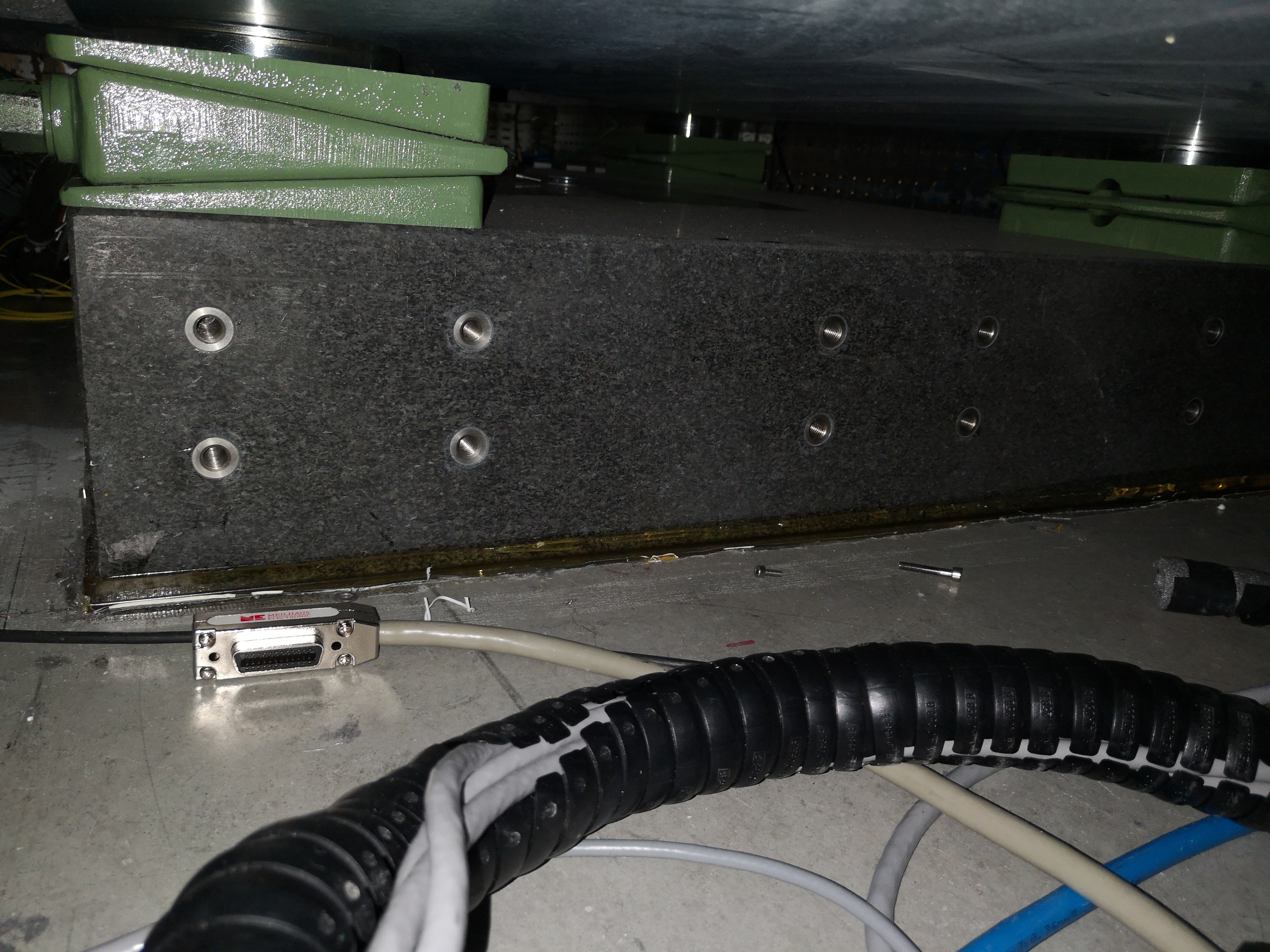
They are probably not well leveled, so the granite is supported only by two Airloc.
Setup
Mode extraction and importation
First, we split the big modes.asc files into sub text files using bash.
  sed '/^\s*[0-9]*[XYZ][+-]:/!d' modal_analysis_updated/modes.asc > mat/mode_shapes.txt
  sed '/freq/!d' modal_analysis_updated/modes.asc | sed 's/.* = \(.*\)Hz/\1/' > mat/mode_freqs.txt
  sed '/damp/!d' modal_analysis_updated/modes.asc | sed 's/.* = \(.*\)\%/\1/' > mat/mode_damps.txt
  sed '/modal A/!d' modal_analysis_updated/modes.asc | sed 's/.* =\s\+\([-0-9.e]\++[0-9]\+\)\([-+0-9.e]\+\)i/\1 \2/' > mat/mode_modal_a.txt
  sed '/modal B/!d' modal_analysis_updated/modes.asc | sed 's/.* =\s\+\([-0-9.e]\++[0-9]\+\)\([-+0-9.e]\+\)i/\1 \2/' > mat/mode_modal_b.txt
Then we import them on Matlab.
  shapes = readtable('mat/mode_shapes.txt', 'ReadVariableNames', false); % [Sign / Real / Imag]
  freqs = table2array(readtable('mat/mode_freqs.txt', 'ReadVariableNames', false)); % in [Hz]
  damps = table2array(readtable('mat/mode_damps.txt', 'ReadVariableNames', false)); % in [%]
  modal_a = table2array(readtable('mat/mode_modal_a.txt', 'ReadVariableNames', false)); % [Real / Imag]
  modal_a = complex(modal_a(:, 1), modal_a(:, 2));
  modal_b = table2array(readtable('mat/mode_modal_b.txt', 'ReadVariableNames', false)); % [Real / Imag]
  modal_b = complex(modal_b(:, 1), modal_b(:, 2));
We guess the number of modes identified from the length of the imported data.
  acc_n = 23; % Number of accelerometers
  dir_n = 3; % Number of directions
  dirs = 'XYZ';

  mod_n = size(shapes,1)/acc_n/dir_n; % Number of modes
As the mode shapes are split into 3 parts (direction plus sign, real part and imaginary part), we aggregate them into one array of complex numbers.
  T_sign = table2array(shapes(:, 1));
  T_real = table2array(shapes(:, 2));
  T_imag = table2array(shapes(:, 3));

  modes = zeros(mod_n, acc_n, dir_n);

  for mod_i = 1:mod_n
    for acc_i = 1:acc_n
      % Get the correct section of the signs
      T = T_sign(acc_n*dir_n*(mod_i-1)+1:acc_n*dir_n*mod_i);
      for dir_i = 1:dir_n
        % Get the line corresponding to the sensor
        i = find(contains(T, sprintf('%i%s',acc_i, dirs(dir_i))), 1, 'first')+acc_n*dir_n*(mod_i-1);
        modes(mod_i, acc_i, dir_i) = str2num([T_sign{i}(end-1), '1'])*complex(T_real(i),T_imag(i));
      end
    end
  end
The obtained mode frequencies and damping are shown below.
data2orgtable([freqs, damps], {}, {'Frequency [Hz]', 'Damping [%]'}, ' %.1f ');| Frequency [Hz] | Damping [%] |
|---|---|
| 11.4 | 8.7 |
| 18.5 | 11.8 |
| 37.6 | 6.4 |
| 39.4 | 3.6 |
| 54.0 | 0.2 |
| 56.1 | 2.8 |
| 69.7 | 4.6 |
| 71.6 | 0.6 |
| 72.4 | 1.6 |
| 84.9 | 3.6 |
| 90.6 | 0.3 |
| 91.0 | 2.9 |
| 95.8 | 3.3 |
| 105.4 | 3.3 |
| 106.8 | 1.9 |
| 112.6 | 3.0 |
| 116.8 | 2.7 |
| 124.1 | 0.6 |
| 145.4 | 1.6 |
| 150.1 | 2.2 |
| 164.7 | 1.4 |
Positions of the sensors
We process the file exported from the modal software containing the positions of the sensors using bash.
cat modal_analysis_updated/id31_nanostation_modified.cfg | grep NODES -A 23 | sed '/\s\+[0-9]\+/!d' | sed 's/\(.*\)\s\+0\s\+.\+/\1/' > mat/acc_pos.txt
We then import that on matlab, and sort them.
  acc_pos = readtable('mat/acc_pos.txt', 'ReadVariableNames', false);
  acc_pos = table2array(acc_pos(:, 1:4));
  [~, i] = sort(acc_pos(:, 1));
  acc_pos = acc_pos(i, 2:4);
The positions of the sensors relative to the point of interest are shown below.
data2orgtable(1000*acc_pos, {}, {'x [mm]', 'y [mm]', 'z [mm]'}, ' %.0f ');| x [mm] | y [mm] | z [mm] |
|---|---|---|
| -64 | -64 | -296 |
| -64 | 64 | -296 |
| 64 | 64 | -296 |
| 64 | -64 | -296 |
| -385 | -300 | -417 |
| -420 | 280 | -417 |
| 420 | 280 | -417 |
| 380 | -300 | -417 |
| -475 | -414 | -427 |
| -465 | 407 | -427 |
| 475 | 424 | -427 |
| 475 | -419 | -427 |
| -320 | -446 | -786 |
| -480 | 534 | -786 |
| 450 | 534 | -786 |
| 295 | -481 | -786 |
| -730 | -526 | -951 |
| -735 | 814 | -951 |
| 875 | 799 | -951 |
| 865 | -506 | -951 |
| -155 | -90 | -594 |
| 0 | 180 | -594 |
| 155 | -90 | -594 |
Solids
We consider the following solid bodies:
- Bottom Granite
- Top Granite
- Translation Stage
- Tilt Stage
- Spindle
- Hexapod
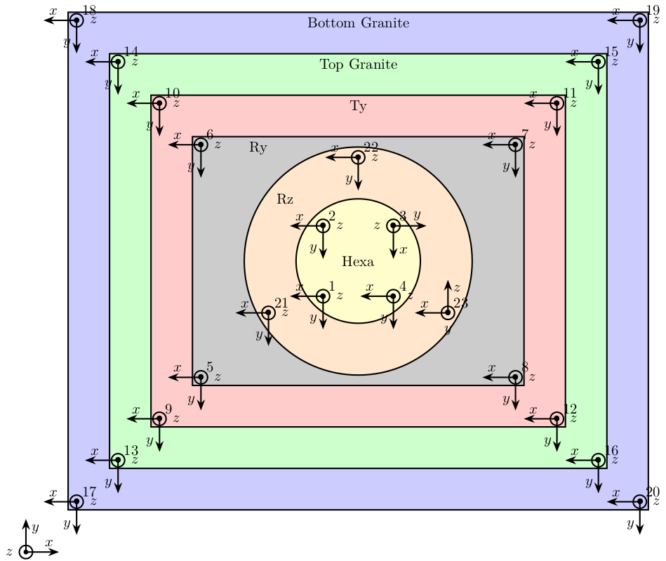
We create a structure solids that contains the accelerometer number of each solid bodies (as shown on figure fig:nass-modal-test).
  solids = {};
  solids.granite_bot = [17, 18, 19, 20];
  solids.granite_top = [13, 14, 15, 16];
  solids.ty          = [9, 10, 11, 12];
  solids.ry          = [5, 6, 7, 8];
  solids.rz          = [21, 22, 23];
  solids.hexa        = [1, 2, 3, 4];

  solid_names = fields(solids);
From local coordinates to global coordinates for the mode shapes
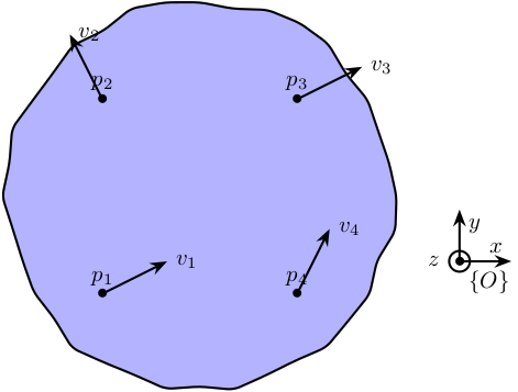
From the figure above, we can write:
\begin{align*} \vec{v}_1 &= \vec{v} + \Omega \vec{p}_1\\ \vec{v}_2 &= \vec{v} + \Omega \vec{p}_2\\ \vec{v}_3 &= \vec{v} + \Omega \vec{p}_3\\ \vec{v}_4 &= \vec{v} + \Omega \vec{p}_4 \end{align*}With
\begin{equation} \Omega = \begin{bmatrix} 0 & -\Omega_z & \Omega_y \\ \Omega_z & 0 & -\Omega_x \\ -\Omega_y & \Omega_x & 0 \end{bmatrix} \end{equation}$\vec{v}$ and $\Omega$ represent to velocity and rotation of the solid expressed in the frame $\{O\}$.
We can rearrange the equations in a matrix form:
\begin{equation} \left[\begin{array}{ccc|ccc} 1 & 0 & 0 & 0 & p_{1z} & -p_{1y} \\ 0 & 1 & 0 & -p_{1z} & 0 & p_{1x} \\ 0 & 0 & 1 & p_{1y} & -p_{1x} & 0 \\ \hline & \vdots & & & \vdots & \\ \hline 1 & 0 & 0 & 0 & p_{4z} & -p_{4y} \\ 0 & 1 & 0 & -p_{4z} & 0 & p_{4x} \\ 0 & 0 & 1 & p_{4y} & -p_{4x} & 0 \end{array}\right] \begin{bmatrix} v_x \\ v_y \\ v_z \\ \hline \Omega_x \\ \Omega_y \\ \Omega_z \end{bmatrix} = \begin{bmatrix} v_{1x} \\ v_{1y} \\ v_{1z} \\\hline \vdots \\\hline v_{4x} \\ v_{4y} \\ v_{4z} \end{bmatrix} \end{equation}and then we obtain the velocity and rotation of the solid in the wanted frame $\{O\}$:
\begin{equation} \begin{bmatrix} v_x \\ v_y \\ v_z \\ \hline \Omega_x \\ \Omega_y \\ \Omega_z \end{bmatrix} = \left[\begin{array}{ccc|ccc} 1 & 0 & 0 & 0 & p_{1z} & -p_{1y} \\ 0 & 1 & 0 & -p_{1z} & 0 & p_{1x} \\ 0 & 0 & 1 & p_{1y} & -p_{1x} & 0 \\ \hline & \vdots & & & \vdots & \\ \hline 1 & 0 & 0 & 0 & p_{4z} & -p_{4y} \\ 0 & 1 & 0 & -p_{4z} & 0 & p_{4x} \\ 0 & 0 & 1 & p_{4y} & -p_{4x} & 0 \end{array}\right]^{-1} \begin{bmatrix} v_{1x} \\ v_{1y} \\ v_{1z} \\\hline \vdots \\\hline v_{4x} \\ v_{4y} \\ v_{4z} \end{bmatrix} \end{equation}This inversion is equivalent to a mean square problem.
  mode_shapes_O = zeros(mod_n, length(solid_names), 6);

  for mod_i = 1:mod_n
    for solid_i = 1:length(solid_names)
      solids_i = solids.(solid_names{solid_i});

      Y = reshape(squeeze(modes(mod_i, solids_i, :))', [], 1);

      A = zeros(3*length(solids_i), 6);
      for i = 1:length(solids_i)
        A(3*(i-1)+1:3*i, 1:3) = eye(3);

        A(3*(i-1)+1:3*i, 4:6) = [0 acc_pos(i, 3) -acc_pos(i, 2) ; -acc_pos(i, 3) 0 acc_pos(i, 1) ; acc_pos(i, 2) -acc_pos(i, 1) 0];
      end

      mode_shapes_O(mod_i, solid_i, :) = A\Y;
    end
  end
Modal Matrices
We want to obtain the two following matrices: \[ \Omega = \begin{bmatrix} \omega_1^2 & & 0 \\ & \ddots & \\ 0 & & \omega_n^2 \end{bmatrix}; \quad \Psi = \begin{bmatrix} & & \\ \{\psi_1\} & \dots & \{\psi_n\} \\ & & \end{bmatrix} \]
- How to add damping to the eigen value matrix?
  eigen_value_M = diag(freqs*2*pi);
  eigen_vector_M = reshape(mode_shapes_O, [mod_n, 6*length(solid_names)])';
\[ \{\psi_1\} = \begin{Bmatrix} \psi_{1_x} & \psi_{2_x} & \dots & \psi_{6_x} & \psi_{1_x} & \dots & \psi_{1\Omega_x} & \dots & \psi_{6\Omega_z} \end{Bmatrix}^T \]
Modal Complexity
A method of displaying modal complexity is by plotting the elements of the eigenvector on an Argand diagram, such as the ones shown in figure fig:modal_complexity_small.
To evaluate the complexity of the modes, we plot a polygon around the extremities of the individual vectors. The obtained area of this polygon is then compared with the area of the circle which is based on the length of the largest vector element. The resulting ratio is used as an indication of the complexity of the mode.
A little complex mode is shown on figure fig:modal_complexity_small whereas an highly complex mode is shown on figure fig:modal_complexity_high. The complexity of all the modes are compared on figure fig:modal_complexities.
<<plt-matlab>>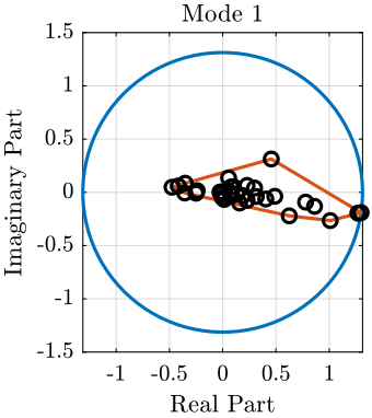
<<plt-matlab>>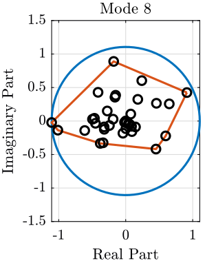
<<plt-matlab>>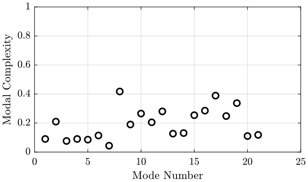
Some notes about constraining the number of degrees of freedom
We want to have the two eigen matrices.
They should have the same size $n \times n$ where $n$ is the number of modes as well as the number of degrees of freedom. Thus, if we consider 21 modes, we should restrict our system to have only 21 DOFs.
Actually, we are measured 6 DOFs of 6 solids, thus we have 36 DOFs.
From the mode shapes animations, it seems that in the frequency range of interest, the two marbles can be considered as one solid. We thus have 5 solids and 30 DOFs.
In order to determine which DOF can be neglected, two solutions seems possible:
- compare the mode shapes
- compare the FRFs
The question is: in which base (frame) should be express the modes shapes and FRFs? Is it meaningful to compare mode shapes as they give no information about the amplitudes of vibration?
| Stage | Motion DOFs | Parasitic DOF | Total DOF | Description of DOF |
|---|---|---|---|---|
| Granite | 0 | 3 | 3 | |
| Ty | 1 | 2 | 3 | Ty, Rz |
| Ry | 1 | 2 | 3 | Ry, |
| Rz | 1 | 2 | 3 | Rz, Rx, Ry |
| Hexapod | 6 | 0 | 6 | Txyz, Rxyz |
| 9 | 9 | 18 |
TODO Normalization of mode shapes?
We normalize each column of the eigen vector matrix. Then, each eigenvector as a norm of 1.
eigen_vector_M = eigen_vector_M./vecnorm(eigen_vector_M);Compare Mode Shapes
Let's say we want to see for the first mode which DOFs can be neglected. In order to do so, we should estimate the motion of each stage in particular directions. If we look at the z motion for instance, we will find that we cannot neglect that motion (because of the tilt causing z motion).
  mode_i = 3;
  dof_i = 6;

  mode = eigen_vector_M(dof_i:6:end, mode_i);

  figure;
  hold on;
  for i=1:length(mode)
    plot([0, real(mode(i))], [0, imag(mode(i))], '-', 'DisplayName', solid_names{i});
  end
  hold off;
legend(); figure;
subplot(2, 1, 1);
hold on;
for i=1:length(mode)
plot(1, norm(mode(i)), 'o');
end
hold off;
ylabel('Amplitude');
subplot(2, 1, 2);
hold on;
for i=1:length(mode)
plot(1, 180/pi*angle(mode(i)), 'o', 'DisplayName', solid_names{i});
end
hold off;
ylim([-180, 180]); yticks([-180:90:180]);
ylabel('Phase [deg]');
legend(); test = mode_shapes_O(10, 1, :)/norm(squeeze(mode_shapes_O(10, 1, :)));
test = mode_shapes_O(10, 2, :)/norm(squeeze(mode_shapes_O(10, 2, :)));Importation of measured FRF curves
There are 24 measurements files corresponding to 24 series of impacts:
- 3 directions, 8 sets of 3 accelerometers
For each measurement file, the FRF and coherence between the impact and the 9 accelerations measured.
In reality: 4 sets of 10 things
a = load('mat/meas_frf_coh_1.mat'); figure;
ax1 = subplot(2, 1, 1);
hold on;
plot(a.FFT1_AvXSpc_2_1_RMS_X_Val, a.FFT1_AvXSpc_2_1_RMS_Y_Mod)
hold off;
set(gca, 'XScale', 'log'); set(gca, 'YScale', 'log');
set(gca, 'XTickLabel',[]);
ylabel('Amplitude');
title(sprintf('From %s, to %s', FFT1_AvXSpc_2_1_RfName, FFT1_AvXSpc_2_1_RpName))
ax2 = subplot(2, 1, 2);
hold on;
plot(a.FFT1_AvXSpc_2_1_RMS_X_Val, a.FFT1_AvXSpc_2_1_RMS_Y_Phas)
hold off;
ylim([-180, 180]); yticks(-180:90:180);
xlabel('Frequency [Hz]'); ylabel('Phase [deg]');
set(gca, 'xscale', 'log');
linkaxes([ax1,ax2],'x');
xlim([1, 200]);Importation of measured FRF curves to global FRF matrix
FRF matrix $n \times p$:
- $n$ is the number of measurements: $3 \times 24$
- $p$ is the number of excitation inputs: 3
23 measurements: 3 accelerometers
\begin{equation} \text{FRF}(\omega_i) = \begin{bmatrix} \frac{D_{1_x}}{F_x}(\omega_i) & \frac{D_{1_x}}{F_y}(\omega_i) & \frac{D_{1_x}}{F_z}(\omega_i) \\ \frac{D_{1_y}}{F_x}(\omega_i) & \frac{D_{1_y}}{F_y}(\omega_i) & \frac{D_{1_y}}{F_z}(\omega_i) \\ \frac{D_{1_z}}{F_x}(\omega_i) & \frac{D_{1_z}}{F_y}(\omega_i) & \frac{D_{1_z}}{F_z}(\omega_i) \\ \frac{D_{2_x}}{F_x}(\omega_i) & \frac{D_{2_x}}{F_y}(\omega_i) & \frac{D_{2_x}}{F_z}(\omega_i) \\ \vdots & \vdots & \vdots \\ \frac{D_{23_z}}{F_x}(\omega_i) & \frac{D_{23_z}}{F_y}(\omega_i) & \frac{D_{23_z}}{F_z}(\omega_i) \\ \end{bmatrix} \end{equation} n_meas = 24;
n_acc = 23;
dirs = 'XYZ';
% Number of Accelerometer * DOF for each acccelerometer / Number of excitation / frequency points
FRFs = zeros(3*n_acc, 3, 801);
COHs = zeros(3*n_acc, 3, 801);
% Loop through measurements
for i = 1:n_meas
% Load the measurement file
meas = load(sprintf('mat/meas_frf_coh_%i.mat', i));
% First: determine what is the exitation (direction and sign)
exc_dir = meas.FFT1_AvXSpc_2_1_RMS_RfName(end);
exc_sign = meas.FFT1_AvXSpc_2_1_RMS_RfName(end-1);
% Determine what is the correct excitation sign
exc_factor = str2num([exc_sign, '1']);
if exc_dir ~= 'Z'
exc_factor = exc_factor*(-1);
end
% Then: loop through the nine measurements and store them at the correct location
for j = 2:10
% Determine what is the accelerometer and direction
[indices_acc_i] = strfind(meas.(sprintf('FFT1_H1_%i_1_RpName', j)), '.');
acc_i = str2num(meas.(sprintf('FFT1_H1_%i_1_RpName', j))(indices_acc_i(1)+1:indices_acc_i(2)-1));
meas_dir = meas.(sprintf('FFT1_H1_%i_1_RpName', j))(end);
meas_sign = meas.(sprintf('FFT1_H1_%i_1_RpName', j))(end-1);
% Determine what is the correct measurement sign
meas_factor = str2num([meas_sign, '1']);
if meas_dir ~= 'Z'
meas_factor = meas_factor*(-1);
end
% FRFs(acc_i+n_acc*(find(dirs==meas_dir)-1), find(dirs==exc_dir), :) = exc_factor*meas_factor*meas.(sprintf('FFT1_H1_%i_1_Y_ReIm', j));
% COHs(acc_i+n_acc*(find(dirs==meas_dir)-1), find(dirs==exc_dir), :) = meas.(sprintf('FFT1_Coh_%i_1_RMS_Y_Val', j));
FRFs(find(dirs==meas_dir)+3*(acc_i-1), find(dirs==exc_dir), :) = exc_factor*meas_factor*meas.(sprintf('FFT1_H1_%i_1_Y_ReIm', j));
COHs(find(dirs==meas_dir)+3*(acc_i-1), find(dirs==exc_dir), :) = meas.(sprintf('FFT1_Coh_%i_1_RMS_Y_Val', j));
end
end
freqs = meas.FFT1_Coh_10_1_RMS_X_Val;Analysis of some FRFs
  acc_i = 3;
  acc_dir = 1;
  exc_dir = 1;

  figure;

  ax1 = subplot(2, 1, 1);
  hold on;
  plot(freqs, abs(squeeze(FRFs(acc_dir+3*(acc_i-1), exc_dir, :))));
  hold off;
  set(gca, 'XScale', 'log'); set(gca, 'YScale', 'log');
  set(gca, 'XTickLabel',[]);
  ylabel('Amplitude');

  ax2 = subplot(2, 1, 2);
  hold on;
  plot(freqs, mod(180+180/pi*phase(squeeze(FRFs(acc_dir+3*(acc_i-1), exc_dir, :))), 360)-180);
  hold off;
  ylim([-180, 180]); yticks(-180:90:180);
  xlabel('Frequency [Hz]'); ylabel('Phase [deg]');
  set(gca, 'xscale', 'log');

  linkaxes([ax1,ax2],'x');
  xlim([1, 200]);
Composite Response Function
We here sum the norm instead of the complex numbers.
  HHx = squeeze(sum(abs(FRFs(:, 1, :))));
  HHy = squeeze(sum(abs(FRFs(:, 2, :))));
  HHz = squeeze(sum(abs(FRFs(:, 3, :))));
  HH  = squeeze(sum([HHx, HHy, HHz], 2));
exc_dir = 3;
figure;
hold on;
for i = 1:3*n_acc
plot(freqs, abs(squeeze(FRFs(i, exc_dir, :))), 'color', [0, 0, 0, 0.2]);
end
plot(freqs, abs(HHx));
plot(freqs, abs(HHy));
plot(freqs, abs(HHz));
plot(freqs, abs(HH), 'k');
hold off;
set(gca, 'XScale', 'lin'); set(gca, 'YScale', 'lin');
xlabel('Frequency [Hz]'); ylabel('Amplitude');
xlim([1, 200]); <<plt-matlab>>
TODO Singular Value Decomposition - Modal Indication Function
Show the same plot as in the modal software. This helps to identify double modes.
From the documentation of the modal software:
The MIF consist of the singular values of the Frequency response function matrix. The number of MIFs equals the number of excitations. By the powerful singular value decomposition, the real signal space is separated from the noise space. Therefore, the MIFs exhibit the modes effectively. A peak in the MIFs plot usually indicate the existence of a structural mode, and two peaks at the same frequency point means the existence of two repeated modes. Moreover, the magnitude of the MIFs implies the strength of the a mode.
From local coordinates to global coordinates with the FRFs
  % Number of Solids * DOF for each solid / Number of excitation / frequency points
  FRFs_O = zeros(length(solid_names)*6, 3, 801);

  for exc_dir = 1:3
    for solid_i = 1:length(solid_names)
      solids_i = solids.(solid_names{solid_i});

      A = zeros(3*length(solids_i), 6);
      for i = 1:length(solids_i)
        A(3*(i-1)+1:3*i, 1:3) = eye(3);

        A(3*(i-1)+1:3*i, 4:6) = [0 acc_pos(i, 3) -acc_pos(i, 2) ; -acc_pos(i, 3) 0 acc_pos(i, 1) ; acc_pos(i, 2) -acc_pos(i, 1) 0];
      end

      for i = 1:801
        FRFs_O((solid_i-1)*6+1:solid_i*6, exc_dir, i) = A\FRFs((solids_i(1)-1)*3+1:solids_i(end)*3, exc_dir, i);
      end
    end
  end
Analysis of some FRF in the global coordinates
  solid_i = 6;
  dir_i = 1;
  exc_dir = 1;

  figure;

  ax1 = subplot(2, 1, 1);
  hold on;
  plot(freqs, abs(squeeze(FRFs_O((solid_i-1)*6+dir_i, exc_dir, :))));
  hold off;
  set(gca, 'XScale', 'log'); set(gca, 'YScale', 'log');
  set(gca, 'XTickLabel',[]);
  ylabel('Amplitude');

  ax2 = subplot(2, 1, 2);
  hold on;
  plot(freqs, mod(180+180/pi*phase(squeeze(FRFs_O((solid_i-1)*6+dir_i, exc_dir, :))), 360)-180);
  hold off;
  ylim([-180, 180]); yticks(-180:90:180);
  xlabel('Frequency [Hz]'); ylabel('Phase [deg]');
  set(gca, 'xscale', 'log');

  linkaxes([ax1,ax2],'x');
  xlim([1, 200]);
Compare global coordinates to local coordinates
  solid_i = 1;
  acc_dir_O = 6;
  acc_dir = 3;
  exc_dir = 3;

  figure;

  ax1 = subplot(2, 1, 1);
  hold on;
  for i = solids.(solid_names{solid_i})
    plot(freqs, abs(squeeze(FRFs(acc_dir+3*(i-1), exc_dir, :))));
  end
  plot(freqs, abs(squeeze(FRFs_O((solid_i-1)*6+acc_dir_O, exc_dir, :))), '-k');
  hold off;
  set(gca, 'XScale', 'log'); set(gca, 'YScale', 'log');
  set(gca, 'XTickLabel',[]);
  ylabel('Amplitude');

  ax2 = subplot(2, 1, 2);
  hold on;
  for i = solids.(solid_names{solid_i})
    plot(freqs, mod(180+180/pi*phase(squeeze(FRFs(acc_dir+3*(i-1), exc_dir, :))), 360)-180);
  end
  plot(freqs, mod(180+180/pi*phase(squeeze(FRFs_O((solid_i-1)*6+acc_dir_O, exc_dir, :))), 360)-180, '-k');
  hold off;
  ylim([-180, 180]); yticks(-180:90:180);
  xlabel('Frequency [Hz]'); ylabel('Phase [deg]');
  set(gca, 'xscale', 'log');

  linkaxes([ax1,ax2],'x');
  xlim([1, 200]);
Verify that we find the original FRF from the FRF in the global coordinates
From the computed FRF of the Hexapod in its 6 DOFs, compute the FRF of the accelerometer 1 fixed to the Hexapod during the measurement.
  FRF_test = zeros(801, 3);
  for i = 1:801
    FRF_test(i, :) = FRFs_O(31:33, 1, i) + cross(FRFs_O(34:36, 1, i), acc_pos(1, :)');
end <<plt-matlab>>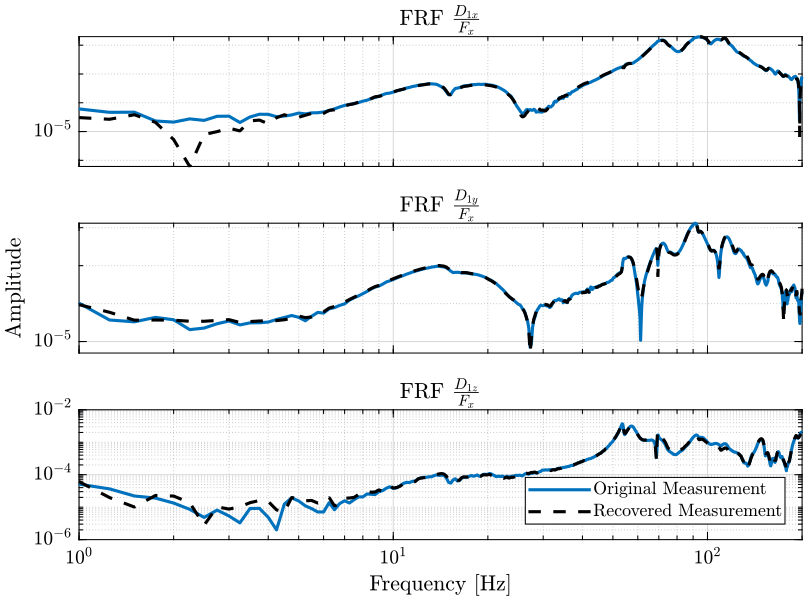
The reduction of the number of degrees of freedom from 69 (23 accelerometers with each 3DOF) to 36 (6 solid bodies with 6 DOF) seems to work well.
This confirms the fact that this stage, for that mode is indeed behaving as a solid body. This should be verified for all the stages for modes with high resonance frequencies.