nass-micro-station-measurements/huddle-test-geophones/index.org

• Setup
• Signal Processing
  • Load data
  • Time Domain Data
  • Compute PSD
  • Take into account sensibility of Geophone
  • Transfer function between the two geophones

#+TITLE:SpeedGoat

Setup

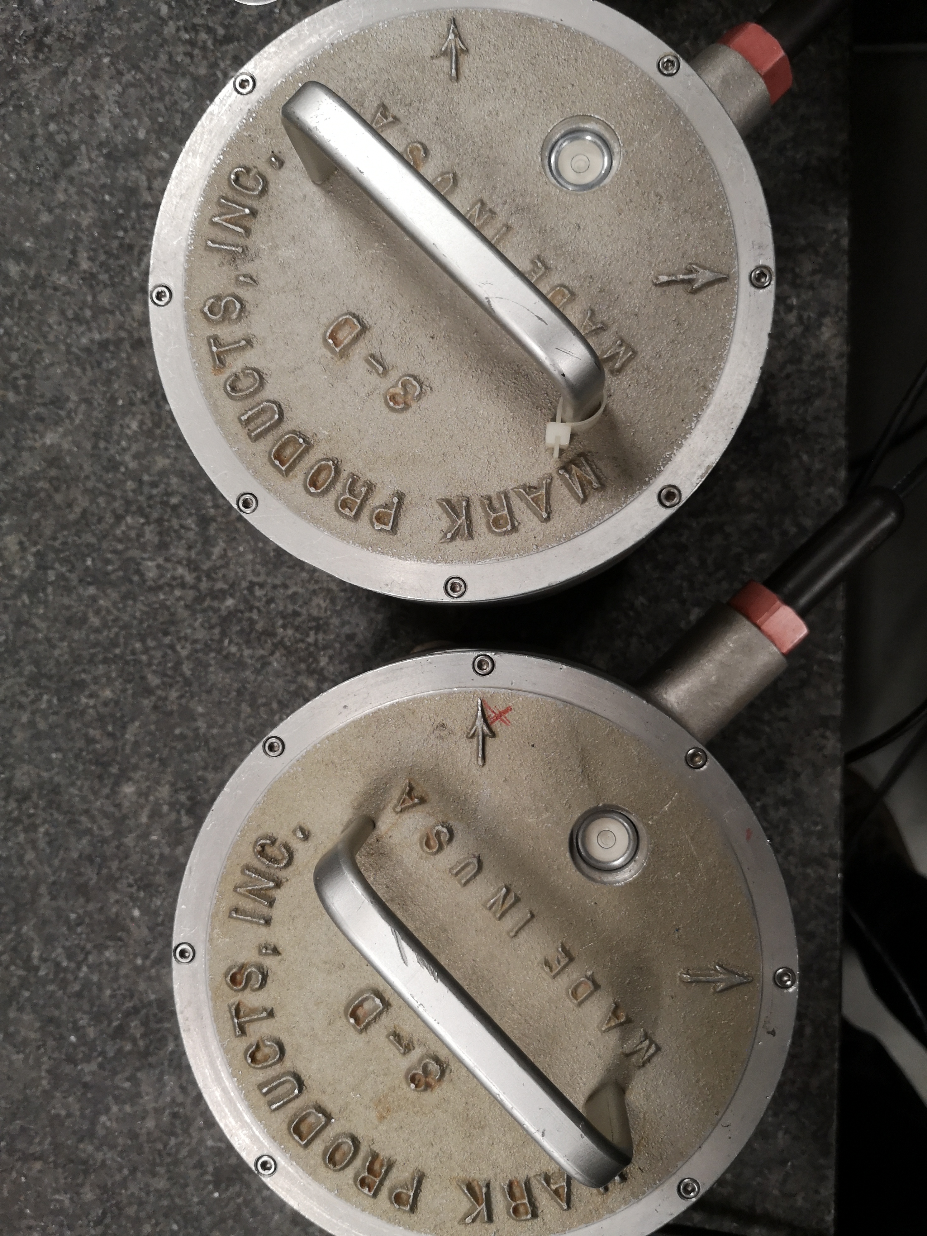
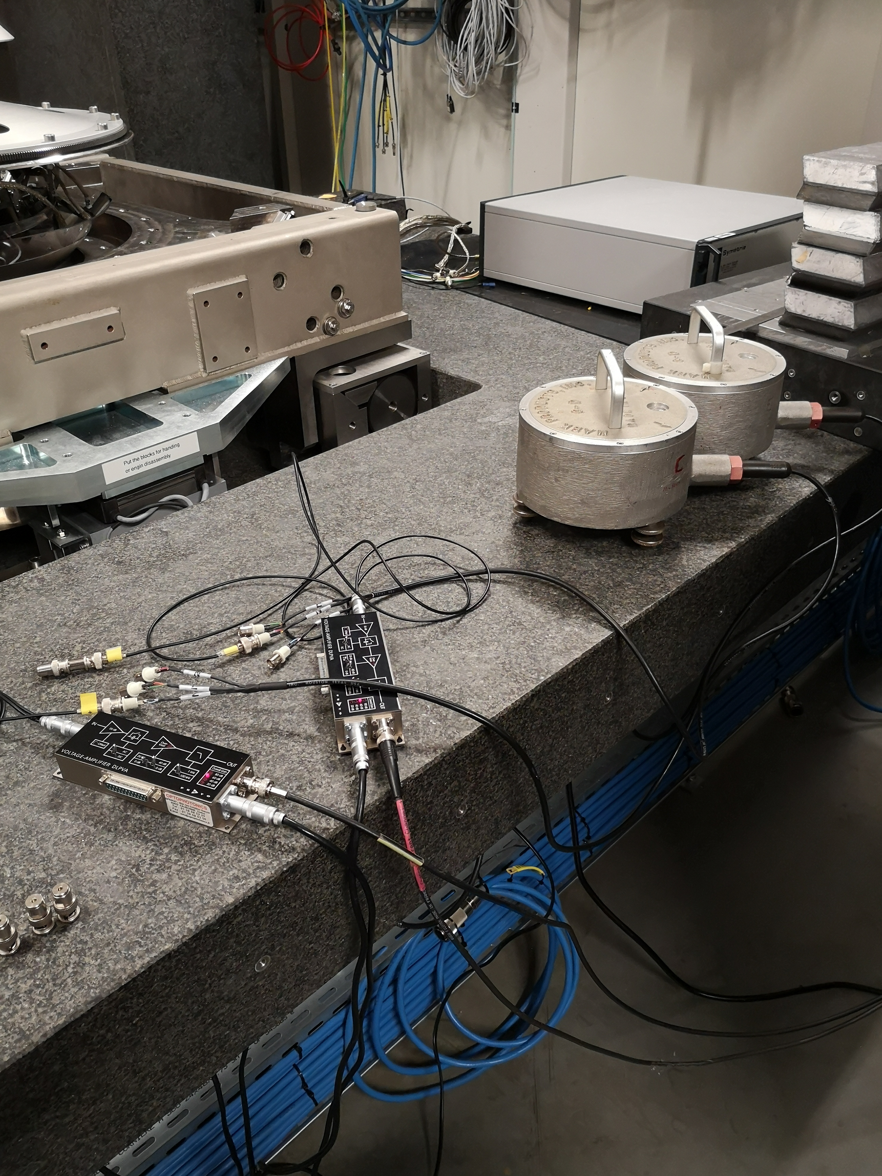
Two L22 geophones are used. They are placed on the ID31 granite. They are leveled.

The signals are amplified using voltage amplifier with a gain of 60dB. The voltage amplifiers include a low pass filter with a cut-off frequency at 1kHz.

Setup

Geophones

Signal Processing

Load data

  load('mat/data_001.mat', 't', 'x1', 'x2');
  dt = t(2) - t(1);

Time Domain Data

  figure;
  hold on;
  plot(t, x1);
  plot(t, x2);
  hold off;
  xlabel('Time [s]');
  ylabel('Voltage [V]');
  xlim([t(1), t(end)]);

  <<plt-matlab>>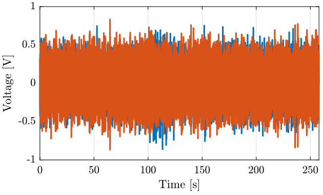

Time domain Data

  figure;
  hold on;
  plot(t, x1);
  plot(t, x2);
  hold off;
  xlabel('Time [s]');
  ylabel('Voltage [V]');
  xlim([0 1]);

  <<plt-matlab>>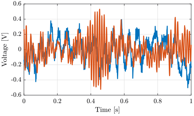

Time domain Data - Zoom

Compute PSD

  [pxx1, f1] = pwelch(x1, hanning(ceil(1/dt)), 0, [], 1/dt);
  [pxx2, f2] = pwelch(x2, hanning(ceil(1/dt)), 0, [], 1/dt);

Take into account sensibility of Geophone

The Geophone used are L22.

  S0 = 88; % Sensitivity [V/(m/s)]
  f0 = 2; % Cut-off frequnecy [Hz]
  S = (s/2/pi/f0)/(1+s/2/pi/f0);

  figure;
  bodeFig({S});
  ylabel('Amplitude [V/(m/s)]')

  <<plt-matlab>>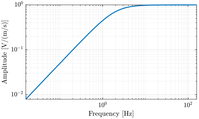

Sensibility of the Geophone

We take into account the gain of the electronics. The cut-off frequency is set at 1kHz.

• Check what is the order of the filter
• Maybe I should not use this filter as there is no high frequencies anyway?

  G0 = 60; % [dB]

  G = G0/(1+s/2/pi/1000);

  figure;
  hold on;
  plot(f1, sqrt(pxx1)./squeeze(abs(freqresp(G, f1, 'Hz')))./squeeze(abs(freqresp(S, f1, 'Hz'))));
  plot(f2, sqrt(pxx2)./squeeze(abs(freqresp(G, f2, 'Hz')))./squeeze(abs(freqresp(S, f2, 'Hz'))));
  hold off;
  set(gca, 'xscale', 'log');
  set(gca, 'yscale', 'log');
  xlabel('Frequency [Hz]'); ylabel('PSD [m/s/sqrt(Hz)]')
  xlim([2, 500]);

  <<plt-matlab>>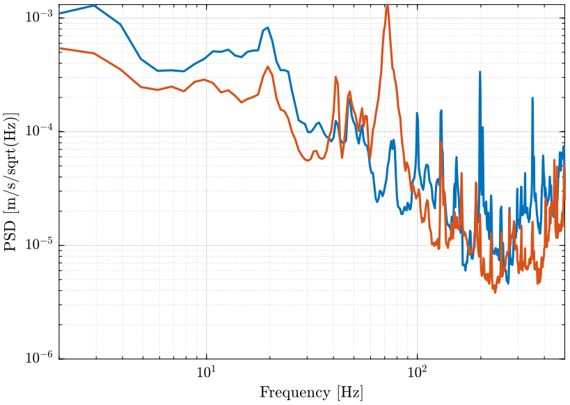

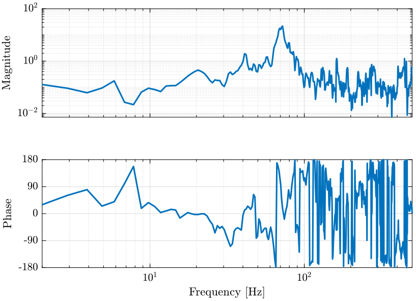
Spectral density of the velocity

Transfer function between the two geophones

  [T12, f12] = tfestimate(x1, x2, hanning(1/dt), 0, [], 1/dt);

  figure;
  ax1 = subplot(2, 1, 1);
  plot(f12, abs(T12));
  set(gca, 'xscale', 'log'); set(gca, 'yscale', 'log');
  set(gca, 'XTickLabel',[]);
  ylabel('Magnitude');

  ax2 = subplot(2, 1, 2);
  plot(f12, mod(180+180/pi*phase(T12), 360)-180);
  set(gca, 'xscale', 'log');
  ylim([-180, 180]);
  yticks([-180, -90, 0, 90, 180]);
  xlabel('Frequency [Hz]'); ylabel('Phase');

  linkaxes([ax1,ax2],'x');
  xlim([2, 500]);

  <<plt-matlab>>

Estimated transfer function between the two geophones