nass-metrology-test-bench/index.org

Cercalo Test Bench

• Introduction
  • Block Diagram
  • Cercalo
  • Optical Setup
  • Newport
  • 4 quadrant Diode
  • ADC/DAC
• Identification of the system dynamics
  • Introduction
  • ZIP file containing the data and matlab files
  • Calibration of the 4 Quadrant Diode
    • Introduction
    • Input / Output data
    • Linear Regression to obtain the gain of the 4QD
  • Identification of the Cercalo Impedance, Current Amplifier and Voltage Amplifier dynamics
    • Introduction
    • Electrical Schematic
    • Theoretical Transfer Functions
    • Identified Transfer Functions
  • Identification of the Cercalo Dynamics
    • Introduction
    • Input / Output data
    • Coherence
    • Estimation of the Frequency Response Function Matrix
    • Time Delay
    • Extraction of a transfer function matrix
  • Identification of the Newport Dynamics
    • Introduction
    • Input / Output data
    • Coherence
    • Estimation of the Frequency Response Function Matrix
    • Time Delay
    • Extraction of a transfer function matrix
  • Full System
• Active Damping
  • Load Plant
  • Test
• Huddle Test
• Plant Scaling
  • General Configuration
• Plant Analysis
  • Load Plant
  • RGA-Number
  • Rotation Matrix
• Control Objective
• Decentralized Control
  • Introduction
  • ZIP file containing the data and matlab files
  • Load Plant
  • Diagonal Controller
  • Save the Controller
• Newport Control
  • Introduction
  • Load Plant
  • Analysis
  • Save
• Measurement of the non-repeatability
  • Data Load
  • Some Plots
  • Repeatability

Introduction

Block Diagram

The block diagram of the setup to be controlled is shown in Fig. fig:block_diagram_simplify.

Block Diagram of the Experimental Setup

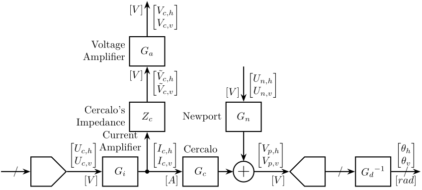
The transfer functions in the system are:

• Current Amplifier: from the voltage set by the DAC to the current going to the Cercalo's inductors \[ G_i = \begin{bmatrix} G_{i,h} & 0 \\ 0 & G_{i,v} \end{bmatrix} \text{ in } \left[ \frac{A}{V} \right] \] \[ \begin{bmatrix} I_{c,h} \\ I_{c,v} \end{bmatrix} = G_i \begin{bmatrix} U_{c,h} \\ U_{c,v} \end{bmatrix} \]
• Impedance of the Cercalo that converts the current going to the cercalo to the voltage across the cercalo: \[ Z_c = \begin{bmatrix} Z_{c,h} & 0 \\ 0 & Z_{c,v} \end{bmatrix} \text{ in } \left[ \frac{V}{A} \right] \] \[ \begin{bmatrix} \tilde{V}_{c,h} \\ \tilde{V}_{c,v} \end{bmatrix} = Z_c \begin{bmatrix} I_{c,h} \\ I_{c,v} \end{bmatrix} \]
• Voltage Amplifier: from the voltage across the Cercalo inductors to the measured voltage \[ G_a = \begin{bmatrix} G_{a,h} & 0 \\ 0 & G_{a,v} \end{bmatrix} \text{ in } \left[ \frac{V}{V} \right] \] \[ \begin{bmatrix} V_{c,h} \\ V_{c,v} \end{bmatrix} = G_a \begin{bmatrix} \tilde{V}_{c,h} \\ \tilde{V}_{c,v} \end{bmatrix} \]
• Cercalo: Transfer function from the current going through the cercalo inductors to the 4 quadrant measurement \[ G_c = \begin{bmatrix} G_{\frac{V_{p,h}}{\tilde{U}_{c,h}}} & G_{\frac{V_{p,h}}{\tilde{U}_{c,v}}} \\ G_{\frac{V_{p,v}}{\tilde{U}_{c,h}}} & G_{\frac{V_{p,v}}{\tilde{U}_{c,v}}} \end{bmatrix} \text{ in } \left[ \frac{V}{A} \right] \] \[ \begin{bmatrix} V_{p,h} \\ V_{p,v} \end{bmatrix} = G_c \begin{bmatrix} I_{c,h} \\ I_{c,v} \end{bmatrix} \]
• Newport Transfer function from the command signal of the Newport to the 4 quadrant measurement \[ G_n = \begin{bmatrix} G_{\frac{V_{p,h}}{U_{n,h}}} & G_{\frac{V_{p,h}}{U_{n,v}}} \\ G_{\frac{V_{p,v}}{U_{n,h}}} & G_{\frac{V_{n,v}}{U_{n,v}}} \end{bmatrix} \text{ in } \left[ \frac{V}{V} \right] \] \[ \begin{bmatrix} V_{p,h} \\ V_{p,v} \end{bmatrix} = G_c \begin{bmatrix} V_{n,h} \\ V_{n,v} \end{bmatrix} \]
• 4 Quadrant Diode: the gain of the 4 quadrant diode in [V/rad] is inverse in order to obtain the physical angle of the beam \[ G_d = \begin{bmatrix} G_{d,h} & 0 \\ 0 & G_{d,v} \end{bmatrix} \text{ in } \left[\frac{V}{rad}\right] \]

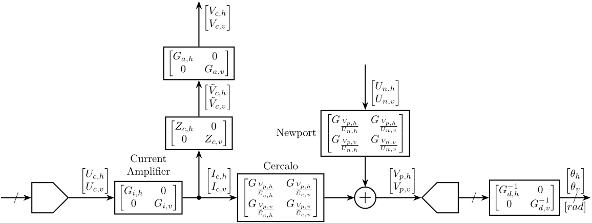
The block diagram with each transfer function is shown in Fig. fig:block_diagram.

Block Diagram of the Experimental Setup with detailed dynamics

Cercalo

From the Cercalo documentation, we have the parameters shown on table tab:cercalo_parameters.

	Maximum Stroke [deg]	Resonance Frequency [Hz]	DC Gain [mA/deg]	Gain at resonance [deg/V]	RC Resistance [Ohm]
AX1 (Horizontal)	5	411.13	28.4	382.9	9.41
AX2 (Vertical)	5	252.5	35.2	350.4

Cercalo Parameters

The Inductance and DC resistance of the two axis of the Cercalo have been measured:

• $L_{c,h} = 0.1\ \text{mH}$
• $L_{c,v} = 0.1\ \text{mH}$
• $R_{c,h} = 9.3\ \Omega$
• $R_{c,v} = 8.3\ \Omega$

Let's first consider the horizontal direction and we try to model the Cercalo by a spring/mass/damper system (Fig. fig:mech_cercalo).

1 degree-of-freedom model of the Cercalo

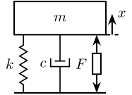
The equation of motion is:

\begin{align*} \frac{x}{F} &= \frac{1}{k + c s + m s^2} \\ &= \frac{G_0}{1 + 2 \xi \frac{s}{\omega_0} + \frac{s^2}{\omega_0^2}} \end{align*}

with:

• $G_0 = 1/k$ is the gain at DC in rad/N
• $\xi = \frac{c}{2 \sqrt{km}}$ is the damping ratio of the system
• $\omega_0 = \sqrt{\frac{k}{m}}$ is the resonance frequency in rad

The force $F$ applied to the mass is proportional to the current $I$ flowing through the voice coils: \[ \frac{F}{I} = \alpha \] with $\alpha$ is in $N/A$ and is to be determined.

The current $I$ is also proportional to the voltage at the output of the buffer:

\begin{align*} \frac{I_c}{U_c} &= \frac{1}{(R + R_c) + L_c s} \\ &\approx 0.02 \left[ \frac{A}{V} \right] \end{align*}

Let's try to determine the equivalent mass and spring values. From table tab:cercalo_parameters, for the horizontal direction: \[ \left| \frac{x}{I} \right|(0) = \left| \alpha \frac{x}{F} \right|(0) = 28.4\ \frac{mA}{deg} = 1.63\ \frac{A}{rad} \]

So: \[ \alpha \frac{1}{k} = 1.63 \Longleftrightarrow k = \frac{\alpha}{1.63} \left[\frac{N}{rad}\right] \]

We also know the resonance frequency: \[ \omega_0 = 411.1\ \text{Hz} = 2583\ \frac{rad}{s} \]

And the gain at resonance:

\begin{align*} \left| \frac{x}{U_c} \right|(j\omega_0) &= \left| 0.02 \frac{x}{I_c} \right| (j\omega_0) \\ &= \left| 0.02 \alpha \frac{x}{F} \right| (j\omega_0) \\ &= 0.02 \alpha \frac{1/k}{2\xi} \\ &= 282.9\ \left[\frac{deg}{V}\right] \\ &= 4.938\ \left[\frac{rad}{V}\right] \end{align*}

Thus:

\begin{align*} & \frac{\alpha}{2 \xi k} = 245 \\ \Leftrightarrow & \frac{1.63}{2 \xi} = 245 \\ \Leftrightarrow & \xi = 0.0033 \\ \Leftrightarrow & \xi = 0.33 \% \end{align*}

\begin{align*} G_0 &= \frac{1.63}{\alpha}\ \frac{rad}{N} \\ \xi &= 0.0033 \\ \omega_0 &= 2583\ \frac{rad}{s} \end{align*}

and in terms of the physical properties:

\begin{align*} k &= \frac{\alpha}{1.63}\ \frac{N}{rad} \\ \xi &= 0.0033 \\ m &= \frac{\alpha}{1.1 \cdot 10^7}\ \frac{kg}{m^2} \end{align*}

Thus, we have to determine $\alpha$. This can be done experimentally by determining the gain at DC or at resonance of the system. For that, we need to know the angle of the mirror, thus we need to calibrate the photo-diodes. This will be done using the Newport.

Optical Setup

Newport

Parameters of the Newport are shown in Fig. fig:newport_doc.

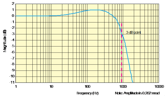
It's dynamics for small angle excitation is shown in Fig. fig:newport_gain.

And we have:

\begin{align*} G_{n, h}(0) &= 2.62 \cdot 10^{-3}\ \frac{rad}{V} \\ G_{n, v}(0) &= 2.62 \cdot 10^{-3}\ \frac{rad}{V} \end{align*}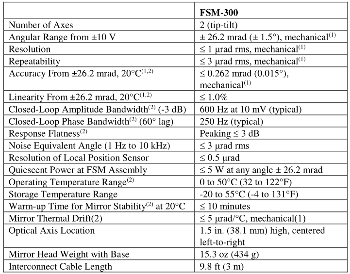

Documentation of the Newport

Transfer function of the Newport

4 quadrant Diode

The front view of the 4 quadrant photo-diode is shown in Fig. fig:4qd_naming.

Front view of the 4QD

Each of the photo-diode is amplified using a 4-channel amplifier as shown in Fig. fig:4qd_amplifier.

Wiring of the amplifier. The amplifier is located on the bottom right of the board

ADC/DAC

Let's compute the theoretical noise of the ADC/DAC.

\begin{align*} \Delta V &= 20 V \\ n &= 16bits \\ q &= \Delta V/2^n = 305 \mu V \\ f_N &= 10kHz \\ \Gamma_n &= \frac{q^2}{12 f_N} = 7.76 \cdot 10^{-13} \frac{V^2}{Hz} \end{align*}

with $\Delta V$ the total range of the ADC, $n$ its number of bits, $q$ the quantization, $f_N$ the sampling frequency and $\Gamma_n$ its theoretical Power Spectral Density.

Identification of the system dynamics

<<sec:cercalo_identification>>

Introduction   ignore

In this section, we seek to identify all the blocks as shown in Fig. fig:block_diagram_simplify.

Signal	Name	Unit
Voltage Sent to Cercalo - Horizontal	Uch	[V]
Voltage Sent to Cercalo - Vertical	Ucv	[V]
Voltage Sent to Newport - Horizontal	Unh	[V]
Voltage Sent to Newport - Vertical	Unv	[V]
4Q Photodiode Measurement - Horizontal	Vph	[V]
4Q Photodiode Measurement - Vertical	Vpv	[V]
Measured Voltage across the Inductance - Horizontal	Vch	[V]
Measured Voltage across the Inductance - Vertical	Vcv	[V]
Newport Metrology - Horizontal	Vnh	[V]
Newport Metrology - Vertical	Vnv	[V]
Attocube Measurement	Va	[m]

ZIP file containing the data and matlab files   ignore

All the files (data and Matlab scripts) are accessible here.

Calibration of the 4 Quadrant Diode

Introduction   ignore

Prior to any dynamic identification, we would like to be able to determine the meaning of the 4 quadrant diode measurement. For instance, instead of obtaining transfer function in [V/V] from the input of the cercalo to the measurement voltage of the 4QD, we would like to obtain the transfer function in [rad/V]. This will give insight to physical interpretation.

To calibrate the 4 quadrant photo-diode, we can use the metrology included in the Newport. We can choose precisely the angle of the Newport mirror and see what is the value measured by the 4 Quadrant Diode. We then should be able to obtain the "gain" of the 4QD in [V/rad].

Input / Output data

The identification data is loaded

  uh = load('mat/data_cal_pd_h.mat', 't', 'Vph', 'Vpv', 'Vnh');
  uv = load('mat/data_cal_pd_v.mat', 't', 'Vph', 'Vpv', 'Vnv');

We remove the first seconds where the Cercalo is turned on.

  t0 = 1;

  uh.Vph(uh.t<t0) = [];
  uh.Vpv(uh.t<t0) = [];
  uh.Vnh(uh.t<t0) = [];
  uh.t(uh.t<t0)   = [];
  uh.t = uh.t - uh.t(1); % We start at t=0

  t0 = 1;

  uv.Vph(uv.t<t0) = [];
  uv.Vpv(uv.t<t0) = [];
  uv.Vnv(uv.t<t0) = [];
  uv.t(uv.t<t0) = [];
  uv.t = uv.t - uv.t(1); % We start at t=0

  <<plt-matlab>>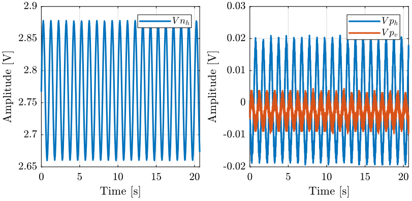

Identification signals when exciting the horizontal direction (png, pdf)

  <<plt-matlab>>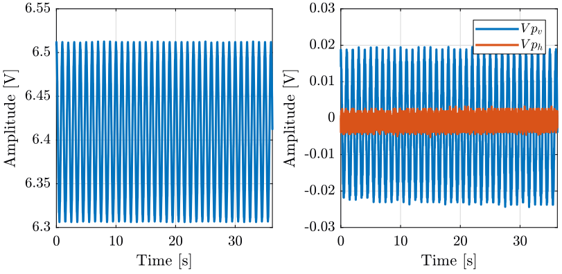

Identification signals when exciting in the vertical direction (png, pdf)

Linear Regression to obtain the gain of the 4QD

We plot the angle of mirror

Gain of the Newport metrology in [rad/V].

  gn0 = 2.62e-3;

The angular displacement of the beam is twice the angular displacement of the Newport mirror.

We do a linear regression \[ y = a x + b \] where:

• $y$ is the measured voltage of the 4QD in [V]
• $x$ is the beam angle (twice the mirror angle) in [rad]
• $a$ is the identified gain of the 4QD in [rad/V]

The linear regression is shown in Fig. fig:4qd_linear_reg.

  bh = [ones(size(uh.Vnh)) 2*gn0*uh.Vnh]\uh.Vph;
  bv = [ones(size(uv.Vnv)) 2*gn0*uv.Vnv]\uv.Vpv;

  <<plt-matlab>>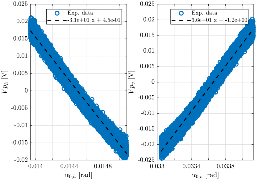

Linear Regression (png, pdf)

Thus, we obtain the "gain of the 4 quadrant photo-diode as shown on table tab:gain_4qd.

Horizontal [V/rad]	Vertical [V/rad]
-31.0	36.3

Identified Gain of the 4 quadrant diode

  Gd = tf([bh(2) 0 ;
           0     bv(2)]);

We obtain:

\begin{align*} \frac{V_{qd,h}}{\alpha_{0,h}} &\approx 0.032\ \left[ \frac{rad}{V} \right] \\ &\approx 32.3\ \left[ \frac{\mu rad}{mV} \right] \end{align*} \begin{align*} \frac{V_{qd,v}}{\alpha_{0,v}} &\approx 0.028\ \left[ \frac{rad}{V} \right] \\ &\approx 27.6\ \left[ \frac{\mu rad}{mV} \right] \end{align*}

Identification of the Cercalo Impedance, Current Amplifier and Voltage Amplifier dynamics

Introduction   ignore

We wish here to determine $G_i$ and $G_a$ shown in Fig. fig:block_diagram_simplify.

We ignore the electro-mechanical coupling.

Electrical Schematic

The schematic of the electrical circuit used to drive the Cercalo is shown in Fig. fig:current_amplifier.

Current Amplifier Schematic

The elements are:

• $U_c$: the voltage generated by the DAC
• BUF: is a unity-gain open-loop buffer that allows to increase the output current
• $R$: a chosen resistor that will determine the gain of the current amplifier
• $L_c$: inductor present in the Cercalo
• $R_c$: resistance of the inductor
• $\tilde{V}_c$: voltage measured across the Cercalo's inductor
• $V_c$: amplified voltage measured across the Cercalo's inductor
• $I_c$ is the current going through the Cercalo's inductor

The values of the components have been measured for the horizontal and vertical directions:

• $R_h = 41 \Omega$
• $L_{c,h} = 0.1 mH$
• $R_{c,h} = 9.3 \Omega$
• $R_v = 41 \Omega$
• $L_{c,v} = 0.1 mH$
• $R_{c,v} = 8.3 \Omega$

Let's first determine the transfer function from $U_c$ to $I_c$.

We have that: \[ U_c = (R + R_c) I_c + L_c s I_c \]

Thus:

\begin{align} G_i(s) &= \frac{I_c}{U_c} \\ &= \frac{1}{(R + R_c) + L_c s} \\ &= \frac{G_{i,0}}{1 + s/\omega_0} \end{align}

with

• $G_{i,0} = \frac{1}{R + R_c}$
• $\omega_0 = \frac{R + R_c}{L_c}$

Now, determine the transfer function from $I_c$ to $\tilde{V}_c$: \[ \tilde{V}_C = R_c I_c + L_c s I_c \] Thus:

\begin{align} Z_c(s) &= \frac{\tilde{V}_c}{I_c} \\ &= R_c + L_c s \end{align}

Finally, the transfer function of the voltage amplifier $G_a$ is simply a low pass filter:

\begin{align} G_a(s) &= \frac{V_c}{\tilde{V}_c} \\ &= \frac{G_{a,0}}{1 + s/\omega_c} \end{align}

with

• $G_{a,0}$ is the gain 1000 (60dB)
• $\omega_c$ is the cut-off frequency of the voltage amplifier set to 1000Hz

Theoretical Transfer Functions

The values of the components in the current amplifier have been measured.

  Rh = 41; % [Ohm]
  Lch = 0.1e-3; % [H]
  Rch = 9.3; % [Ohm]

  Rv = 41; % [Ohm]
  Lcv = 0.1e-3; % [H]
  Rcv = 8.3; % [Ohm]

\begin{align*} G_i(s) &= \frac{1}{(R + R_c) + L_c s} \\ Z_c(s) &= R_c + L_c s \\ G_a(s) &= \frac{1000}{1 + s/\omega_c} \end{align*}

  Gi = blkdiag(1/(Rh + Rch + Lch * s), 1/(Rv + Rcv + Lcv * s));
  Zc = blkdiag(Rch+Lch*s, Rcv+Lcv*s);
  Ga = blkdiag(1000/(1 + s/2/pi/1000), 1000/(1 + s/2/pi/1000));

  <<plt-matlab>>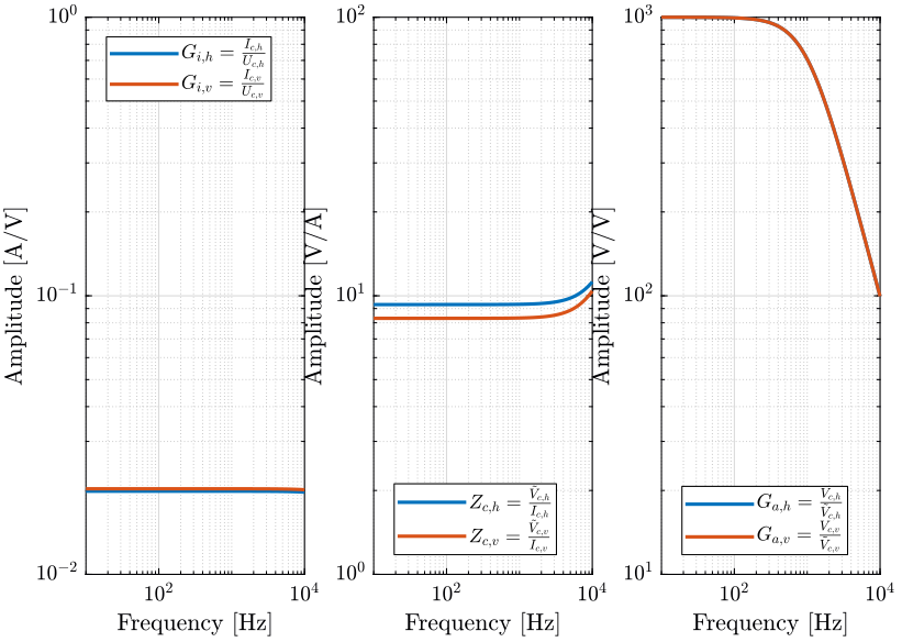

Transfer function for the current amplifier (png, pdf)

Over the frequency band of interest, the current amplifier transfer function $G_i$ can be considered as constant. This is the same for the impedance $Z_c$.

  Gi = tf(blkdiag(1/(Rh + Rch), 1/(Rv + Rcv)));
  Zc = tf(blkdiag(Rch, Rcv));

Identified Transfer Functions

Noise is generated using the DAC ($[U_{c,h}\ U_{c,v}]$) and we measure the output of the voltage amplifier $[V_{c,h}, V_{c,v}]$. From that, we should be able to identify $G_a Z_c G_i$.

The identification data is loaded.

  uh = load('mat/data_uch.mat', 't', 'Uch', 'Vch');
  uv = load('mat/data_ucv.mat', 't', 'Ucv', 'Vcv');

We remove the first seconds where the Cercalo is turned on.

  win = hanning(ceil(1*fs));
  [GaZcGi_h, f] = tfestimate(uh.Uch, uh.Vch, win, [], [], fs);
  [GaZcGi_v, ~] = tfestimate(uv.Ucv, uv.Vcv, win, [], [], fs);

  <<plt-matlab>>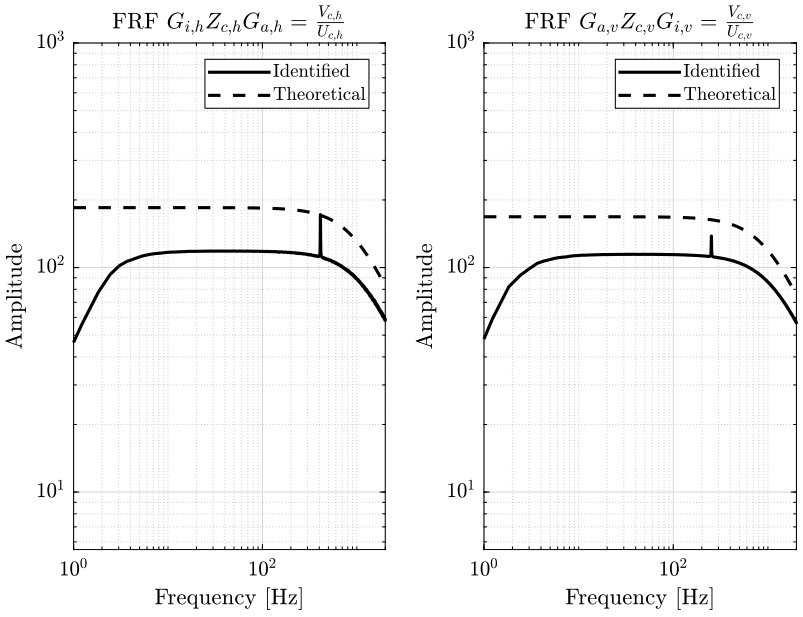

Identified and Theoretical Transfer Function $G_a G_i$ (png, pdf)

There is a gain mismatch, that is probably due to bad identification of the inductance and resistance measurement of the cercalo inductors. Thus, we suppose $G_a$ is perfectly known (the gain and cut-off frequency of the voltage amplifier is very accurate) and that $G_i$ is also well determined as it mainly depends on the resistor used in the amplifier that is well measured.

  Gi_resp_h = abs(GaZcGi_h)./squeeze(abs(freqresp(Ga(1,1)*Zc(1,1), f, 'Hz')));
  Gi_resp_v = abs(GaZcGi_v)./squeeze(abs(freqresp(Ga(2,2)*Zc(2,2), f, 'Hz')));
  Gi = tf(blkdiag(mean(Gi_resp_h(f>20 & f<200)), mean(Gi_resp_v(f>20 & f<200))));

  <<plt-matlab>>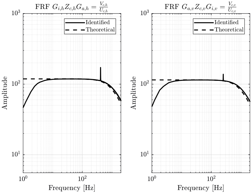

Identified and Theoretical Transfer Function $G_a G_i$ (png, pdf)

Finally, we have the following transfer functions:

ans = filepath;
if ischar(ans), fid = fopen('/tmp/babel-ZKMGJu/matlab-FA7h5L', 'w'); fprintf(fid, '%s\n', ans); fclose(fid);
else, dlmwrite('/tmp/babel-ZKMGJu/matlab-FA7h5L', ans, '\t')
end
'org_babel_eoe'
Gi,Zc,Ga
'org_babel_eoe'
ans = filepath;
if ischar(ans), fid = fopen('/tmp/babel-ZKMGJu/matlab-FA7h5L', 'w'); fprintf(fid, '%s\n', ans); fclose(fid);
else, dlmwrite('/tmp/babel-ZKMGJu/matlab-FA7h5L', ans, '\t')
end
'org_babel_eoe'
ans =
    'org_babel_eoe'
Gi,Zc,Ga

Gi =

  From input 1 to output...
   1:  0.01275

   2:  0

  From input 2 to output...
   1:  0

   2:  0.01382

Static gain.


Zc =

  From input 1 to output...
   1:  9.3

   2:  0

  From input 2 to output...
   1:  0

   2:  8.3

Static gain.


Ga =

  From input 1 to output...
       6.2832e+06
   1:  ----------
        (s+6283)

   2:  0

  From input 2 to output...
   1:  0

       6.2832e+06
   2:  ----------
        (s+6283)

Continuous-time zero/pole/gain model.

Identification of the Cercalo Dynamics

Introduction   ignore

We now wish to identify the dynamics of the Cercalo identified by $G_c$ on the block diagram in Fig. fig:block_diagram_simplify.

To do so, we inject some noise at the input of the current amplifier $[U_{c,h},\ U_{c,v}]$ (one input after the other) and we measure simultaneously the output of the 4QD $[V_{p,h},\ V_{p,v}]$.

The transfer function obtained will be $G_c G_i$, and because we have already identified $G_i$, we can obtain $G_c$ by multiplying the obtained transfer function matrix by ${G_i}^{-1}$.

Input / Output data

The identification data is loaded

  uh = load('mat/data_uch.mat', 't', 'Uch', 'Vph', 'Vpv');
  uv = load('mat/data_ucv.mat', 't', 'Ucv', 'Vph', 'Vpv');

We remove the first seconds where the Cercalo is turned on.

  t0 = 1;

  uh.Uch(uh.t<t0) = [];
  uh.Vph(uh.t<t0) = [];
  uh.Vpv(uh.t<t0) = [];
  uh.t(uh.t<t0)   = [];
  uh.t = uh.t - uh.t(1); % We start at t=0

  t0 = 1;

  uv.Ucv(uv.t<t0) = [];
  uv.Vph(uv.t<t0) = [];
  uv.Vpv(uv.t<t0) = [];
  uv.t(uv.t<t0)   = [];

  uv.t = uv.t - uv.t(1); % We start at t=0

  <<plt-matlab>>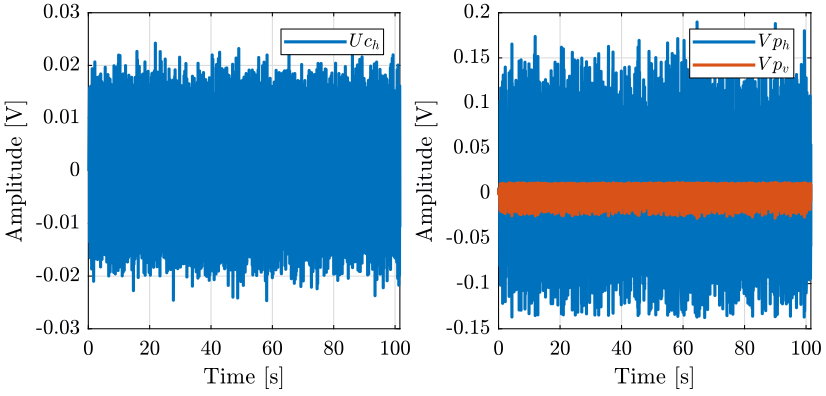

Identification signals when exciting the horizontal direction (png, pdf)

  <<plt-matlab>>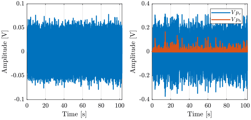

Identification signals when exciting in the vertical direction (png, pdf)

Coherence

The window used for the spectral analysis is an hanning windows with temporal size equal to 1 second.

  win = hanning(ceil(1*fs));

  [coh_Uch_Vph, f] = mscohere(uh.Uch, uh.Vph, win, [], [], fs);
  [coh_Uch_Vpv, ~] = mscohere(uh.Uch, uh.Vpv, win, [], [], fs);
  [coh_Ucv_Vph, ~] = mscohere(uv.Ucv, uv.Vph, win, [], [], fs);
  [coh_Ucv_Vpv, ~] = mscohere(uv.Ucv, uv.Vpv, win, [], [], fs);

  <<plt-matlab>>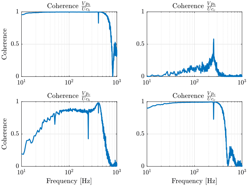

Coherence (png, pdf)

Estimation of the Frequency Response Function Matrix

We compute an estimate of the transfer functions.

  [tf_Uch_Vph, f] = tfestimate(uh.Uch, uh.Vph, win, [], [], fs);
  [tf_Uch_Vpv, ~] = tfestimate(uh.Uch, uh.Vpv, win, [], [], fs);
  [tf_Ucv_Vph, ~] = tfestimate(uv.Ucv, uv.Vph, win, [], [], fs);
  [tf_Ucv_Vpv, ~] = tfestimate(uv.Ucv, uv.Vpv, win, [], [], fs);

  <<plt-matlab>>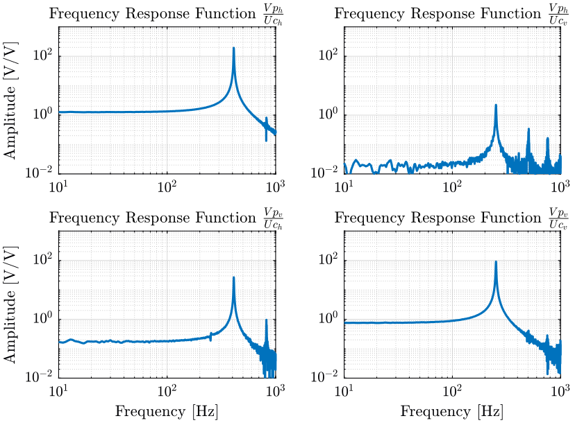

Frequency Response Matrix (png, pdf)

  <<plt-matlab>>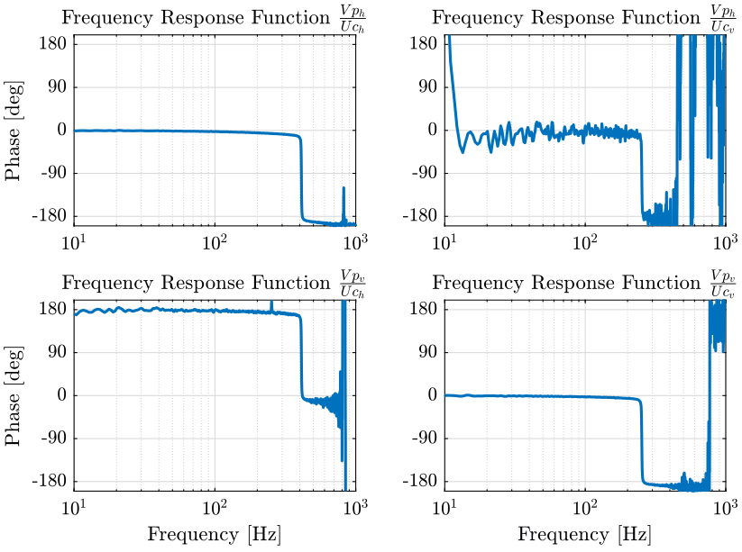

Frequency Response Matrix_Phase (png, pdf)

Time Delay

Now, we would like to remove the time delay included in the FRF prior to the model extraction.

Estimation of the time delay:

  Ts_delay = Ts; % [s]

  G_delay = tf(1, 1, 'InputDelay', Ts_delay);

  G_delay_resp = squeeze(freqresp(G_delay, f, 'Hz'));

We then remove the time delay from the frequency response function.

  tf_Uch_Vph = tf_Uch_Vph./G_delay_resp;
  tf_Uch_Vpv = tf_Uch_Vpv./G_delay_resp;
  tf_Ucv_Vph = tf_Ucv_Vph./G_delay_resp;
  tf_Ucv_Vpv = tf_Ucv_Vpv./G_delay_resp;

Extraction of a transfer function matrix

First we define the initial guess for the resonance frequencies and the weights associated.

  freqs_res_uh = [410]; % [Hz]
  freqs_res_uv = [250]; % [Hz]

We then make an initial guess on the complex values of the poles.

  xi = 0.001; % Approximate modal damping
  poles_uh = [2*pi*freqs_res_uh*(xi + 1i), 2*pi*freqs_res_uh*(xi - 1i)];
  poles_uv = [2*pi*freqs_res_uv*(xi + 1i), 2*pi*freqs_res_uv*(xi - 1i)];

We then define the weight that will be used for the fitting. Basically, we want more weight around the resonance and at low frequency (below the first resonance). Also, we want more importance where we have a better coherence. Finally, we ignore data above some frequency.

  weight_Uch_Vph = coh_Uch_Vph';
  weight_Uch_Vpv = coh_Uch_Vpv';
  weight_Ucv_Vph = coh_Ucv_Vph';
  weight_Ucv_Vpv = coh_Ucv_Vpv';

  alpha = 0.1;

  for freq_i = 1:length(freqs_res_uh)
    weight_Uch_Vph(f>(1-alpha)*freqs_res_uh(freq_i) & f<(1 + alpha)*freqs_res_uh(freq_i)) = 10;
    weight_Uch_Vpv(f>(1-alpha)*freqs_res_uh(freq_i) & f<(1 + alpha)*freqs_res_uh(freq_i)) = 10;
    weight_Ucv_Vph(f>(1-alpha)*freqs_res_uv(freq_i) & f<(1 + alpha)*freqs_res_uv(freq_i)) = 10;
    weight_Ucv_Vpv(f>(1-alpha)*freqs_res_uv(freq_i) & f<(1 + alpha)*freqs_res_uv(freq_i)) = 10;
  end

  weight_Uch_Vph(f>1000) = 0;
  weight_Uch_Vpv(f>1000) = 0;
  weight_Ucv_Vph(f>1000) = 0;
  weight_Ucv_Vpv(f>1000) = 0;

The weights are shown in Fig. fig:weights_cercalo.

  <<plt-matlab>>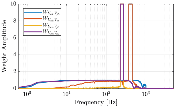

Weights amplitude (png, pdf)

When we set some options for vfit3.

  opts = struct();

  opts.stable = 1;    % Enforce stable poles
  opts.asymp = 1;     % Force D matrix to be null
  opts.relax = 1;     % Use vector fitting with relaxed non-triviality constraint
  opts.skip_pole = 0; % Do NOT skip pole identification
  opts.skip_res = 0;  % Do NOT skip identification of residues (C,D,E)
  opts.cmplx_ss = 0;  % Create real state space model with block diagonal A

  opts.spy1 = 0;      % No plotting for first stage of vector fitting
  opts.spy2 = 0;      % Create magnitude plot for fitting of f(s)

We define the number of iteration.

  Niter = 5;

An we run the vectfit3 algorithm.

  for iter = 1:Niter
    [SER_Uch_Vph, poles, ~, fit_Uch_Vph] = vectfit3(tf_Uch_Vph.', 1i*2*pi*f, poles_uh, weight_Uch_Vph, opts);
  end
  for iter = 1:Niter
    [SER_Uch_Vpv, poles, ~, fit_Uch_Vpv] = vectfit3(tf_Uch_Vpv.', 1i*2*pi*f, poles_uh, weight_Uch_Vpv, opts);
  end
  for iter = 1:Niter
    [SER_Ucv_Vph, poles, ~, fit_Ucv_Vph] = vectfit3(tf_Ucv_Vph.', 1i*2*pi*f, poles_uv, weight_Ucv_Vph, opts);
  end
  for iter = 1:Niter
    [SER_Ucv_Vpv, poles, ~, fit_Ucv_Vpv] = vectfit3(tf_Ucv_Vpv.', 1i*2*pi*f, poles_uv, weight_Ucv_Vpv, opts);
  end

  <<plt-matlab>>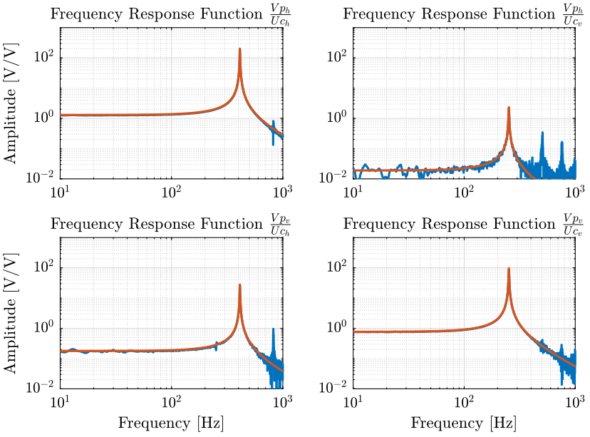

Transfer Function Extraction of the FRF matrix (png, pdf)

  <<plt-matlab>>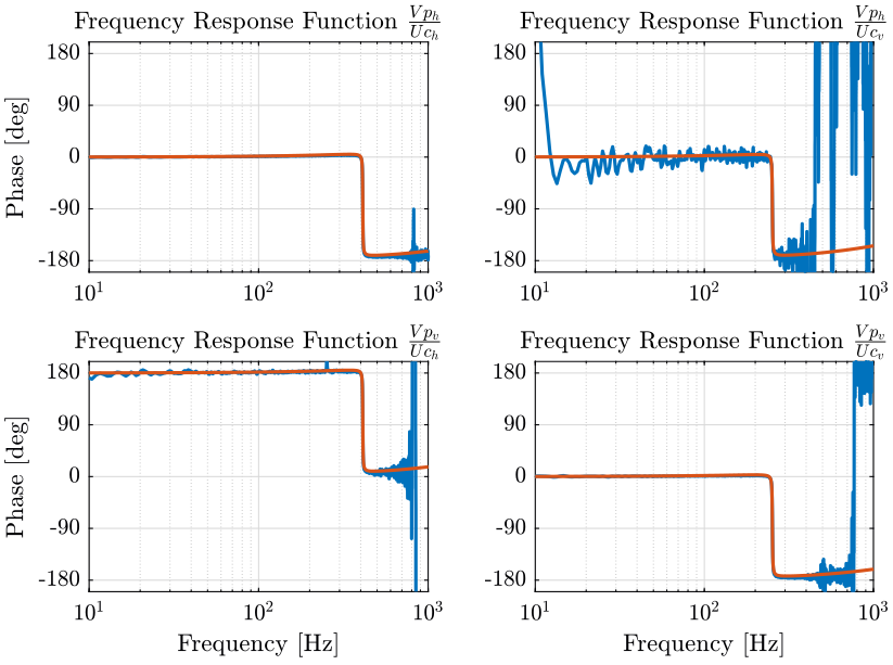

Transfer Function Extraction of the FRF matrix (png, pdf)

And finally, we create the identified $G_c$ matrix by multiplying by ${G_i}^{-1}$.

  G_Uch_Vph = tf(minreal(ss(full(SER_Uch_Vph.A),SER_Uch_Vph.B,SER_Uch_Vph.C,SER_Uch_Vph.D)));
  G_Ucv_Vph = tf(minreal(ss(full(SER_Ucv_Vph.A),SER_Ucv_Vph.B,SER_Ucv_Vph.C,SER_Ucv_Vph.D)));
  G_Uch_Vpv = tf(minreal(ss(full(SER_Uch_Vpv.A),SER_Uch_Vpv.B,SER_Uch_Vpv.C,SER_Uch_Vpv.D)));
  G_Ucv_Vpv = tf(minreal(ss(full(SER_Ucv_Vpv.A),SER_Ucv_Vpv.B,SER_Ucv_Vpv.C,SER_Ucv_Vpv.D)));

  Gc = [G_Uch_Vph, G_Ucv_Vph;
        G_Uch_Vpv, G_Ucv_Vpv]*inv(Gi);

Identification of the Newport Dynamics

Introduction   ignore

We here identify the transfer function from a reference sent to the Newport $[U_{n,h},\ U_{n,v}]$ to the measurement made by the 4QD $[V_{p,h},\ V_{p,v}]$.

To do so, we inject noise to the Newport $[U_{n,h},\ U_{n,v}]$ and we record the 4QD measurement $[V_{p,h},\ V_{p,v}]$.

Input / Output data

The identification data is loaded

  uh = load('mat/data_unh.mat', 't', 'Unh', 'Vph', 'Vpv');
  uv = load('mat/data_unv.mat', 't', 'Unv', 'Vph', 'Vpv');

We remove the first seconds where the Cercalo is turned on.

  t0 = 3;

  uh.Unh(uh.t<t0) = [];
  uh.Vph(uh.t<t0) = [];
  uh.Vpv(uh.t<t0) = [];
  uh.t(uh.t<t0)   = [];
  uh.t = uh.t - uh.t(1); % We start at t=0

  t0 = 1.5;

  uv.Unv(uv.t<t0) = [];
  uv.Vph(uv.t<t0) = [];
  uv.Vpv(uv.t<t0) = [];
  uv.t(uv.t<t0)   = [];

  uv.t = uv.t - uv.t(1); % We start at t=0

  <<plt-matlab>>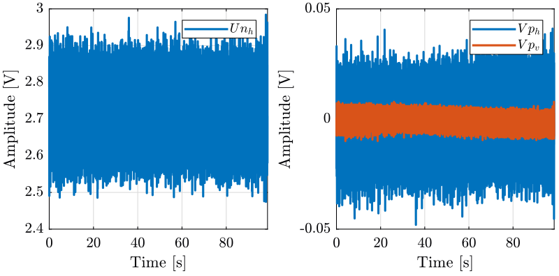

Identification signals when exciting the horizontal direction (png, pdf)

  <<plt-matlab>>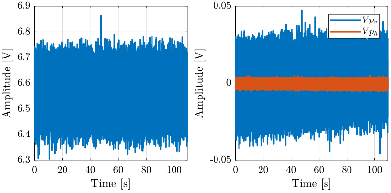

Identification signals when exciting in the vertical direction (png, pdf)

Coherence

The window used for the spectral analysis is an hanning windows with temporal size equal to 1 second.

  win = hanning(ceil(1*fs));

  [coh_Unh_Vph, f] = mscohere(uh.Unh, uh.Vph, win, [], [], fs);
  [coh_Unh_Vpv, ~] = mscohere(uh.Unh, uh.Vpv, win, [], [], fs);
  [coh_Unv_Vph, ~] = mscohere(uv.Unv, uv.Vph, win, [], [], fs);
  [coh_Unv_Vpv, ~] = mscohere(uv.Unv, uv.Vpv, win, [], [], fs);

  <<plt-matlab>>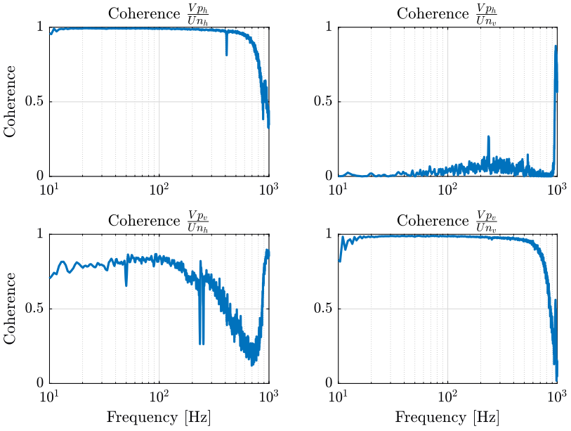

Coherence (png, pdf)

Estimation of the Frequency Response Function Matrix

We compute an estimate of the transfer functions.

  [tf_Unh_Vph, f] = tfestimate(uh.Unh, uh.Vph, win, [], [], fs);
  [tf_Unh_Vpv, ~] = tfestimate(uh.Unh, uh.Vpv, win, [], [], fs);
  [tf_Unv_Vph, ~] = tfestimate(uv.Unv, uv.Vph, win, [], [], fs);
  [tf_Unv_Vpv, ~] = tfestimate(uv.Unv, uv.Vpv, win, [], [], fs);

  <<plt-matlab>>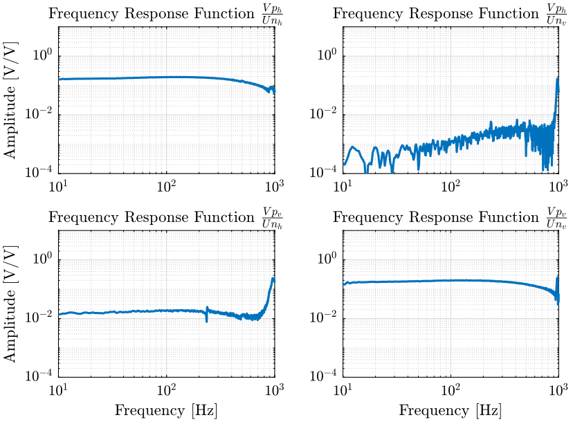

Frequency Response Matrix (png, pdf)

  <<plt-matlab>>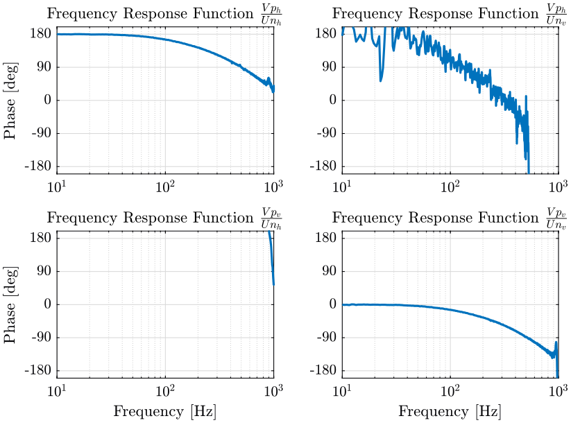

Frequency Response Matrix Phase (png, pdf)

Time Delay

Now, we would like to remove the time delay included in the FRF prior to the model extraction.

Estimation of the time delay:

  Ts_delay = 0.0005; % [s]

  G_delay = tf(1, 1, 'InputDelay', Ts_delay);

  G_delay_resp = squeeze(freqresp(G_delay, f, 'Hz'));

We then remove the time delay from the frequency response function.

  <<plt-matlab>>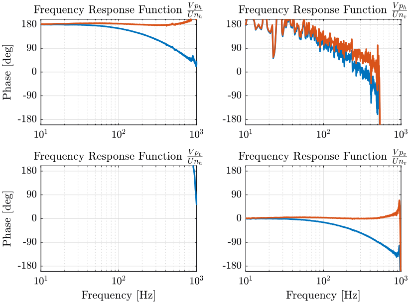

Phase change due to time-delay in the Newport dynamics (png, pdf)

Extraction of a transfer function matrix

From Fig. fig:frf_newport_gain, it seems reasonable to model the Newport dynamics as diagonal and constant.

  Gn = blkdiag(tf(mean(abs(tf_Unh_Vph(f>10 & f<100)))), tf(mean(abs(tf_Unv_Vpv(f>10 & f<100)))));

Full System

We now have identified:

• $G_i$
• $G_a$
• $G_c$
• $G_n$
• $G_d$

We name the input and output of each transfer function:

  Gi.InputName = {'Uch', 'Ucv'};
  Gi.OutputName = {'Ich', 'Icv'};

  Zc.InputName = {'Ich', 'Icv'};
  Zc.OutputName = {'Vtch', 'Vtcv'};

  Ga.InputName = {'Vtch', 'Vtcv'};
  Ga.OutputName = {'Vch', 'Vcv'};

  Gc.InputName = {'Ich', 'Icv'};
  Gc.OutputName = {'Vpch', 'Vpcv'};

  Gn.InputName = {'Unh', 'Unv'};
  Gn.OutputName = {'Vpnh', 'Vpnv'};

  Gd.InputName = {'Rh', 'Rv'};
  Gd.OutputName = {'Vph', 'Vpv'};

  Sh = sumblk('Vph = Vpch + Vpnh');
  Sv = sumblk('Vpv = Vpcv + Vpnv');

  inputs  = {'Uch', 'Ucv', 'Unh', 'Unv'};
  outputs = {'Vch', 'Vcv', 'Ich', 'Icv', 'Rh', 'Rv', 'Vph', 'Vpv'};

  sys = connect(Gi, Zc, Ga, Gc, Gn, inv(Gd), Sh, Sv, inputs, outputs);

The file mat/plant.mat is accessible here.

  save('mat/plant.mat', 'sys', 'Gi', 'Zc', 'Ga', 'Gc', 'Gn', 'Gd');

Active Damping

Load Plant

  load('mat/plant.mat', 'sys', 'Gi', 'Zc', 'Ga', 'Gc', 'Gn', 'Gd');

Test

  bode(sys({'Vch', 'Vcv'}, {'Uch', 'Ucv'}));

  Kppf = blkdiag(-10000/s, tf(0));

  Kppf.InputName  = {'Vch', 'Vcv'};
  Kppf.OutputName = {'Uch', 'Ucv'};

  inputs  = {'Uch', 'Ucv', 'Unh', 'Unv'};
  outputs = {'Ich', 'Icv', 'Rh', 'Rv', 'Vph', 'Vpv'};

  sys_cl = connect(sys, Kppf, inputs, outputs);

  figure; bode(sys_cl({'Vph', 'Vpv'}, {'Uch', 'Ucv'}), sys({'Vph', 'Vpv'}, {'Uch', 'Ucv'}))

TODO Huddle Test

We load the data taken during the Huddle Test.

  load('mat/data_huddle_test.mat', ...
       't', 'Uch', 'Ucv', ...
       'Unh', 'Unv', ...
       'Vph', 'Vpv', ...
       'Vch', 'Vcv', ...
       'Vnh', 'Vnv', ...
       'Va');

We remove the first second of data where everything is settling down.

  t0 = 1;

  Uch(t<t0) = [];
  Ucv(t<t0) = [];
  Unh(t<t0) = [];
  Unv(t<t0) = [];
  Vph(t<t0) = [];
  Vpv(t<t0) = [];
  Vch(t<t0) = [];
  Vcv(t<t0) = [];
  Vnh(t<t0) = [];
  Vnv(t<t0) = [];
  Va(t<t0)  = [];
  t(t<t0)   = [];

  t = t - t(1); % We start at t=0

We compute the Power Spectral Density of the horizontal and vertical positions of the beam as measured by the 4 quadrant diode.

  [psd_Vph, f] = pwelch(Vph, hanning(ceil(1*fs)), [], [], fs);
  [psd_Vpv, ~] = pwelch(Vpv, hanning(ceil(1*fs)), [], [], fs);

  figure;
  hold on;
  plot(f, sqrt(psd_Vph), 'DisplayName', '$\Gamma_{Vp_h}$');
  plot(f, sqrt(psd_Vpv), 'DisplayName', '$\Gamma_{Vp_v}$');
  hold off;
  set(gca, 'xscale', 'log'); set(gca, 'yscale', 'log');
  xlabel('Frequency [Hz]'); ylabel('ASD $\left[\frac{V}{\sqrt{Hz}}\right]$')
  legend('Location', 'southwest');
  xlim([1, 1000]);

We compute the Power Spectral Density of the voltage across the inductance used for horizontal and vertical positioning of the Cercalo.

  [psd_Vch, f] = pwelch(Vch, hanning(ceil(1*fs)), [], [], fs);
  [psd_Vcv, ~] = pwelch(Vcv, hanning(ceil(1*fs)), [], [], fs);

  figure;
  hold on;
  plot(f, sqrt(psd_Vch), 'DisplayName', '$\Gamma_{Vc_h}$');
  plot(f, sqrt(psd_Vcv), 'DisplayName', '$\Gamma_{Vc_v}$');
  hold off;
  set(gca, 'xscale', 'log'); set(gca, 'yscale', 'log');
  xlabel('Frequency [Hz]'); ylabel('ASD $\left[\frac{V}{\sqrt{Hz}}\right]$')
  legend('Location', 'southwest');
  xlim([1, 1000]);

Plant Scaling

	Value	Unit
Expected perturbations	1	[V]	$U_n$
Maximum input usage	10	[V]	$U_c$
Maximum wanted error	10	[$\mu rad$]	$\theta$
Measured noise	5	[$\mu rad$]

General Configuration

Plant Analysis

Load Plant

  load('mat/plant.mat', 'G');

RGA-Number

  freqs = logspace(2, 4, 1000);
  G_resp = freqresp(G, freqs, 'Hz');
  A = zeros(size(G_resp));
  RGAnum = zeros(1, length(freqs));

  for i = 1:length(freqs)
    A(:, :, i) = G_resp(:, :, i).*inv(G_resp(:, :, i))';
    RGAnum(i) = sum(sum(abs(A(:, :, i)-eye(2))));
  end
  % RGA = G0.*inv(G0)';

  figure;
  plot(freqs, RGAnum);
  set(gca, 'xscale', 'log');

  U = zeros(2, 2, length(freqs));
  S = zeros(2, 2, length(freqs))
  V = zeros(2, 2, length(freqs));

  for i = 1:length(freqs)
    [Ui, Si, Vi] = svd(G_resp(:, :, i));
    U(:, :, i) = Ui;
    S(:, :, i) = Si;
    V(:, :, i) = Vi;
  end

Rotation Matrix

  G0 = freqresp(G, 0);

Control Objective

The maximum expected stroke is $y_\text{max} = 3mm \approx 5e^{-2} rad$ at $1Hz$. The maximum wanted error is $e_\text{max} = 10 \mu rad$.

Thus, we require the sensitivity function at $\omega_0 = 1\text{ Hz}$:

\begin{align*} |S(j\omega_0)| &< \left| \frac{e_\text{max}}{y_\text{max}} \right| \\ &< 2 \cdot 10^{-4} \end{align*}

In terms of loop gain, this is equivalent to: \[ |L(j\omega_0)| > 5 \cdot 10^{3} \]

Decentralized Control

<<sec:decentralized_control>>

Introduction   ignore

In this section, we try to implement a simple decentralized controller.

ZIP file containing the data and matlab files   ignore

All the files (data and Matlab scripts) are accessible here.

Load Plant

  load('mat/plant.mat', 'sys', 'Gi', 'Zc', 'Ga', 'Gc', 'Gn', 'Gd');

Diagonal Controller

Using SISOTOOL, a diagonal controller is designed. The two SISO loop gains are shown in Fig. fig:diag_contr_loop_gain.

  Kh = -0.25598*(s+112)*(s^2 + 15.93*s + 6.686e06)/((s^2*(s+352.5)*(1+s/2/pi/2000)));
  Kv = 10207*(s+55.15)*(s^2 + 17.45*s + 2.491e06)/(s^2*(s+491.2)*(s+7695));

  K = blkdiag(Kh, Kv);
  K.InputName  = {'Rh', 'Rv'};
  K.OutputName = {'Uch', 'Ucv'};

  <<plt-matlab>>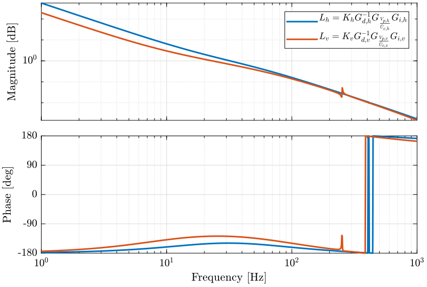

Loop Gain using the Decentralized Diagonal Controller (png, pdf)

We then close the loop and we look at the transfer function from the Newport rotation signal to the beam angle (Fig. fig:diag_contr_effect_newport).

  inputs  = {'Uch', 'Ucv', 'Unh', 'Unv'};
  outputs = {'Vch', 'Vcv', 'Ich', 'Icv', 'Rh', 'Rv', 'Vph', 'Vpv'};

  sys_cl = connect(sys, -K, inputs, outputs);

  <<plt-matlab>>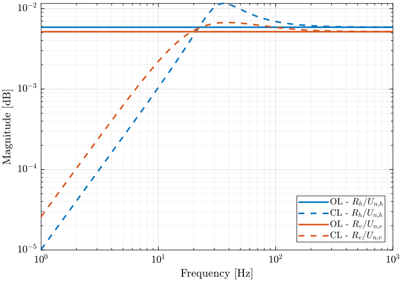

Effect of the Newport rotation on the beam position when the loop is closed using the Decentralized Diagonal Controller (png, pdf)

Save the Controller

  Kd = c2d(K, 1e-4, 'tustin');

The diagonal controller is accessible here.

  save('mat/K_diag.mat', 'K', 'Kd');

Newport Control

Introduction   ignore

In this section, we try to implement a simple decentralized controller for the Newport. This can be used to align the 4QD:

• once there is a signal from the 4QD, the Newport feedback loop is closed
• thus, the Newport is positioned such that the beam hits the center of the 4QD
• then we can move the 4QD manually in X-Y plane in order to cancel the command signal of the Newport
• finally, we are sure to be aligned when the command signal of the Newport is 0

Load Plant

  load('mat/plant.mat', 'Gn', 'Gd');

Analysis

The plant is basically a constant until frequencies up to the required bandwidth.

We get that constant value.

  Gn0 = freqresp(inv(Gd)*Gn, 0);

We design two controller containing 2 integrators and one lead near the crossover frequency set to 10Hz.

  h = 2;
  w0 = 2*pi*10;

  Knh = 1/Gn0(1,1) * (w0/s)^2 * (1 + s/w0*h)/(1 + s/w0/h)/h;
  Knv = 1/Gn0(2,2) * (w0/s)^2 * (1 + s/w0*h)/(1 + s/w0/h)/h;

  <<plt-matlab>>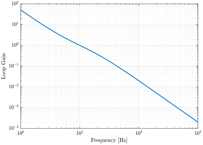

Diagonal Loop Gain for the Newport (png, pdf)

Save

  Kn = blkdiag(Knh, Knv);
  Knd = c2d(Kn, 1e-4, 'tustin');

The controllers can be downloaded here.

  save('mat/K_newport.mat', 'Kn', 'Knd');

Measurement of the non-repeatability

Data Load

  load('mat/data_rep_1.mat', ...
       't', 'Uch', 'Ucv', ...
       'Unh', 'Unv', ...
       'Vph', 'Vpv', ...
       'Vch', 'Vcv', ...
       'Vnh', 'Vnv', ...
       'Va');

  t0 = 5;

  Uch(t<t0) = [];
  Ucv(t<t0) = [];
  Unh(t<t0) = [];
  Unv(t<t0) = [];
  Vph(t<t0) = [];
  Vpv(t<t0) = [];
  Vch(t<t0) = [];
  Vcv(t<t0) = [];
  Vnh(t<t0) = [];
  Vnv(t<t0) = [];
  Va(t<t0)  = [];
  t(t<t0)   = [];

  t = t - t(1); % We start at t=0

TODO Some Plots

Repeatability

  bh = [ones(size(Vnh)) Vnh]\Vph;
  bv = [ones(size(Vnv)) Vnv]\Vpv;