75 KiB
NASS - Finite Element Models with Simscape
- Introduction
- APA300ML
- Introduction
- Import Mass Matrix, Stiffness Matrix, and Interface Nodes Coordinates
- Piezoelectric parameters
- Simscape Model
- Identification of the APA Characteristics
- Identification of the Dynamics from actuator to replace displacement
- Identification of the Dynamics from actuator to force sensor
- Identification for a simpler model
- Integral Force Feedback
- First Flexible Joint Geometry
- Optimized Flexible Joint
- Complete Strut with Encoder
- Bibliography
This report is also available as a pdf.
Introduction ignore
In this document, Finite Element Models (FEM) of parts of the Nano-Hexapod are developed and integrated into Simscape for dynamical analysis.
It is divided in the following sections:
- Section sec:APA300ML: A super-element of the Amplified Piezoelectric Actuator APA300ML used for the NASS is exported using Ansys and imported in Simscape. The static and dynamical properties of the APA300ML are then estimated using the Simscape model.
- Section sec:flexor_ID16: A first geometry of a Flexible joint is modelled and its characteristics are identified from the Stiffness matrix as well as from the Simscape model.
- Section sec:flexor_025: An optimized flexible joint is developed for the Nano-Hexapod and is then imported in a Simscape model.
- Section sec:strut_encoder: A super element of a complete strut is studied.
APA300ML
<<sec:APA300ML>>
Introduction ignore
In this section, the Amplified Piezoelectric Actuator APA300ML (doc) is modeled using a Finite Element Software. Then a super element is exported and imported in Simscape where its dynamic is studied.
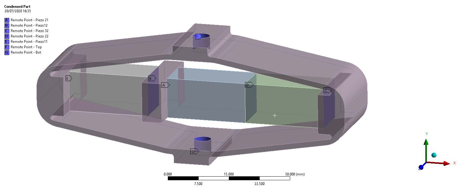
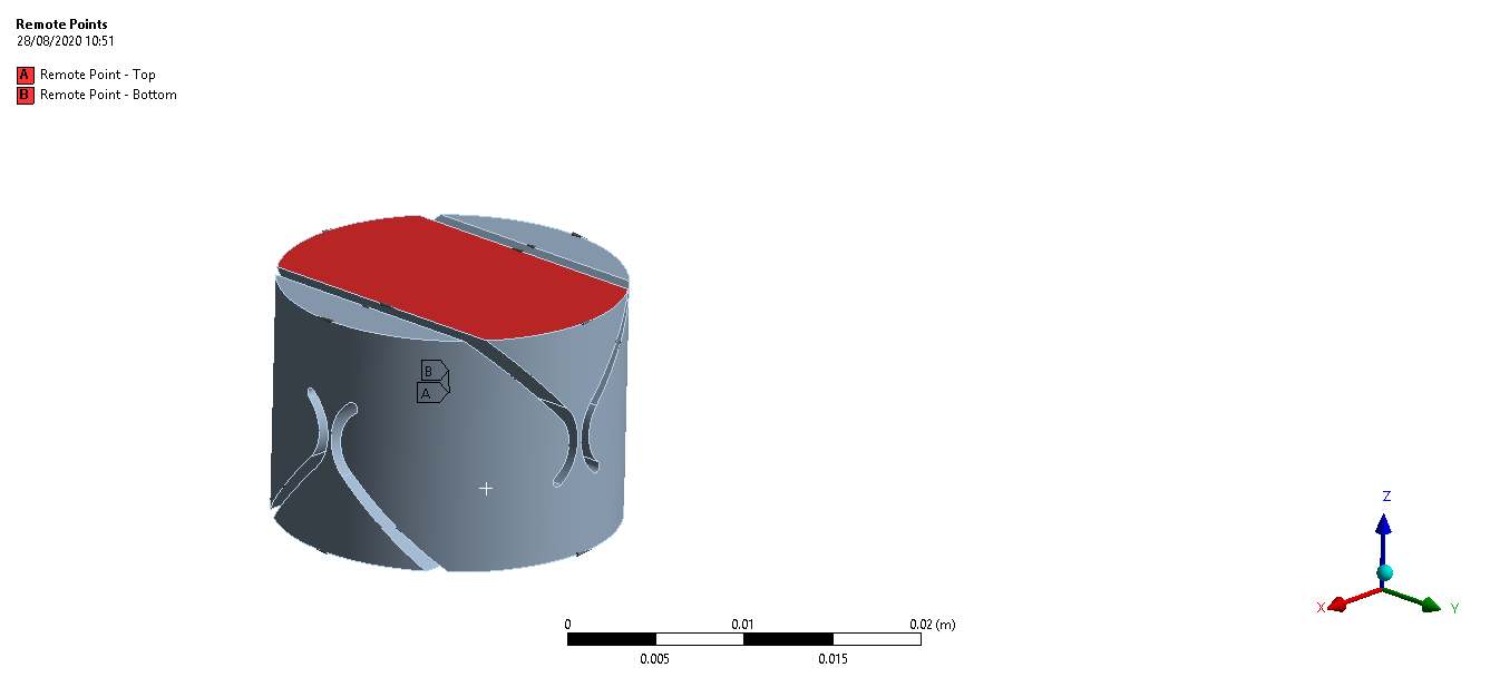
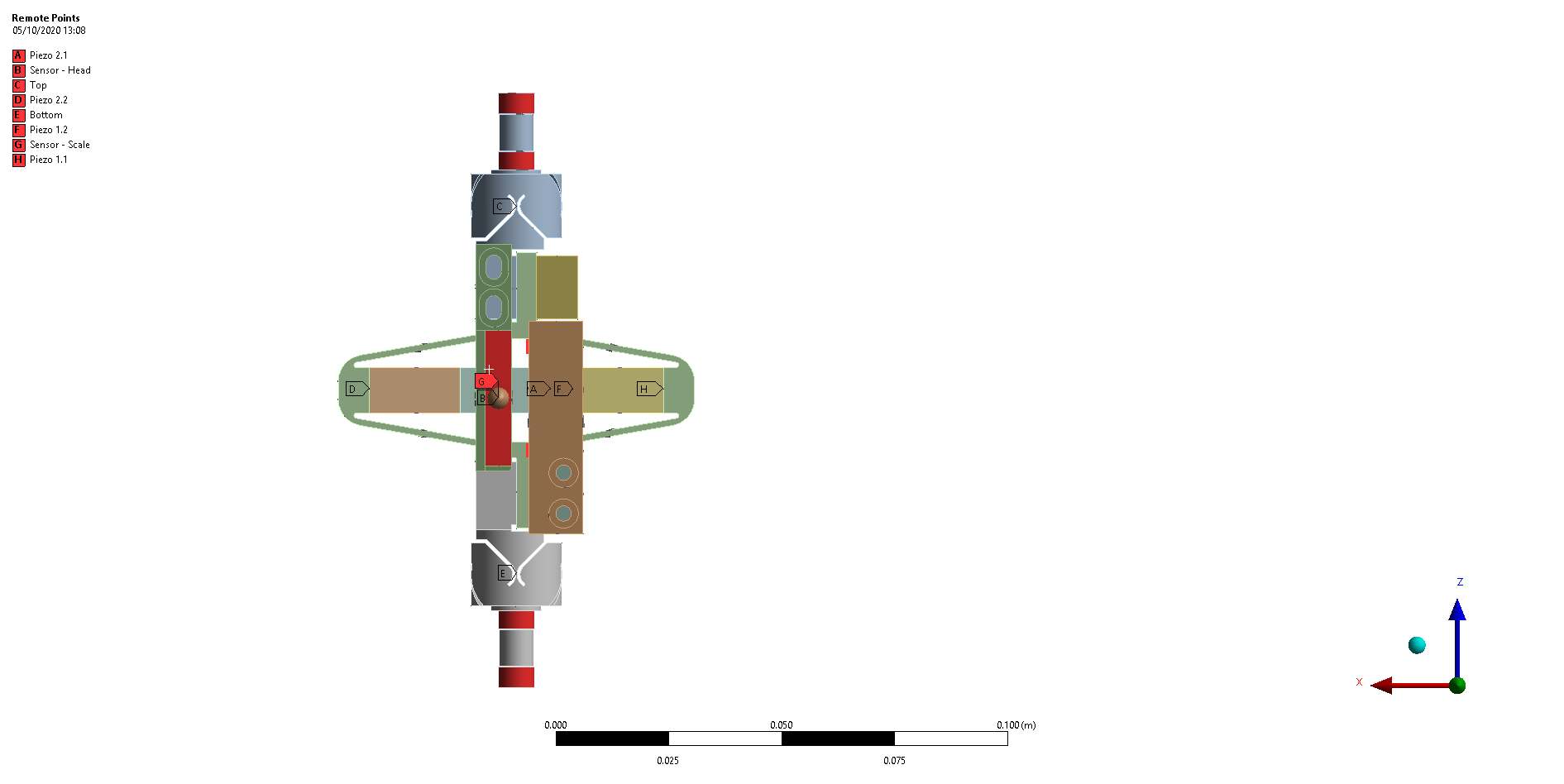
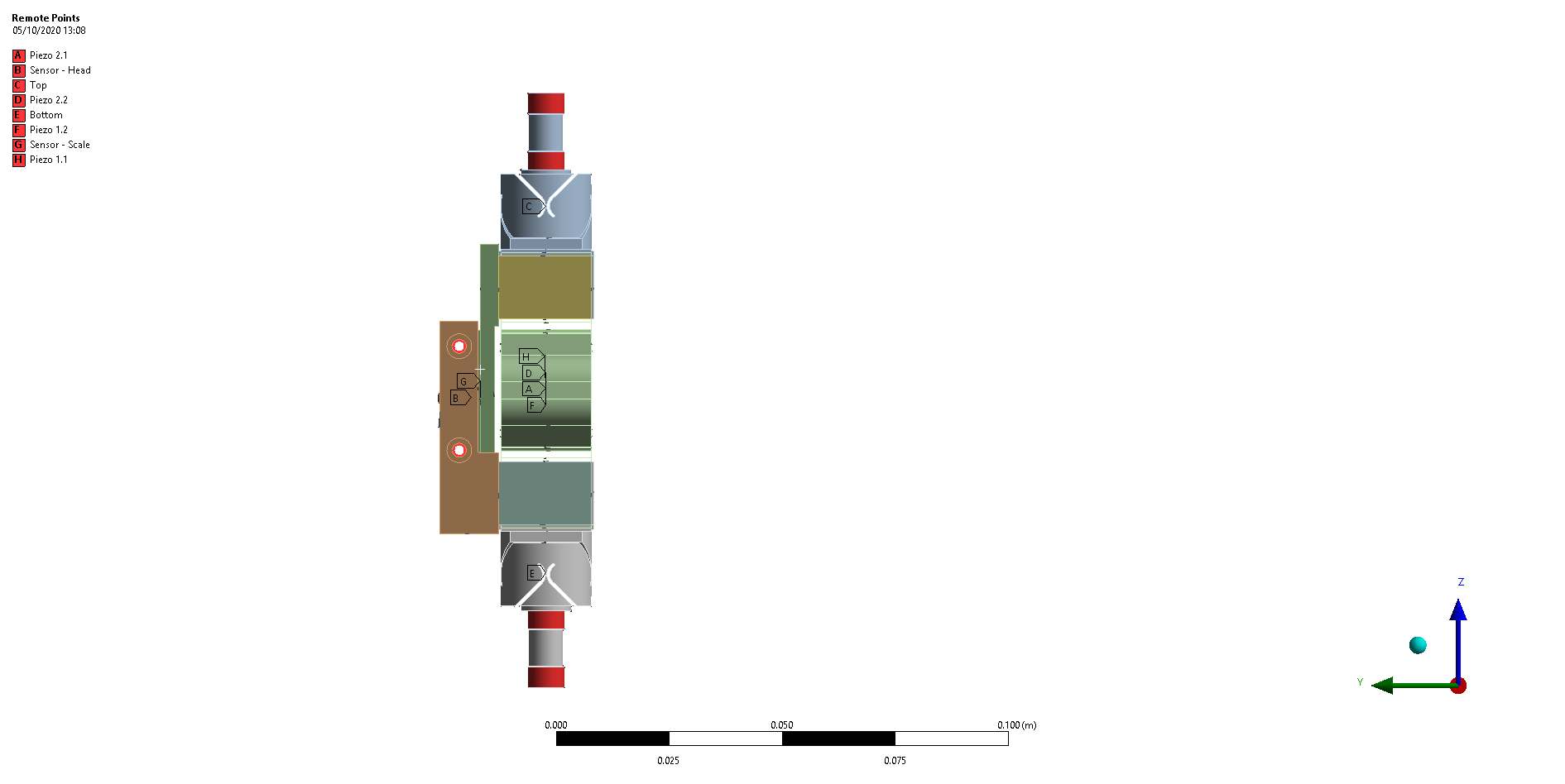
A 3D view of the Amplified Piezoelectric Actuator (APA300ML) is shown in Figure fig:apa300ml_ansys. The remote point used are also shown in this figure.
Import Mass Matrix, Stiffness Matrix, and Interface Nodes Coordinates
We first extract the stiffness and mass matrices.
K = readmatrix('APA300ML_mat_K.CSV');
M = readmatrix('APA300ML_mat_M.CSV');| 200000000 | 30000 | -20000 | -70 | 300000 | 40 | 10000000 | 10000 | -6000 | 30 |
| 30000 | 30000000 | 2000 | -200000 | 60 | -10 | 4000 | 2000000 | -500 | 9000 |
| -20000 | 2000 | 7000000 | -10 | -30 | 10 | 6000 | 900 | -500000 | 3 |
| -70 | -200000 | -10 | 1000 | -0.1 | 08 | -20 | -9000 | 3 | -30 |
| 300000 | 60 | -30 | -0.1 | 900 | 0.1 | 30000 | 20 | -10 | 06 |
| 40 | -10 | 10 | 08 | 0.1 | 10000 | 20 | 9 | -5 | 03 |
| 10000000 | 4000 | 6000 | -20 | 30000 | 20 | 200000000 | 10000 | 9000 | 50 |
| 10000 | 2000000 | 900 | -9000 | 20 | 9 | 10000 | 30000000 | -500 | 200000 |
| -6000 | -500 | -500000 | 3 | -10 | -5 | 9000 | -500 | 7000000 | -2 |
| 30 | 9000 | 3 | -30 | 06 | 03 | 50 | 200000 | -2 | 1000 |
| 0.01 | -2e-06 | 1e-06 | 6e-09 | 5e-05 | -5e-09 | -0.0005 | -7e-07 | 6e-07 | -3e-09 |
| -2e-06 | 0.01 | 8e-07 | -2e-05 | -8e-09 | 2e-09 | -9e-07 | -0.0002 | 1e-08 | -9e-07 |
| 1e-06 | 8e-07 | 0.009 | 5e-10 | 1e-09 | -1e-09 | -5e-07 | 3e-08 | 6e-05 | 1e-10 |
| 6e-09 | -2e-05 | 5e-10 | 3e-07 | 2e-11 | -3e-12 | 3e-09 | 9e-07 | -4e-10 | 3e-09 |
| 5e-05 | -8e-09 | 1e-09 | 2e-11 | 6e-07 | -4e-11 | -1e-06 | -2e-09 | 1e-09 | -8e-12 |
| -5e-09 | 2e-09 | -1e-09 | -3e-12 | -4e-11 | 1e-07 | -2e-09 | -1e-09 | -4e-10 | -5e-12 |
| -0.0005 | -9e-07 | -5e-07 | 3e-09 | -1e-06 | -2e-09 | 0.01 | 1e-07 | -3e-07 | -2e-08 |
| -7e-07 | -0.0002 | 3e-08 | 9e-07 | -2e-09 | -1e-09 | 1e-07 | 0.01 | -4e-07 | 2e-05 |
| 6e-07 | 1e-08 | 6e-05 | -4e-10 | 1e-09 | -4e-10 | -3e-07 | -4e-07 | 0.009 | -2e-10 |
| -3e-09 | -9e-07 | 1e-10 | 3e-09 | -8e-12 | -5e-12 | -2e-08 | 2e-05 | -2e-10 | 3e-07 |
Then, we extract the coordinates of the interface nodes.
[int_xyz, int_i, n_xyz, n_i, nodes] = extractNodes('APA300ML_out_nodes_3D.txt');| Node i | Node Number | x [m] | y [m] | z [m] |
|---|---|---|---|---|
| 1.0 | 697783 | 0.0 | 0.0 | -0.015 |
| 2.0 | 697784 | 0.0 | 0.0 | 0.015 |
| 3.0 | 697785 | -0.0325 | 0.0 | 0.0 |
| 4.0 | 697786 | -0.0125 | 0.0 | 0.0 |
| 5.0 | 697787 | -0.0075 | 0.0 | 0.0 |
| 6.0 | 697788 | 0.0125 | 0.0 | 0.0 |
| 7.0 | 697789 | 0.0325 | 0.0 | 0.0 |
| Total number of Nodes | 7 |
| Number of interface Nodes | 7 |
| Number of Modes | 120 |
| Size of M and K matrices | 162 |
Using K, M and int_xyz, we can now use the Reduced Order Flexible Solid simscape block.
Piezoelectric parameters
In order to make the conversion from applied voltage to generated force or from the strain to the generated voltage, we need to defined some parameters corresponding to the piezoelectric material:
  d33 = 600e-12; % Strain constant [m/V]
  n   = 80;      % Number of layers per stack
  eT  = 1.6e-8;  % Permittivity under constant stress [F/m]
  sD  = 1e-11;   % Compliance under constant electric displacement [m2/N]
  ka  = 235e6;   % Stack stiffness [N/m]
  C   = 5e-6;    % Stack capactiance [F]
PZT-4
  d33 = 300e-12; % Strain constant [m/V]
  n   = 80;      % Number of layers per stack
  eT  = 5.3e-9;  % Permittivity under constant stress [F/m]
  sD  = 1e-11;   % Compliance under constant electric displacement [m2/N]
  ka  = 235e6;   % Stack stiffness [N/m]
  C   = 5e-6;    % Stack capactiance [F]
The ratio of the developed force to applied voltage is:
\begin{equation} F_a = g_a V_a, \quad g_a = d_{33} n k_a \end{equation}where:
- $F_a$: developed force in [N]
- $n$: number of layers of the actuator stack
- $d_{33}$: strain constant in [m/V]
- $k_a$: actuator stack stiffness in [N/m]
- $V_a$: applied voltage in [V]
If we take the numerical values, we obtain:
d33*n*ka % [N/V]5.64
From cite:&fleming14_desig_model_contr_nanop_system (page 123), the relation between relative displacement of the sensor stack and generated voltage is:
\begin{equation} V_s = \frac{d_{33}}{\epsilon^T s^D n} \Delta h \end{equation}where:
- $V_s$: measured voltage in [V]
- $d_{33}$: strain constant in [m/V]
- $\epsilon^T$: permittivity under constant stress in [F/m]
- $s^D$: elastic compliance under constant electric displacement in [m^2/N]
- $n$: number of layers of the sensor stack
- $\Delta h$: relative displacement in [m]
If we take the numerical values, we obtain:
1e-6*d33/(eT*sD*n) % [V/um]23.438
Simscape Model
The flexible element is imported using the Reduced Order Flexible Solid simscape block.
Let's say we use two stacks as a force sensor and one stack as an actuator:
- A
Relative Motion Sensorblock is added between the nodes A and C - An
Internal Forceblock is added between the remote points E and B
The interface nodes are shown in Figure fig:apa300ml_ansys.
One mass is fixed at one end of the piezo-electric stack actuator (remove point F), the other end is fixed to the world frame (remote point G).
Identification of the APA Characteristics
Stiffness
The transfer function from vertical external force to the relative vertical displacement is identified.
The inverse of its DC gain is the axial stiffness of the APA:
1e-6/dcgain(G) % [N/um]1.753
The specified stiffness in the datasheet is $k = 1.8\, [N/\mu m]$.
Resonance Frequency
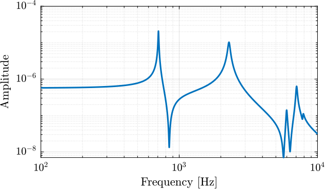
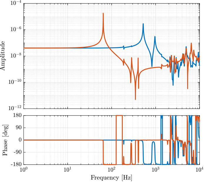
The resonance frequency is specified to be between 650Hz and 840Hz. This is also the case for the FEM model (Figure fig:apa300ml_resonance).
Amplification factor
The amplification factor is the ratio of the vertical displacement to the stack displacement.
The ratio of the two displacement is computed from the FEM model.
abs(dcgain(G(1,1))./dcgain(G(2,1)))5.0749
This is actually correct and approximately corresponds to the ratio of the piezo height and length:
75/155
Stroke
Estimation of the actuator stroke: \[ \Delta H = A n \Delta L \] with:
- $\Delta H$ Axial Stroke of the APA
- $A$ Amplification factor (5 for the APA300ML)
- $n$ Number of stack used
- $\Delta L$ Stroke of the stack (0.1% of its length)
1e6 * 5 * 3 * 20e-3 * 0.1e-2300
This is exactly the specified stroke in the data-sheet.
TODO Stroke BIS
- Identified the stroke form the transfer function from V to z
Identification of the Dynamics from actuator to replace displacement
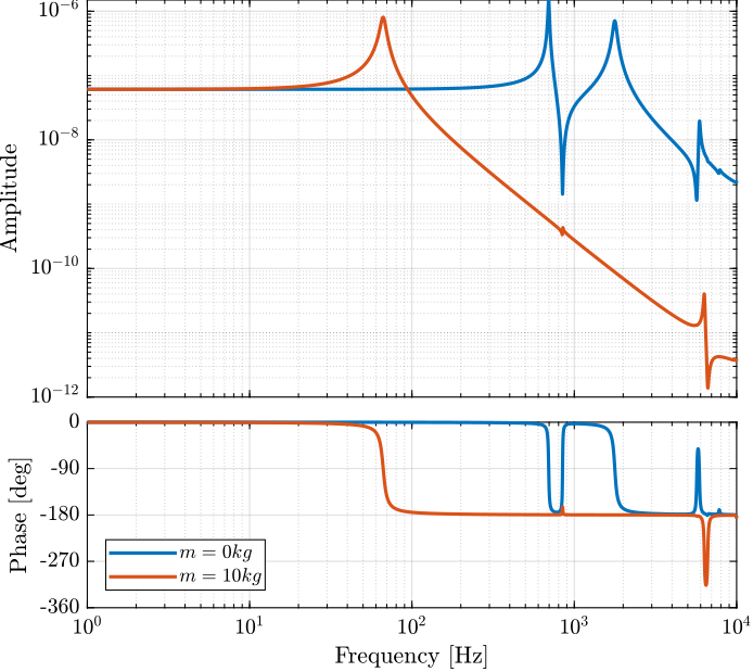
We first set the mass to be approximately zero.
The dynamics is identified from the applied force to the measured relative displacement.
The same dynamics is identified for a payload mass of 10Kg.
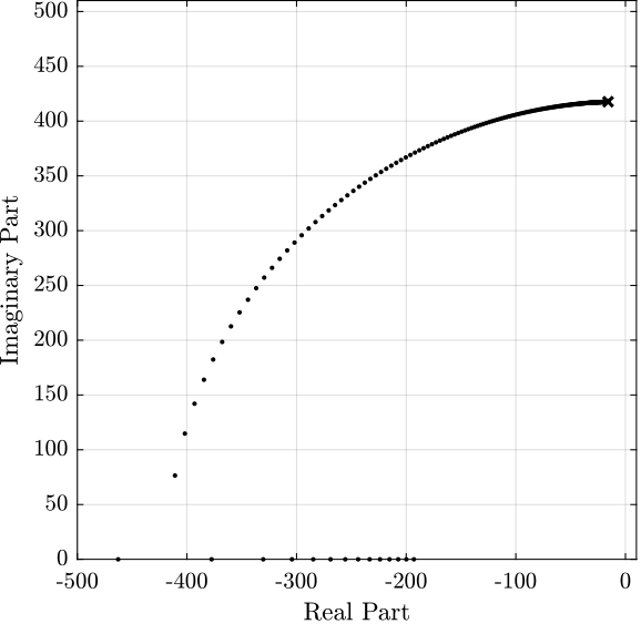
m = 10;The root locus corresponding to Direct Velocity Feedback with a mass of 10kg is shown in Figure fig:apa300ml_dvf_root_locus.
Identification of the Dynamics from actuator to force sensor
Let's use 2 stacks as a force sensor and 1 stack as force actuator.
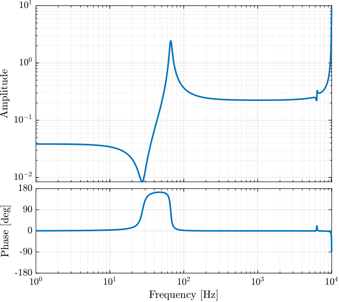
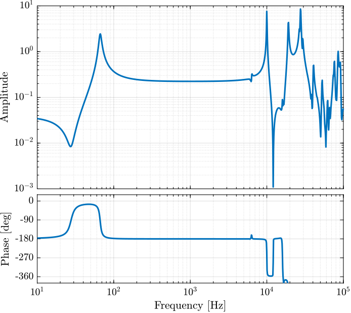
The transfer function from actuator voltage to sensor voltage is identified and shown in Figure fig:apa300ml_iff_plant.
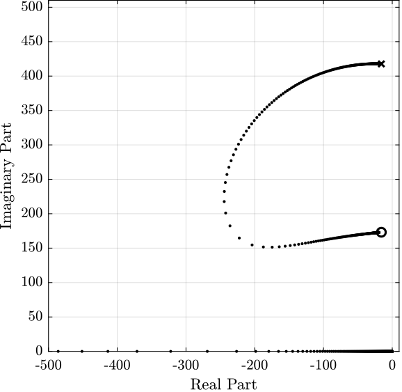
For root locus corresponding to IFF is shown in Figure fig:apa300ml_iff_root_locus.
Identification for a simpler model
The goal in this section is to identify the parameters of a simple APA model from the FEM. This can be useful is a lower order model is to be used for simulations.
The presented model is based on cite:souleille18_concep_activ_mount_space_applic.
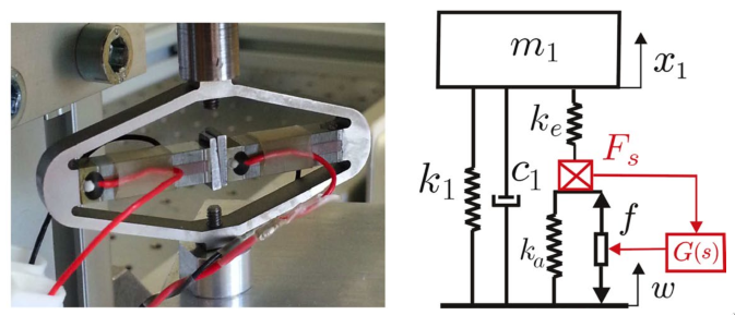
The model represents the Amplified Piezo Actuator (APA) from Cedrat-Technologies (Figure fig:souleille18_model_piezo). The parameters are shown in the table below.
#+caption:Parameters used for the model of the APA 100M
| Meaning | |
|---|---|
| $k_e$ | Stiffness used to adjust the pole of the isolator |
| $k_1$ | Stiffness of the metallic suspension when the stack is removed |
| $k_a$ | Stiffness of the actuator |
| $c_1$ | Added viscous damping |
The goal is to determine $k_e$, $k_a$ and $k_1$ so that the simplified model fits the FEM model.
\[ \alpha = \frac{x_1}{f}(\omega=0) = \frac{\frac{k_e}{k_e + k_a}}{k_1 + \frac{k_e k_a}{k_e + k_a}} \] \[ \beta = \frac{x_1}{F}(\omega=0) = \frac{1}{k_1 + \frac{k_e k_a}{k_e + k_a}} \]
If we can fix $k_a$, we can determine $k_e$ and $k_1$ with: \[ k_e = \frac{k_a}{\frac{\beta}{\alpha} - 1} \] \[ k_1 = \frac{1}{\beta} - \frac{k_e k_a}{k_e + k_a} \]
From the identified dynamics, compute $\alpha$ and $\beta$
  alpha = abs(dcgain(G('y', 'Fa')));
  beta  = abs(dcgain(G('y', 'Fd')));
$k_a$ is estimated using the following formula:
ka = 0.8/abs(dcgain(G('y', 'Fa')));The factor can be adjusted to better match the curves.
Then $k_e$ and $k_1$ are computed.
  ke = ka/(beta/alpha - 1);
  k1 = 1/beta - ke*ka/(ke + ka);
#+caption:Obtained stiffnesses of the APA 100M
| Value [N/um] | |
|---|---|
| ka | 40.5 |
| ke | 1.5 |
| k1 | 0.4 |
The damping in the system is adjusted to match the FEM model if necessary.
c1 = 1e2;The analytical model of the simpler system is defined below:
  Ga = 1/(m*s^2 + k1 + c1*s + ke*ka/(ke + ka)) * ...
       [ 1 ,              k1 + c1*s + ke*ka/(ke + ka)  , ke/(ke + ka) ;
        -ke*ka/(ke + ka), ke*ka/(ke + ka)*m*s^2 ,       -ke/(ke + ka)*(m*s^2 + c1*s + k1)];

  Ga.InputName = {'Fd', 'w', 'Fa'};
  Ga.OutputName = {'y', 'Fs'};
And the DC gain is adjusted for the force sensor:
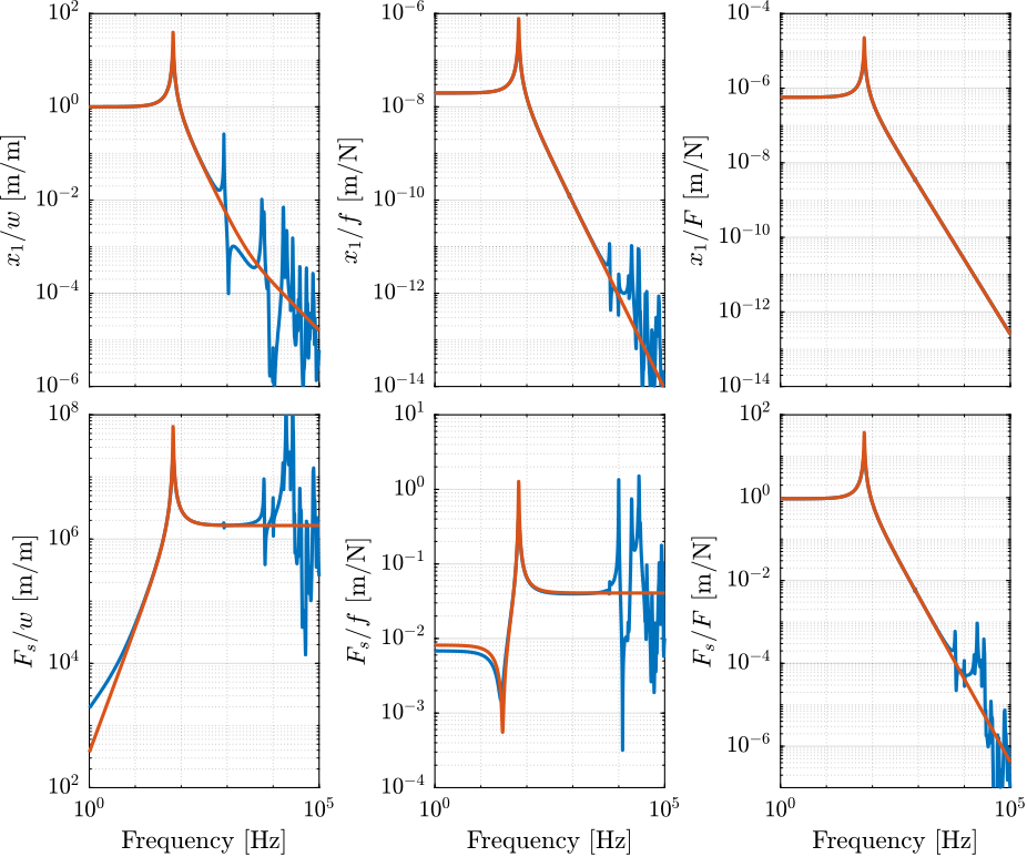
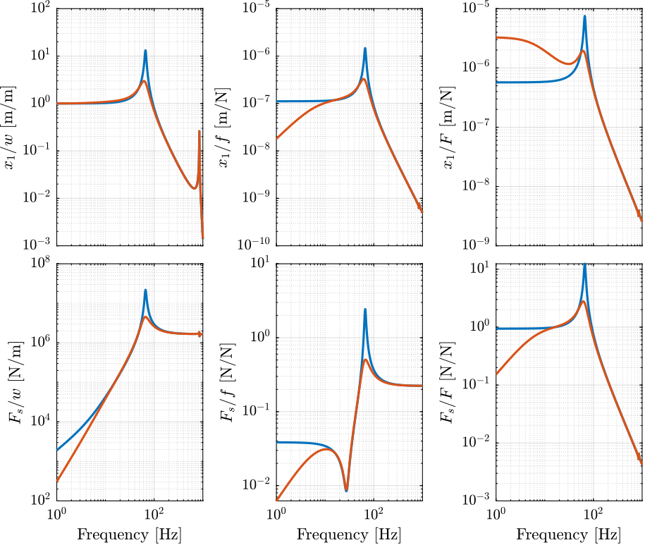
F_gain = dcgain(G('Fs', 'Fd'))/dcgain(Ga('Fs', 'Fd'));The dynamics of the FEM model and the simpler model are compared in Figure fig:apa300ml_comp_simpler_model.
The simplified model has also been implemented in Simscape.
The dynamics of the Simscape simplified model is identified and compared with the FEM one in Figure fig:apa300ml_comp_simpler_simscape.
Integral Force Feedback
In this section, Integral Force Feedback control architecture is applied on the APA300ML.
First, the plant (dynamics from voltage actuator to voltage sensor is identified).
The payload mass is set to 10kg.
m = 10;The obtained dynamics is shown in Figure fig:piezo_amplified_iff_plant.
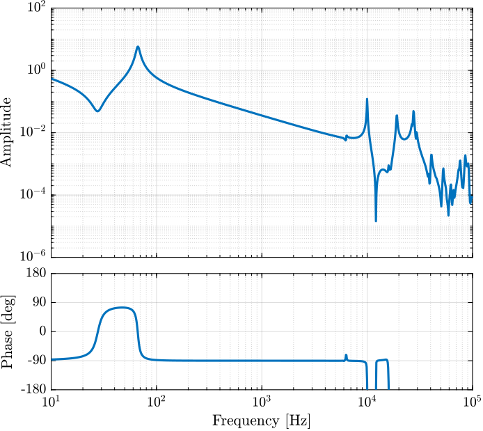
The controller is defined below and the loop gain is shown in Figure fig:piezo_amplified_iff_loop_gain.
Kiff = -1e3/s;Now the closed-loop system is identified again and compare with the open loop system in Figure fig:piezo_amplified_iff_comp.
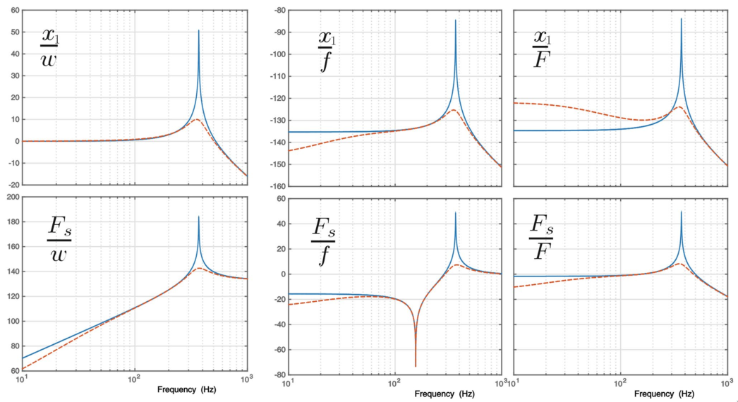
It is the expected behavior as shown in the Figure fig:souleille18_results (from cite:souleille18_concep_activ_mount_space_applic).
First Flexible Joint Geometry
<<sec:flexor_ID16>>
Introduction ignore
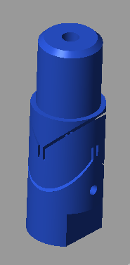
The studied flexor is shown in Figure fig:flexor_id16_screenshot.
The stiffness and mass matrices representing the dynamics of the flexor are exported from a FEM. It is then imported into Simscape.
A simplified model of the flexor is then developped.
Import Mass Matrix, Stiffness Matrix, and Interface Nodes Coordinates
We first extract the stiffness and mass matrices.
  K = extractMatrix('mat_K_6modes_2MDoF.matrix');
M = extractMatrix('mat_M_6modes_2MDoF.matrix');| 11200000 | 195 | 2220 | -0.719 | -265 | 1.59 | -11200000 | -213 | -2220 | 0.147 | 195 | 11400000 | 1290 | -148 | -0.188 | 2.41 | -212 | -11400000 | -1290 | 148 | |
| 2220 | 1290 | 119000000 | 1.31 | 1.49 | 1.79 | -2220 | -1290 | -119000000 | -1.31 | |||||||||||
| -0.719 | -148 | 1.31 | 33 | 000488 | -000977 | 0.141 | 148 | -1.31 | -33 | |||||||||||
| -265 | -0.188 | 1.49 | 000488 | 33 | 00293 | 266 | 0.154 | -1.49 | 00026 | |||||||||||
| 1.59 | 2.41 | 1.79 | -000977 | 00293 | 236 | -1.32 | -2.55 | -1.79 | 000379 | |||||||||||
| -11200000 | -212 | -2220 | 0.141 | 266 | -1.32 | 11400000 | 24600 | 1640 | 120 | |||||||||||
| -213 | -11400000 | -1290 | 148 | 0.154 | -2.55 | 24600 | 11400000 | 1290 | -72 | |||||||||||
| -2220 | -1290 | -119000000 | -1.31 | -1.49 | -1.79 | 1640 | 1290 | 119000000 | 1.32 | |||||||||||
| 0.147 | 148 | -1.31 | -33 | 00026 | 000379 | 120 | -72 | 1.32 | 34.7 |
| 0.02 | 1e-09 | -4e-08 | -1e-10 | 0.0002 | -3e-11 | 0.004 | 5e-08 | 7e-08 | 1e-10 |
| 1e-09 | 0.02 | -3e-07 | -0.0002 | -1e-10 | -2e-09 | 2e-08 | 0.004 | 3e-07 | 1e-05 |
| -4e-08 | -3e-07 | 0.02 | 7e-10 | -2e-09 | 1e-09 | 3e-07 | 7e-08 | 0.003 | 1e-09 |
| -1e-10 | -0.0002 | 7e-10 | 4e-06 | -1e-12 | -6e-13 | 2e-10 | -7e-06 | -8e-10 | -1e-09 |
| 0.0002 | -1e-10 | -2e-09 | -1e-12 | 3e-06 | 2e-13 | 9e-06 | 4e-11 | 2e-09 | -3e-13 |
| -3e-11 | -2e-09 | 1e-09 | -6e-13 | 2e-13 | 4e-07 | 8e-11 | 9e-10 | -1e-09 | 2e-12 |
| 0.004 | 2e-08 | 3e-07 | 2e-10 | 9e-06 | 8e-11 | 0.02 | -7e-08 | -3e-07 | -2e-10 |
| 5e-08 | 0.004 | 7e-08 | -7e-06 | 4e-11 | 9e-10 | -7e-08 | 0.01 | -4e-08 | 0.0002 |
| 7e-08 | 3e-07 | 0.003 | -8e-10 | 2e-09 | -1e-09 | -3e-07 | -4e-08 | 0.02 | -1e-09 |
| 1e-10 | 1e-05 | 1e-09 | -1e-09 | -3e-13 | 2e-12 | -2e-10 | 0.0002 | -1e-09 | 2e-06 |
| Total number of Nodes | 2 |
| Number of interface Nodes | 2 |
| Number of Modes | 6 |
| Size of M and K matrices | 18 |
Then, we extract the coordinates of the interface nodes.
[int_xyz, int_i, n_xyz, n_i, nodes] = extractNodes('out_nodes_3D.txt');| Node i | Node Number | x [m] | y [m] | z [m] |
|---|---|---|---|---|
| 1.0 | 181278.0 | 0.0 | 0.0 | 0.0 |
| 2.0 | 181279.0 | 0.0 | 0.0 | -0.0 |
Using K, M and int_xyz, we can use the Reduced Order Flexible Solid simscape block.
Identification of the parameters using Simscape and looking at the Stiffness Matrix
The flexor is now imported into Simscape and its parameters are estimated using an identification.
The dynamics is identified from the applied force/torque to the measured displacement/rotation of the flexor.
And we find the same parameters as the one estimated from the Stiffness matrix.
| Characteristic | Value | Identification |
|---|---|---|
| Axial Stiffness Dz [N/um] | 119 | 119 |
| Bending Stiffness Rx [Nm/rad] | 33 | 33 |
| Bending Stiffness Ry [Nm/rad] | 33 | 33 |
| Torsion Stiffness Rz [Nm/rad] | 236 | 236 |
Simpler Model
Let's now model the flexible joint with a "perfect" Bushing joint as shown in Figure fig:flexible_joint_simscape.
The parameters of the Bushing joint (stiffnesses) are estimated from the Stiffness matrix that was computed from the FEM.
  Kx = K(1,1); % [N/m]
  Ky = K(2,2); % [N/m]
  Kz = K(3,3); % [N/m]
  Krx = K(4,4); % [Nm/rad]
  Kry = K(5,5); % [Nm/rad]
  Krz =  K(6,6); % [Nm/rad]
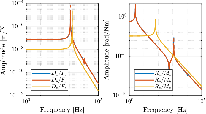
The dynamics from the applied force/torque to the measured displacement/rotation of the flexor is identified again for this simpler model.
The two obtained dynamics are compared in Figure
Optimized Flexible Joint
<<sec:flexor_025>>
Introduction ignore
The joint geometry has been optimized using Ansys to have lower bending stiffness while keeping a large axial stiffness.
The obtained geometry is shown in Figure fig:optimal_flexor.
Import Mass Matrix, Stiffness Matrix, and Interface Nodes Coordinates
We first extract the stiffness and mass matrices.
  K = readmatrix('flex025_mat_K.CSV');
M = readmatrix('flex025_mat_M.CSV');| 12700000 | -18.5 | -26.8 | 00162 | -4.63 | 64 | -12700000 | 18.3 | 26.7 | 00234 |
| -18.5 | 12700000 | -499 | -132 | 00414 | -0.495 | 18.4 | -12700000 | 499 | 132 |
| -26.8 | -499 | 94000000 | -470 | 00771 | -0.855 | 26.8 | 498 | -94000000 | 470 |
| 00162 | -132 | -470 | 4.83 | 2.61e-07 | 000123 | -00163 | 132 | 470 | -4.83 |
| -4.63 | 00414 | 00771 | 2.61e-07 | 4.83 | 4.43e-05 | 4.63 | -00413 | -00772 | -4.3e-07 |
| 64 | -0.495 | -0.855 | 000123 | 4.43e-05 | 260 | -64 | 0.495 | 0.855 | -000124 |
| -12700000 | 18.4 | 26.8 | -00163 | 4.63 | -64 | 12700000 | -18.2 | -26.7 | -00234 |
| 18.3 | -12700000 | 498 | 132 | -00413 | 0.495 | -18.2 | 12700000 | -498 | -132 |
| 26.7 | 499 | -94000000 | 470 | -00772 | 0.855 | -26.7 | -498 | 94000000 | -470 |
| 00234 | 132 | 470 | -4.83 | -4.3e-07 | -000124 | -00234 | -132 | -470 | 4.83 |
| 0.006 | 8e-09 | -2e-08 | -1e-10 | 3e-05 | 3e-08 | 0.003 | -3e-09 | 9e-09 | 2e-12 |
| 8e-09 | 0.02 | 1e-07 | -3e-05 | 1e-11 | 6e-10 | 1e-08 | 0.003 | -5e-08 | 3e-09 |
| -2e-08 | 1e-07 | 0.01 | -6e-08 | -6e-11 | -8e-12 | -1e-07 | 1e-08 | 0.003 | -1e-08 |
| -1e-10 | -3e-05 | -6e-08 | 1e-06 | 7e-14 | 6e-13 | 1e-10 | 1e-06 | -1e-08 | 3e-10 |
| 3e-05 | 1e-11 | -6e-11 | 7e-14 | 2e-07 | 1e-10 | 3e-08 | -7e-12 | 6e-11 | -6e-16 |
| 3e-08 | 6e-10 | -8e-12 | 6e-13 | 1e-10 | 5e-07 | 1e-08 | -5e-10 | -1e-11 | 1e-13 |
| 0.003 | 1e-08 | -1e-07 | 1e-10 | 3e-08 | 1e-08 | 0.02 | -2e-08 | 1e-07 | -4e-12 |
| -3e-09 | 0.003 | 1e-08 | 1e-06 | -7e-12 | -5e-10 | -2e-08 | 0.006 | -8e-08 | 3e-05 |
| 9e-09 | -5e-08 | 0.003 | -1e-08 | 6e-11 | -1e-11 | 1e-07 | -8e-08 | 0.01 | -6e-08 |
| 2e-12 | 3e-09 | -1e-08 | 3e-10 | -6e-16 | 1e-13 | -4e-12 | 3e-05 | -6e-08 | 2e-07 |
Then, we extract the coordinates of the interface nodes.
[int_xyz, int_i, n_xyz, n_i, nodes] = extractNodes('flex025_out_nodes_3D.txt');| Total number of Nodes | 2 |
| Number of interface Nodes | 2 |
| Number of Modes | 6 |
| Size of M and K matrices | 18 |
| Node i | Node Number | x [m] | y [m] | z [m] |
|---|---|---|---|---|
| 1.0 | 528875.0 | 0.0 | 0.0 | 0.0 |
| 2.0 | 528876.0 | 0.0 | 0.0 | -0.0 |
Using K, M and int_xyz, we can use the Reduced Order Flexible Solid simscape block.
Identification of the parameters using Simscape
The flexor is now imported into Simscape and its parameters are estimated using an identification.
The dynamics is identified from the applied force/torque to the measured displacement/rotation of the flexor.
And we find the same parameters as the one estimated from the Stiffness matrix.
| Caracteristic | Value | Identification |
|---|---|---|
| Axial Stiffness Dz [N/um] | 94.0 | 93.9 |
| Bending Stiffness Rx [Nm/rad] | 4.8 | 4.8 |
| Bending Stiffness Ry [Nm/rad] | 4.8 | 4.8 |
| Torsion Stiffness Rz [Nm/rad] | 260.2 | 260.2 |
Simpler Model
Let's now model the flexible joint with a "perfect" Bushing joint as shown in Figure fig:flexible_joint_simscape.
The parameters of the Bushing joint (stiffnesses) are estimated from the Stiffness matrix that was computed from the FEM.
  Kx = K(1,1); % [N/m]
  Ky = K(2,2); % [N/m]
  Kz = K(3,3); % [N/m]
  Krx = K(4,4); % [Nm/rad]
  Kry = K(5,5); % [Nm/rad]
  Krz =  K(6,6); % [Nm/rad]
The dynamics from the applied force/torque to the measured displacement/rotation of the flexor is identified again for this simpler model.
The two obtained dynamics are compared in Figure
Comparison with a stiffer Flexible Joint
The stiffness matrix with the flexible joint with a "hinge" size of 0.50mm is loaded.
K_050 = readmatrix('flex050_mat_K.CSV');Its parameters are compared with the Flexible Joint with a size of 0.25mm in the table below.
| Caracteristic | 0.25 mm | 0.50 mm |
|---|---|---|
| Axial Stiffness Dz [N/um] | 94.0 | 124.7 |
| Shear Stiffness [N/um] | 12.7 | 25.8 |
| Bending Stiffness Rx [Nm/rad] | 4.8 | 26.0 |
| Bending Stiffness Ry [Nm/rad] | 4.8 | 26.0 |
| Torsion Stiffness Rz [Nm/rad] | 260.2 | 538.0 |
Complete Strut with Encoder
<<sec:strut_encoder>>
Introduction
Now, the full nano-hexapod strut is modelled using Ansys.
The 3D as well as the interface nodes are shown in Figure fig:strut_encoder_points3.
A side view is shown in Figure fig:strut_encoder_nodes_side.
The flexible joints used have a 0.25mm width size.
Import Mass Matrix, Stiffness Matrix, and Interface Nodes Coordinates
We first extract the stiffness and mass matrices.
  K = readmatrix('strut_encoder_mat_K.CSV');
M = readmatrix('strut_encoder_mat_M.CSV');| 2000000 | 1000000 | -3000000 | -400 | 300 | 200 | -30 | 2000 | -10000 | 0.3 |
| 1000000 | 4000000 | -8000000 | -900 | 400 | -50 | -6000 | 10000 | -20000 | 3 |
| -3000000 | -8000000 | 20000000 | 2000 | -900 | 200 | -10000 | 20000 | -300000 | 7 |
| -400 | -900 | 2000 | 5 | -0.1 | 05 | 1 | -3 | 6 | -0007 |
| 300 | 400 | -900 | -0.1 | 5 | 04 | -0.1 | 0.5 | -3 | 0001 |
| 200 | -50 | 200 | 05 | 04 | 300 | 4 | -01 | -1 | 3e-05 |
| -30 | -6000 | -10000 | 1 | -0.1 | 4 | 3000000 | -1000000 | -2000000 | -300 |
| 2000 | 10000 | 20000 | -3 | 0.5 | -01 | -1000000 | 6000000 | 7000000 | 1000 |
| -10000 | -20000 | -300000 | 6 | -3 | -1 | -2000000 | 7000000 | 20000000 | 2000 |
| 0.3 | 3 | 7 | -0007 | 0001 | 3e-05 | -300 | 1000 | 2000 | 5 |
| 0.04 | -0.005 | 0.007 | 2e-06 | 0.0001 | -5e-07 | -1e-05 | -9e-07 | 8e-05 | -5e-10 |
| -0.005 | 0.03 | 0.02 | -0.0001 | 1e-06 | -3e-07 | 3e-05 | -0.0001 | 8e-05 | -3e-08 |
| 0.007 | 0.02 | 0.08 | -6e-06 | -5e-06 | -7e-07 | 4e-05 | -0.0001 | 0.0005 | -3e-08 |
| 2e-06 | -0.0001 | -6e-06 | 2e-06 | -4e-10 | 2e-11 | -8e-09 | 3e-08 | -2e-08 | 6e-12 |
| 0.0001 | 1e-06 | -5e-06 | -4e-10 | 3e-06 | 2e-10 | -3e-09 | 3e-09 | -7e-09 | 6e-13 |
| -5e-07 | -3e-07 | -7e-07 | 2e-11 | 2e-10 | 5e-07 | -2e-08 | 5e-09 | -5e-09 | 1e-12 |
| -1e-05 | 3e-05 | 4e-05 | -8e-09 | -3e-09 | -2e-08 | 0.04 | 0.004 | 0.003 | 1e-06 |
| -9e-07 | -0.0001 | -0.0001 | 3e-08 | 3e-09 | 5e-09 | 0.004 | 0.02 | -0.02 | 0.0001 |
| 8e-05 | 8e-05 | 0.0005 | -2e-08 | -7e-09 | -5e-09 | 0.003 | -0.02 | 0.08 | -5e-06 |
| -5e-10 | -3e-08 | -3e-08 | 6e-12 | 6e-13 | 1e-12 | 1e-06 | 0.0001 | -5e-06 | 2e-06 |
Then, we extract the coordinates of the interface nodes.
[int_xyz, int_i, n_xyz, n_i, nodes] = extractNodes('strut_encoder_out_nodes_3D.txt');| Total number of Nodes | 8 |
| Number of interface Nodes | 8 |
| Number of Modes | 6 |
| Size of M and K matrices | 54 |
| Node i | Node Number | x [m] | y [m] | z [m] |
|---|---|---|---|---|
| 1.0 | 504411.0 | 0.0 | 0.0 | 0.0405 |
| 2.0 | 504412.0 | 0.0 | 0.0 | -0.0405 |
| 3.0 | 504413.0 | -0.0325 | 0.0 | 0.0 |
| 4.0 | 504414.0 | -0.0125 | 0.0 | 0.0 |
| 5.0 | 504415.0 | -0.0075 | 0.0 | 0.0 |
| 6.0 | 504416.0 | 0.0325 | 0.0 | 0.0 |
| 7.0 | 504417.0 | 0.004 | 0.0145 | -0.00175 |
| 8.0 | 504418.0 | 0.004 | 0.0166 | -0.00175 |
Using K, M and int_xyz, we can use the Reduced Order Flexible Solid simscape block.
Piezoelectric parameters
Parameters for the APA300ML:
  d33 = 300e-12; % Strain constant [m/V]
  n   = 80;      % Number of layers per stack
  eT  = 1.6e-8;  % Permittivity under constant stress [F/m]
  sD  = 1e-11;   % Compliance under constant electric displacement [m2/N]
  ka  = 235e6;   % Stack stiffness [N/m]
  C   = 5e-6;    % Stack capactiance [F]
na = 2; % Number of stacks used as actuator
ns = 1; % Number of stacks used as force sensor