lecture-h-infinity/index.org

Robust Control - $\mathcal{H}_\infty$ Synthesis

• Introduction
• Introduction to the Control Methodology - Model Based Control
  • Control Methodology
  • Some Background: From Classical Control to Robust Control
  • Example System
• Classical Open Loop Shaping
  • Introduction to Open Loop Shaping
  • Example of Open Loop Shaping
  • $\mathcal{H}_\infty$ Loop Shaping Synthesis
  • Example of the $\mathcal{H}_\infty$ Loop Shaping Synthesis
• First Step in the $\mathcal{H}_\infty$ world
  • The $\mathcal{H}_\infty$ Norm
  • $\mathcal{H}_\infty$ Synthesis
  • The Generalized Plant
  • From a Classical Feedback Architecture to a Generalized Plant
  • The General Synthesis Problem Formulation
• Modern Interpretation of the Control Specifications
  • Introduction
• Resources

TODO Introduction   ignore

Introduction to the Control Methodology - Model Based Control

Control Methodology

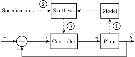
The typical methodology when applying Model Based Control to a plant is schematically shown in Figure fig:control-procedure. It consists of three steps:

1. Identification or modeling: $\Longrightarrow$ mathematical model

2. Translate the specifications into mathematical criteria:

   • Specifications: Response Time, Noise Rejection, Maximum input amplitude, Robustness, …
   • Mathematical Criteria: Cost Function, Shape of TF
3. Synthesis: research of $K$ that satisfies the specifications for the model of the system

  \begin{tikzpicture}
    \node[addb={+}{}{}{}{-}] (addsub) at (0, 0){};

    \node[block, right=1.5 of addsub] (controller) {Controller};
    \node[block, right=1.5 of controller] (plant) {Plant};

    \node[block, above=1 of controller] (controller_design) {Synthesis};
    \node[block, above=1 of plant] (model_plant) {Model};

    \draw[<-] (addsub.west) -- ++(-1, 0) node[above right]{$r$};

    \draw[->] (addsub) -- (controller.west) node[above left]{$\epsilon$};
    \draw[->] (controller) -- (plant.west) node[above left]{$u$};
    \draw[->] (plant.east) -- ++(1, 0) node[above left]{$y$};
    \draw[] ($(plant.east) + (0.5, 0)$) -- ++(0, -1);
    \draw[->] ($(plant.east) + (0.5, -1)$) -| (addsub.south);

    \draw[->, dashed] (plant) -- node[midway, right, labelc, solid]{1} (model_plant);
    \draw[->, dashed] (controller_design) --node[midway, right, labelc, solid]{3} (controller);
    \draw[->, dashed] (model_plant) -- (controller_design);
    \draw[<-, dashed] (controller_design.west) -- node[midway, above, labelc, solid]{2} ++(-1, 0) node[left, style={align=center}]{Specifications};
  \end{tikzpicture}

Typical Methodoly for Model Based Control

In this document, we will mainly focus on steps 2 and 3.

Some Background: From Classical Control to Robust Control

	Classical Control	Modern Control	Robust Control
Date	1930-	1960-	1980-
Tools	Transfer Functions	State Space formulation	Systems and Signals Norms ($\mathcal{H}_\infty$, $\mathcal{H}_2$ Norms)
	Nyquist Plots	Riccati Equations	Closed Loop Transfer Functions
	Bode Plots		Open/Closed Loop Shaping
	Phase and Gain margins		Weighting Functions
			Disk margin
Control Architectures	Proportional, Integral, Derivative	Full State Feedback	General Control Configuration
	Leads, Lags	LQR, LQG
		Kalman Filters
Advantages	Study Stability	Automatic Synthesis	Automatic Synthesis
	Simple	MIMO	MIMO
	Natural	Optimization Problem	Optimization Problem
			Guaranteed Robustness
			Easy specification of performances
Disadvantages	Manual Method	No Guaranteed Robustness	Required knowledge of specific tools
	Only SISO	Difficult Rejection of Perturbations	Need a reasonably good model of the system

Table summurazing the main differences between classical, modern and robust control

Example System

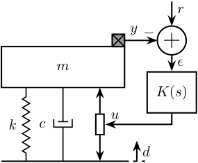
Let's consider the model shown in Figure fig:mech_sys_1dof_inertial_contr. It could represent a suspension system with a payload to position or isolate using an force actuator and an inertial sensor. The notations used are listed in Table tab:example_notations.

  \begin{tikzpicture}
    % Parameters
    \def\massw{3}
    \def\massh{1}
    \def\spaceh{1.8}

    % Ground
    \draw[] (-0.5*\massw, 0) -- (0.5*\massw, 0);
    % Mass
    \draw[fill=white] (-0.5*\massw, \spaceh) rectangle (0.5*\massw, \spaceh+\massh) node[pos=0.5](m){$m$};

    % Spring, Damper, and Actuator
    \draw[spring]   (-0.3*\massw, 0) -- (-0.3*\massw, \spaceh) node[midway, left=0.1]{$k$};
    \draw[damper]   ( 0, 0) -- ( 0, \spaceh) node[midway, left=0.3]{$c$};
    \draw[actuator] ( 0.3*\massw, 0) -- (0.3*\massw, \spaceh) node[midway](F){};

    % Displacements
    \draw[dashed] (0.5*\massw, 0) -- ++(0.5, 0);
    \draw[->] (0.6*\massw, 0) -- ++(0, 0.5) node[below right]{$d$};

    % Inertial Sensor
    \node[inertialsensor] (inertials) at (0.5*\massw, \spaceh+\massh){};
    \node[addb={+}{-}{}{}{}, right=0.8 of inertials] (subf) {};

    \node[block, below=0.4 of subf] (K){$K(s)$};

    \draw[->] (inertials.east) node[above right]{$y$} -- (subf.west);
    \draw[->] (subf.south) -- (K.north) node[above right]{$\epsilon$};
    \draw[<-] (subf.north) -- ++(0, 0.6) node[below right]{$r$};
    \draw[->] (K.south) |- (F.east) node[above right]{$u$};
  \end{tikzpicture}

Test System consisting of a payload with a mass $m$ on top of an active system with a stiffness $k$, damping $c$ and an actuator. A feedback controller $K(s)$ is added to position / isolate the payload.

Notation	Description	Value	Unit
$m$	Payload's mass to position / isolate	$10$	[kg]
$k$	Stiffness of the suspension system	$10^6$	[N/m]
$c$	Damping coefficient of the suspension system	$400$	[N/(m/s)]
$y$	Payload absolute displacement (measured by an inertial sensor)		[m]
$d$	Ground displacement, it acts as a disturbance		[m]
$u$	Actuator force		[N]
$r$	Wanted position of the mass (the reference)		[m]
$\epsilon = r - y$	Position error		[m]
$K$	Feedback controller	to be designed	[N/m]

Example system variables

Derive the following open-loop transfer functions:

\begin{align} G(s) &= \frac{y}{u} \\ G_d(s) &= \frac{y}{d} \end{align}

Hint

You can follow this generic procedure:

1. List all applied forces ot the mass: Actuator force, Stiffness force (Hooke's law), …
2. Apply the Newton's Second Law on the payload \[ m \ddot{y} = \Sigma F \]
3. Transform the differential equations into the Laplace domain: \[ \frac{d\ \cdot}{dt} \Leftrightarrow \cdot \times s \]
4. Write $y(s)$ as a function of $u(s)$ and $w(s)$

Results

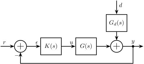
\begin{align} G(s) &= \frac{1}{m s^2 + cs + k} \\ G_d(s) &= \frac{cs + k}{m s^2 + cs + k} \end{align}

Having obtained $G(s)$ and $G_d(s)$, we can transform the system shown in Figure fig:mech_sys_1dof_inertial_contr into a classical feedback form as shown in Figure fig:open_loop_shaping.

  \begin{tikzpicture}
    \node[addb={+}{}{}{}{-}] (addfb) at (0, 0){};
    \node[block, right=0.8 of addfb] (K){$K(s)$};
    \node[block, right=0.8 of K] (G){$G(s)$};
    \node[addb={+}{}{}{}{}, right=0.8 of G] (addd){};
    \node[block, above=0.5 of addd] (Gd){$G_d(s)$};

    \draw[<-] (addfb.west) -- ++(-0.8, 0) node[above right]{$r$};
    \draw[->] (addfb.east) -- (K.west) node[above left]{$\epsilon$};
    \draw[->] (K.east) -- (G.west) node[above left]{$u$};
    \draw[->] (G.east) -- (addd.west);
    \draw[<-] (Gd.north) -- ++(0, 0.8) node[below right]{$d$};
    \draw[->] (Gd.south) -- (addd.north);
    \draw[->] (addd.east) -- ++(1.2, 0);
    \draw[->] ($(addd.east) + (0.6, 0)$) node[branch]{} node[above]{$y$} -- ++(0, -1.0) -| (addfb.south);
  \end{tikzpicture}

Block diagram corresponding to the example system

Let's define the system parameters on Matlab.

  k = 1e6; % Stiffness [N/m]
  c = 4e2; % Damping [N/(m/s)]
  m = 10; % Mass [kg]

And now the system dynamics $G(s)$ and $G_d(s)$ (their bode plots are shown in Figures fig:bode_plot_example_afm and fig:bode_plot_example_Gd).

  G = 1/(m*s^2 + c*s + k); % Plant
  Gd = (c*s + k)/(m*s^2 + c*s + k); % Disturbance

Bode plot of the plant $G(s)$

Magnitude of the disturbance transfer function $G_d(s)$

Classical Open Loop Shaping

Introduction to Open Loop Shaping

The Loop Gain $L(s)$ usually refers to as the product of the controller and the plant (Figure fig:open_loop_shaping):

\begin{equation} L(s) = G(s) \cdot K(s) \label{eq:loop_gain} \end{equation}

  \begin{tikzpicture}
    \node[addb={+}{}{}{}{-}] (addsub) at (0, 0){};

    \node[block, right=0.8 of addsub] (K) {$K(s)$};
    \node[below] at (K.south) {Controller};
    \node[block, right=0.8 of K] (G) {$G(s)$};
    \node[below] at (G.south) {Plant};

    \draw[<-] (addsub.west) -- ++(-0.8, 0) node[above right]{$r$};

    \draw[->] (addsub) -- (K.west) node[above left]{$\epsilon$};
    \draw[->] (K.east) -- (G.west) node[above left]{$u$};
    \draw[->] (G.east) -- ++(0.8, 0) node[above left]{$y$};
    \draw[] ($(G.east) + (0.5, 0)$) -- ++(0, -1.4);
    \draw[->] ($(G.east) + (0.5, -1.4)$) -| (addsub.south);

    \draw [decoration={brace, raise=5pt}, decorate] (K.north west) -- node[above=6pt]{$L(s)$} (G.north east);
  \end{tikzpicture}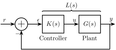

Classical Feedback Architecture

Open Loop Shaping refers to a control design technique where the controller $K(s)$ is designed such that the Open Loop Gain $L(s)$ has desirable shape.

This synthesis method is widely used as many characteristics of the closed-loop system depend on the shape of the open loop gain $L(s)$:

• Performance: $L$ large
• Good disturbance rejection: $L$ large
• Limitation of measurement noise on plant output: $L$ small
• Small magnitude of input signal: $K$ and $L$ small
• Nominal stability: $L$ small (RHP zeros and time delays)
• Robust stability: $L$ small (neglected dynamics)

The Open Loop shape is usually done manually has the loop gain $L(s)$ depends linearly on $K(s)$ eqref:eq:loop_gain.

$K(s)$ then consists of a combination of leads, lags, notches, etc. such that $L(s)$ has the wanted shape.

Example of Open Loop Shaping

Let's take our example system and try to apply the Open-Loop shaping strategy to design a controller that fulfils the following specifications:

• Performance: Bandwidth of approximately 10Hz
• Noise Attenuation: Roll-off of -40dB/decade past 30Hz
• Robustness: Gain margin > 3dB and Phase margin > 30 deg

Using SISOTOOL, design a controller that fulfill the specifications.

  sisotool(G)

In order to have the wanted Roll-off, two integrators are used, a lead is also added to have sufficient phase margin.

The obtained controller is shown below, and the bode plot of the Loop Gain is shown in Figure fig:loop_gain_manual_afm.

  K = 14e8 * ... % Gain
      1/(s^2) * ... % Double Integrator
      1/(1 + s/2/pi/40) * ... % Low Pass Filter
      (1 + s/(2*pi*10/sqrt(8)))/(1 + s/(2*pi*10*sqrt(8))); % Lead

Bode Plot of the obtained Loop Gain $L(s) = G(s) K(s)$

And we can verify that we have the wanted stability margins:

  [Gm, Pm, ~, Wc] = margin(G*K)

	Manual Method
Gain Margin $> 3$ [dB]	3.1
Phase Margin $> 30$ [deg]	35.4
Crossover $\approx 10$ [Hz]	10.1

$\mathcal{H}_\infty$ Loop Shaping Synthesis

The Open Loop Shaping synthesis can be performed using the $\mathcal{H}_\infty$ Synthesis.

Even though we will not go into details, we will provide one example.

Using Matlab, the $\mathcal{H}_\infty$ synthesis of a controller based on the wanted open loop shape can be performed using the loopsyn command:

  K = loopsyn(G, Gd);

where:

• G is the (LTI) plant
• Gd is the wanted loop shape
• K is the synthesize controller

Matlab documentation of loopsyn (link).

Example of the $\mathcal{H}_\infty$ Loop Shaping Synthesis

Let's reuse the previous plant.

Translate the specification into the wanted shape of the open loop gain.

• Performance: Bandwidth of approximately 10Hz: $|L_w(j2 \pi 10)| = 1$
• Noise Attenuation: Roll-off of -40dB/decade past 30Hz
• Robustness: Gain margin > 3dB and Phase margin > 30 deg

  Lw = 2.3e3 * ...
       1/(s^2) * ... % Double Integrator
       (1 + s/(2*pi*10/sqrt(3)))/(1 + s/(2*pi*10*sqrt(3))); % Lead

The $\mathcal{H}_\infty$ optimal open loop shaping is performed using the loopsyn command:

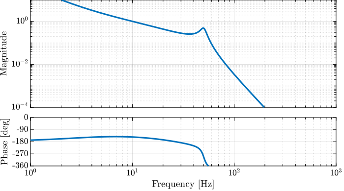
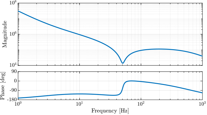
  [K, ~, GAM] = loopsyn(G, Lw);

The Bode plot of the obtained controller is shown in Figure fig:open_loop_shaping_hinf_K.

It is always important to analyze the controller after the synthesis is performed.

In the end, a synthesize controller is just a combination of low pass filters, high pass filters, notches, leads, etc.

Let's briefly analyze this controller:

• two integrators are used at low frequency to have the wanted low frequency high gain
• a lead is added centered with the crossover frequency to increase the phase margin
• a notch is added at the resonance of the plant to increase the gain margin (this is very typical of $\mathcal{H}_\infty$ controllers, and can be an issue, more info on that latter)

Obtained controller $K$ using the open-loop $\mathcal{H}_\infty$ shaping

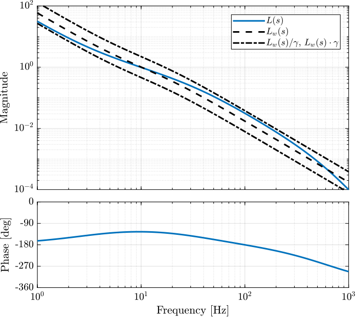
The obtained Loop Gain is shown in Figure fig:open_loop_shaping_hinf_L.

Obtained Open Loop Gain $L(s) = G(s) K(s)$ and comparison with the wanted Loop gain $L_w$

Let's now compare the obtained stability margins of the $\mathcal{H}_\infty$ controller and of the manually developed controller in Table tab:open_loop_shaping_compare.

Specifications	Manual Method	$\mathcal{H}_\infty$ Method
Gain Margin $> 3$ [dB]	3.1	31.7
Phase Margin $> 30$ [deg]	35.4	54.7
Crossover $\approx 10$ [Hz]	10.1	9.9

Comparison of the characteristics obtained with the two methods

First Step in the $\mathcal{H}_\infty$ world

The $\mathcal{H}_\infty$ Norm

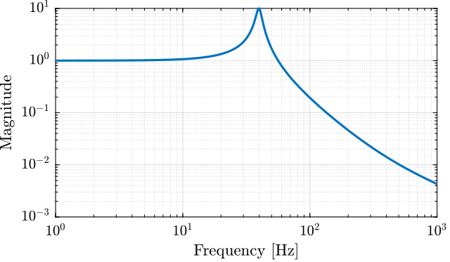
The $\mathcal{H}_\infty$ norm is defined as the peak of the maximum singular value of the frequency response

\begin{equation} \|G(s)\|_\infty = \max_\omega \bar{\sigma}\big( G(j\omega) \big) \end{equation}

For a SISO system $G(s)$, it is simply the peak value of $|G(j\omega)|$ as a function of frequency:

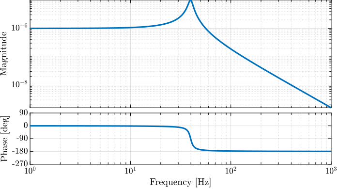
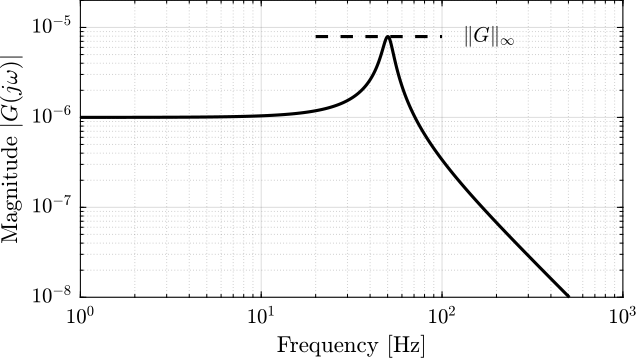
\begin{equation} \|G(s)\|_\infty = \max_{\omega} |G(j\omega)| \label{eq:hinf_norm_siso} \end{equation}

And compute its $\mathcal{H}_\infty$ norm using the hinfnorm function:

  hinfnorm(G)

7.9216e-06

The magnitude $|G(j\omega)|$ of the plant $G(s)$ as a function of frequency is shown in Figure fig:hinfinity_norm_siso_bode. The maximum value of the magnitude over all frequencies does correspond to the $\mathcal{H}_\infty$ norm of $G(s)$ as Equation eqref:eq:hinf_norm_siso implies.

Example of the $\mathcal{H}_\infty$ norm of a SISO system

$\mathcal{H}_\infty$ Synthesis

Optimization problem: $\mathcal{H}_\infty$ synthesis is a method that uses an algorithm (LMI optimization, Riccati equation) to find a controller of the same order as the system so that the $\mathcal{H}_\infty$ norms of defined transfer functions are minimized.

Engineer work:

1. Write the problem as standard $\mathcal{H}_\infty$ problem
2. Translate the specifications as $\mathcal{H}_\infty$ norms
3. Make the synthesis and analyze the obtain controller
4. Reduce the order of the controller for implementation

Many ways to use the $\mathcal{H}_\infty$ Synthesis:

• Traditional $\mathcal{H}_\infty$ Synthesis
• Mixed Sensitivity Loop Shaping
• Fixed-Structure $\mathcal{H}_\infty$ Synthesis
• Signal Based $\mathcal{H}_\infty$ Synthesis

The Generalized Plant

  \begin{tikzpicture}
    \node[block={2.0cm}{2.0cm}] (P) {$P$};
    \node[above] at (P.north) {Generalized Plant};

    % Input and outputs coordinates
    \coordinate[] (inputw)  at ($(P.south west)!0.75!(P.north west)$);
    \coordinate[] (inputu)  at ($(P.south west)!0.25!(P.north west)$);
    \coordinate[] (outputz) at ($(P.south east)!0.75!(P.north east)$);
    \coordinate[] (outputv) at ($(P.south east)!0.25!(P.north east)$);

    % Connections and labels
    \draw[<-] (inputw) -- ++(-0.8, 0) node[above right]{$w$};
    \draw[<-] (inputu) -- ++(-0.8, 0) node[above right]{$u$};

    \draw[->] (outputz) -- ++(0.8, 0) node[above left]{$z$};
    \draw[->] (outputv) -- ++(0.8, 0) node[above left]{$v$};
  \end{tikzpicture}

Notation	Meaning
$P$	Generalized plant model
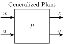
$w$	Exogenous inputs: commands, disturbances, noise
$z$	Exogenous outputs: signals to be minimized
$v$	Controller inputs: measurements
$u$	Control signals

Notations for the general configuration

\begin{equation} \begin{bmatrix} z \\ v \end{bmatrix} = P \begin{bmatrix} w \\ u \end{bmatrix} = \begin{bmatrix} P_{11} & P_{12} \\ P_{21} & P_{22} \end{bmatrix} \begin{bmatrix} w \\ u \end{bmatrix} \end{equation}

From a Classical Feedback Architecture to a Generalized Plant

  \begin{tikzpicture}
    \node[addb={+}{}{}{}{-}] (addfb) at (0, 0){};
    \node[block, right=0.8 of addfb] (K){$K(s)$};
    \node[addb={+}{}{}{}{}, right=0.8 of K] (addu){};
    \node[block, right=0.8 of addu] (G){$G(s)$};

    \draw[<-] (addfb.west) -- ++(-0.8, 0) node[above right]{$r$};
    \draw[->] (addfb.east) -- (K.west) node[above left]{$\epsilon$};
    \draw[->] (K.east) -- (addu.west) node[above left]{$u$};
    \draw[->] (addu.east) -- (G.west);
    \draw[<-] (addu.north) -- ++(0, 0.8) node[below right]{$d$};
    \draw[->] (G.east) -- ++(1.2, 0);
    \draw[->] ($(G.east) + (0.6, 0)$) node[branch]{} node[above]{$y$} -- ++(0, -0.8) -| (addfb.south);
  \end{tikzpicture}

Classical Feedback Architecture

Notation	Meaning
$G$	Plant model
$K$	Controller
$r$	Reference inputs
$y$	Plant outputs
$u$	Control signals
$d$	Input Disturbance
$\epsilon$	Tracking Error

Notations for the Classical Feedback Architecture

The procedure is:

1. define signals of the generalized plant
2. Remove $K$ and rearrange the inputs and outputs

  \begin{tikzpicture}
    \node[addb={+}{}{}{}{-}] (addfb) at (0, 0){};
    \node[block, right=0.8 of addfb] (K){$K(s)$};
    \node[block, right=0.8 of K] (G){$G(s)$};

    \draw[<-] (addfb.west) -- ++(-0.8, 0) node[above right]{$r$};
    \draw[->] (addfb.east) -- (K.west) node[above left]{$\epsilon$};
    \draw[->] (K.east) -- (G.west) node[above left]{$u$};
    \draw[->] (G.east) -- ++(1.2, 0);
    \draw[->] ($(G.east) + (0.6, 0)$) node[branch]{} node[above]{$y$} -- ++(0, -0.8) -| (addfb.south);
  \end{tikzpicture}

  \begin{tikzpicture}
    \node[block] (G) {$G(s)$};
    \node[addb={+}{-}{}{}{}, right=0.6 of G] (addw) {};
    \coordinate[above right=0.6 and 1.4 of addw] (u);
    \coordinate[above=0.6 of u] (epsilon);

    \coordinate[] (w) at ($(epsilon-|G.west)+(-1.4, 0)$);

    \node[block, below left=0.8 and 0 of addw] (K) {$K(s)$};

    % Connections
    \draw[->] (G.east) -- (addw.west);
    \draw[->] ($(addw.east)+(0.4, 0)$)node[branch]{} |- (epsilon) node[above left](z1){$\epsilon$};
    \draw[->] ($(G.west)+(-0.4, 0)$)node[branch](start){} |- (u) node[above left](z2){$u$};

    \draw[->] (addw.east) -- (addw-|z1) |- node[near start, right]{$v$} (K.east);
    \draw[->] (K.west) -| node[near end, left]{$u$} ($(G-|w)+(0.4, 0)$) -- (G.west);

    \draw[->] (w) node[above]{$w = r$} -| (addw.north);

    \draw [decoration={brace, raise=5pt}, decorate] (z1.north east) -- node[right=6pt]{$z$} (z2.south east);

    \begin{scope}[on background layer]
      \node[fit={(G.south-|start.west) ($(z1.north west)+(-0.4, 0)$)}, inner sep=6pt, draw, dashed, fill=black!20!white] (P) {};
      \node[below] at (P.north) {Generalized Plant $P(s)$};
    \end{scope}
  \end{tikzpicture}

Let's find the Generalized plant of corresponding to the tracking control architecture shown in Figure fig:classical_feedback_tracking

Classical Feedback Control Architecture (Tracking)

First, define the signals of the generalized plant:

• Exogenous inputs: $w = r$
• Signals to be minimized: $z_1 = \epsilon$, $z_2 = u$
• Control signals: $v = y$
• Control inputs: $u$

Then, Remove $K$ and rearrange the inputs and outputs. We obtain the generalized plant shown in Figure fig:mixed_sensitivity_ref_tracking.

Generalized plant of the Classical Feedback Control Architecture (Tracking)

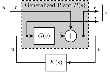
Using Matlab, the generalized plant can be defined as follows:

  P = [1 -G;
       0  1;
       1 -G]

The General Synthesis Problem Formulation

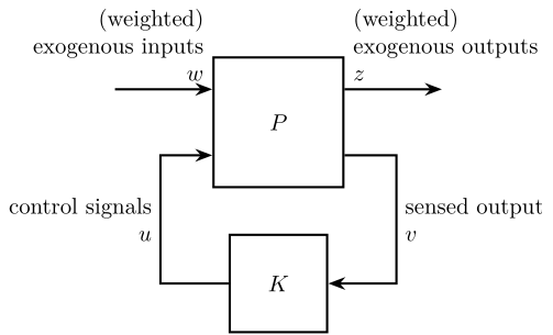
The $\mathcal{H}_\infty$ Synthesis objective is to find all stabilizing controllers $K$ which minimize

\begin{equation} \| F_l(P, K) \|_\infty = \max_{\omega} \overline{\sigma} \big( F_l(P, K)(j\omega) \big) \end{equation}

  \begin{tikzpicture}

    % Blocs
    \node[block={2.0cm}{2.0cm}] (P) {$P$};
    \node[block={1.5cm}{1.5cm}, below=0.7 of P] (K) {$K$};

    % Input and outputs coordinates
    \coordinate[] (inputw)  at ($(P.south west)!0.75!(P.north west)$);
    \coordinate[] (inputu)  at ($(P.south west)!0.25!(P.north west)$);
    \coordinate[] (outputz) at ($(P.south east)!0.75!(P.north east)$);
    \coordinate[] (outputv) at ($(P.south east)!0.25!(P.north east)$);

    % Connections and labels
    \draw[<-] (inputw) node[above left, align=right]{(weighted)\\exogenous inputs\\$w$} -- ++(-1.5, 0);
    \draw[<-] (inputu) -- ++(-0.8, 0) |- node[left, near start, align=right]{control signals\\$u$} (K.west);

    \draw[->] (outputz) node[above right, align=left]{(weighted)\\exogenous outputs\\$z$} -- ++(1.5, 0);
    \draw[->] (outputv) -- ++(0.8, 0) |- node[right, near start, align=left]{sensed output\\$v$} (K.east);
  \end{tikzpicture}

General Control Configuration

Modern Interpretation of the Control Specifications

Introduction

• Reference tracking Overshoot, Static error, Setling time

  • $S(s) = T_{r \rightarrow \epsilon}$

• Disturbances rejection

  • $G(s) S(s) = T_{d \rightarrow \epsilon}$

• Measurement noise filtering

  • $T(s) = T_{n \rightarrow \epsilon}$

• Small command amplitude

  • $K(s) S(s) = T_{r \rightarrow u}$

• Stability

  • $S(s)$, $T(s)$, $K(s)S(s)$, $G(s)S(s)$
• Robustness to plant uncertainty (stability margins)
• Controller implementation

**

Resources

yt:?listType=playlist&list=PLn8PRpmsu08qFLMfgTEzR8DxOPE7fBiin

yt:?listType=playlist&list=PLsjPUqcL7ZIFHCObUU_9xPUImZ203gB4o