lecture-h-infinity/index.org

A brief and practical introduction to $\mathcal{H}_\infty$ Control

• Introduction
• Introduction to the Control Methodology - Model Based Control
  • Model Based Control - Methodology
  • Some Background: From Classical Control to Robust Control
  • Example System
• Classical Open Loop Shaping
  • Introduction to Loop Shaping
  • Example of Open Loop Shaping
  • $\mathcal{H}_\infty$ Loop Shaping Synthesis
  • Example of the $\mathcal{H}_\infty$ Loop Shaping Synthesis
• First Steps in the $\mathcal{H}_\infty$ world
  • The $\mathcal{H}_\infty$ Norm
  • $\mathcal{H}_\infty$ Synthesis
  • The Generalized Plant
  • The General Synthesis Problem Formulation
  • From a Classical Feedback Architecture to a Generalized Plant
• Modern Interpretation of the Control Specifications
  • Introduction
  • Closed Loop Transfer Functions
  • Sensitivity Function
  • Robustness: Module Margin
  • How to Shape transfer function? Using of Weighting Functions!
  • Design of Weighting Functions
  • Sensitivity Function Shaping - Example
  • Complementary Sensitivity Function
  • Summary
• $\mathcal{H}_\infty$ Mixed-Sensitivity Synthesis
  • Problem
  • Typical Procedure
  • Step 1 - Shaping of the Sensitivity Function
  • Step 2 - Shaping of
  • General Configuration for various shaping
    • S KS
    • S T
    • S T KS
    • S T KS GS
• Conclusion
• Resources

TODO Introduction   ignore

Introduction to the Control Methodology - Model Based Control

<<sec:model_based_control>>

Model Based Control - Methodology

<<sec:model_based_control_methodology>>

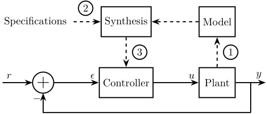
The typical methodology when applying Model Based Control to a plant is schematically shown in Figure fig:control-procedure. It consists of three steps:

1. Identification or modeling: $\Longrightarrow$ mathematical model

2. Translate the specifications into mathematical criteria:

   • Specifications: Response Time, Noise Rejection, Maximum input amplitude, Robustness, …
   • Mathematical Criteria: Cost Function, Shape of TF
3. Synthesis: research of $K$ that satisfies the specifications for the model of the system

  \begin{tikzpicture}
    \node[addb={+}{}{}{}{-}] (addsub) at (0, 0){};

    \node[block, right=1.5 of addsub] (controller) {Controller};
    \node[block, right=1.5 of controller] (plant) {Plant};

    \node[block, above=1 of controller] (controller_design) {Synthesis};
    \node[block, above=1 of plant] (model_plant) {Model};

    \draw[<-] (addsub.west) -- ++(-1, 0) node[above right]{$r$};

    \draw[->] (addsub) -- (controller.west) node[above left]{$\epsilon$};
    \draw[->] (controller) -- (plant.west) node[above left]{$u$};
    \draw[->] (plant.east) -- ++(1, 0) node[above left]{$y$};
    \draw[] ($(plant.east) + (0.5, 0)$) -- ++(0, -1);
    \draw[->] ($(plant.east) + (0.5, -1)$) -| (addsub.south);

    \draw[->, dashed] (plant) -- node[midway, right, labelc, solid]{1} (model_plant);
    \draw[->, dashed] (controller_design) --node[midway, right, labelc, solid]{3} (controller);
    \draw[->, dashed] (model_plant) -- (controller_design);
    \draw[<-, dashed] (controller_design.west) -- node[midway, above, labelc, solid]{2} ++(-1, 0) node[left, style={align=center}]{Specifications};
  \end{tikzpicture}

Typical Methodoly for Model Based Control

In this document, we will mainly focus on steps 2 and 3.

Some Background: From Classical Control to Robust Control

<<sec:comp_classical_modern_robust_control>>

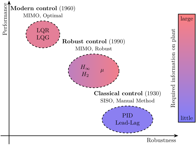
	Classical Control	Modern Control	Robust Control
Date	1930-	1960-	1980-
Tools	Transfer Functions	State Space formulation	Systems and Signals Norms ($\mathcal{H}_\infty$, $\mathcal{H}_2$ Norms)
	Nyquist Plots	Riccati Equations	Closed Loop Transfer Functions
	Bode Plots		Open/Closed Loop Shaping
	Phase and Gain margins		Weighting Functions
			Disk margin
Control Architectures	Proportional, Integral, Derivative	Full State Feedback	General Control Configuration
	Leads, Lags	LQR, LQG
		Kalman Filters
Advantages	Study Stability	Automatic Synthesis	Automatic Synthesis
	Simple	MIMO	MIMO
	Natural	Optimization Problem	Optimization Problem
			Guaranteed Robustness
			Easy specification of performances
Disadvantages	Manual Method	No Guaranteed Robustness	Required knowledge of specific tools
	Only SISO	Difficult Rejection of Perturbations	Need a reasonably good model of the system

Table summurazing the main differences between classical, modern and robust control

  \begin{tikzpicture}
    % Scale
    \def\yscale{0.8}
    \def\xscale{1.0}

    % Colors
    \def\colorstart{blue}
    \def\colorend{red}

    % Axis
    \draw [->] (-0.5,0) -- (10*\xscale,0) node[below left]{Robustness};
    \draw [->] (0,-0.5) -- (0,10*\yscale) node[below left, rotate=90, anchor=south east]{Performance};

    % Color Bar
    \shade[draw, bottom color=\colorstart, top color=\colorend, fill opacity=0.5] (10*\xscale, 1*\yscale) rectangle (11*\xscale, 9*\yscale);
    \node[rotate=90, above] at (10*\xscale, 5*\yscale) {Required information on plant};
    \node[above] at (10.5*\xscale, 1*\yscale) {little};
    \node[below] at (10.5*\xscale, 9*\yscale) {large};

    % ===================================
    % Classical Control
    % ===================================
    % Control Types
    \node[align=center] (pid)  at (7.0*\xscale, 1.2*\yscale) {PID\\Lead-Lag};

    \begin{scope}[on background layer]
      % Control Families
      \node[ellipse, draw, dashed, minimum width=3.0*\xscale cm, minimum height=2.0*\yscale cm,
          fill=\colorstart!90!\colorend, fill opacity=0.5, text opacity=1]
          (classicalcontrol) at (pid) {};
    \end{scope}
    \node[above, align=center] at (classicalcontrol.north) {\textbf{Classical control} (1930)\\{\small SISO, Manual Method}};
    % ===================================


    % ===================================
    % Modern Control
    % ===================================
    % Control Types
    \node[align=center] (lqg)  at (2.0*\xscale, 7.5*\yscale) {LQR\\LQG};

    \begin{scope}[on background layer]
      \node[ellipse, draw, dashed, minimum width=2.0*\xscale cm, minimum height=2.0*\yscale cm,
          fill=\colorstart!20!\colorend, fill opacity=0.5, text opacity=1]
          (moderncontrol) at (lqg) {};
    \end{scope}
    \node[above, align=center] at (moderncontrol.north) {\textbf{Modern control} (1960)\\{\small MIMO, Optimal}};
    % ===================================


    % ===================================
    % Robust Control
    % ===================================
    % Control Types
    \node[align=center] (hinf) at (4.5*\xscale, 4.8*\yscale) {$H_\infty$\\$H_2$};
    \node[] (mu) at (5.5*\xscale, 4.8*\yscale) {$\mu$};


    \begin{scope}[on background layer]
      \node[ellipse, draw, dashed, minimum width=3.0*\xscale cm, minimum height=2.5*\yscale cm,
          shade, left color=\colorstart!50!\colorend, right color=\colorstart!10!\colorend, fill opacity=0.5, text opacity=1]
          (robustcontrol) at ($0.5*(hinf)+0.5*(mu)$) {};
    \end{scope}
    \node[above, align=center] at (robustcontrol.north) {\textbf{Robust control} (1990)\\{\small MIMO, Robust}};
    % ===================================
  \end{tikzpicture}

Comparison of the performance and robustness of classical control methods, modern control methods and robust control methods. The required information on the plant to succesfuly apply each of the control methods are indicated by the colors.

Example System

<<sec:example_system>>

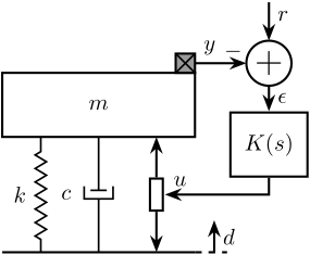
Let's consider the model shown in Figure fig:mech_sys_1dof_inertial_contr. It could represent a suspension system with a payload to position or isolate using an force actuator and an inertial sensor. The notations used are listed in Table tab:example_notations.

  \begin{tikzpicture}
    % Parameters
    \def\massw{3}
    \def\massh{1}
    \def\spaceh{1.8}

    % Ground
    \draw[] (-0.5*\massw, 0) -- (0.5*\massw, 0);
    % Mass
    \draw[fill=white] (-0.5*\massw, \spaceh) rectangle (0.5*\massw, \spaceh+\massh) node[pos=0.5](m){$m$};

    % Spring, Damper, and Actuator
    \draw[spring]   (-0.3*\massw, 0) -- (-0.3*\massw, \spaceh) node[midway, left=0.1]{$k$};
    \draw[damper]   ( 0, 0) -- ( 0, \spaceh) node[midway, left=0.3]{$c$};
    \draw[actuator] ( 0.3*\massw, 0) -- (0.3*\massw, \spaceh) node[midway](F){};

    % Displacements
    \draw[dashed] (0.5*\massw, 0) -- ++(0.5, 0);
    \draw[->] (0.6*\massw, 0) -- ++(0, 0.5) node[below right]{$d$};

    % Inertial Sensor
    \node[inertialsensor] (inertials) at (0.5*\massw, \spaceh+\massh){};
    \node[addb={+}{-}{}{}{}, right=0.8 of inertials] (subf) {};

    \node[block, below=0.4 of subf] (K){$K(s)$};

    \draw[->] (inertials.east) node[above right]{$y$} -- (subf.west);
    \draw[->] (subf.south) -- (K.north) node[above right]{$\epsilon$};
    \draw[<-] (subf.north) -- ++(0, 0.6) node[below right]{$r$};
    \draw[->] (K.south) |- (F.east) node[above right]{$u$};
  \end{tikzpicture}

Test System consisting of a payload with a mass $m$ on top of an active system with a stiffness $k$, damping $c$ and an actuator. A feedback controller $K(s)$ is added to position / isolate the payload.

Notation	Description	Value	Unit
$m$	Payload's mass to position / isolate	$10$	[kg]
$k$	Stiffness of the suspension system	$10^6$	[N/m]
$c$	Damping coefficient of the suspension system	$400$	[N/(m/s)]
$y$	Payload absolute displacement (measured by an inertial sensor)		[m]
$d$	Ground displacement, it acts as a disturbance		[m]
$u$	Actuator force		[N]
$r$	Wanted position of the mass (the reference)		[m]
$\epsilon = r - y$	Position error		[m]
$K$	Feedback controller	to be designed	[N/m]

Example system variables

Derive the following open-loop transfer functions:

\begin{align} G(s) &= \frac{y}{u} \\ G_d(s) &= \frac{y}{d} \end{align}

Hint

You can follow this generic procedure:

1. List all applied forces ot the mass: Actuator force, Stiffness force (Hooke's law), …
2. Apply the Newton's Second Law on the payload \[ m \ddot{y} = \Sigma F \]
3. Transform the differential equations into the Laplace domain: \[ \frac{d\ \cdot}{dt} \Leftrightarrow \cdot \times s \]
4. Write $y(s)$ as a function of $u(s)$ and $w(s)$

Results

\begin{align} G(s) &= \frac{1}{m s^2 + cs + k} \\ G_d(s) &= \frac{cs + k}{m s^2 + cs + k} \end{align}

Hi Musa, Thank you very much for sharing this awesome package. For a long time, I am dreaming of being abble to export source blocks to HTML tha are surounded by <details> blocks.

For now, I am manually adding #+HTML: <details><summary>Code</summary> and #+HTML: </details> around the source blocks I want to hide… This is a very simple solution, but not so elegent nor practical.

Do you have any idea if it would be easy to extend to org-mode export of source blocks to add such functionallity?

Similarly, I would love to be able to export a <span> block with the name of the file corresponding to the source block. For instance, if a particular source block is tangled to script.sh, it would be so nice to display the filename when exporting!

Thanks in advance

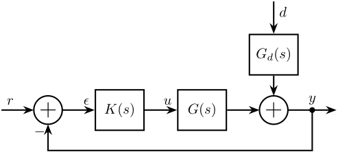
Having obtained $G(s)$ and $G_d(s)$, we can transform the system shown in Figure fig:mech_sys_1dof_inertial_contr into a classical feedback form as shown in Figure fig:open_loop_shaping.

  \begin{tikzpicture}
    \node[addb={+}{}{}{}{-}] (addfb) at (0, 0){};
    \node[block, right=0.8 of addfb] (K){$K(s)$};
    \node[block, right=0.8 of K] (G){$G(s)$};
    \node[addb={+}{}{}{}{}, right=0.8 of G] (addd){};
    \node[block, above=0.5 of addd] (Gd){$G_d(s)$};

    \draw[<-] (addfb.west) -- ++(-0.8, 0) node[above right]{$r$};
    \draw[->] (addfb.east) -- (K.west) node[above left]{$\epsilon$};
    \draw[->] (K.east) -- (G.west) node[above left]{$u$};
    \draw[->] (G.east) -- (addd.west);
    \draw[<-] (Gd.north) -- ++(0, 0.8) node[below right]{$d$};
    \draw[->] (Gd.south) -- (addd.north);
    \draw[->] (addd.east) -- ++(1.2, 0);
    \draw[->] ($(addd.east) + (0.6, 0)$) node[branch]{} node[above]{$y$} -- ++(0, -1.0) -| (addfb.south);
  \end{tikzpicture}

Block diagram corresponding to the example system

Let's define the system parameters on Matlab.

  k = 1e6; % Stiffness [N/m]
  c = 4e2; % Damping [N/(m/s)]
  m = 10; % Mass [kg]

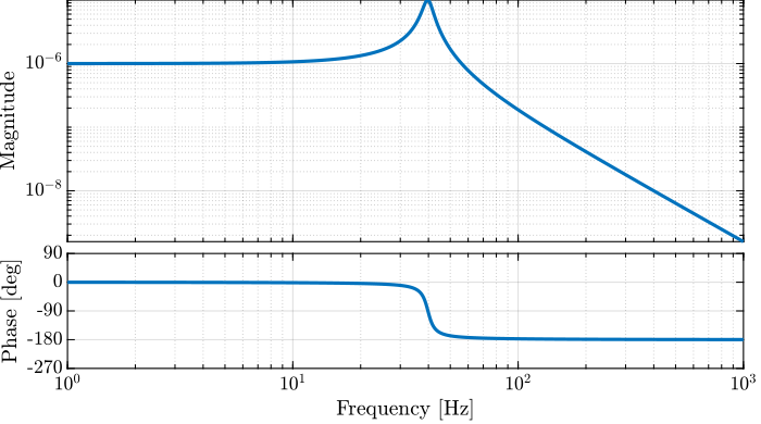
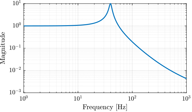
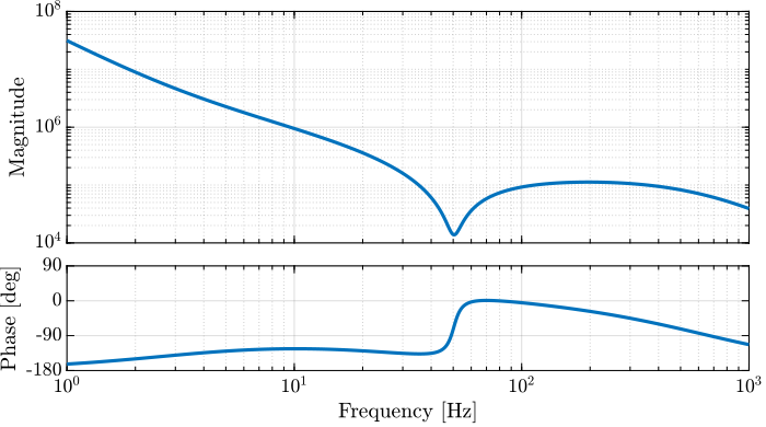
And now the system dynamics $G(s)$ and $G_d(s)$ (their bode plots are shown in Figures fig:bode_plot_example_afm and fig:bode_plot_example_Gd).

  G = 1/(m*s^2 + c*s + k); % Plant
  Gd = (c*s + k)/(m*s^2 + c*s + k); % Disturbance

Bode plot of the plant $G(s)$

Magnitude of the disturbance transfer function $G_d(s)$

Classical Open Loop Shaping

<<sec:open_loop_shaping>>

Introduction to Loop Shaping

<<sec:open_loop_shaping_introduction>>

Loop Shaping refers to a design procedure that involves explicitly shaping the magnitude of the Loop Transfer Function $L(s)$.

The Loop Gain $L(s)$ usually refers to as the product of the controller and the plant ("Gain around the loop", see Figure fig:open_loop_shaping):

\begin{equation} L(s) = G(s) \cdot K(s) \label{eq:loop_gain} \end{equation}

  \begin{tikzpicture}
    \node[addb={+}{}{}{}{-}] (addsub) at (0, 0){};

    \node[block, right=0.8 of addsub] (K) {$K(s)$};
    \node[below] at (K.south) {Controller};
    \node[block, right=0.8 of K] (G) {$G(s)$};
    \node[below] at (G.south) {Plant};

    \draw[<-] (addsub.west) -- ++(-0.8, 0) node[above right]{$r$};

    \draw[->] (addsub) -- (K.west) node[above left]{$\epsilon$};
    \draw[->] (K.east) -- (G.west) node[above left]{$u$};
    \draw[->] (G.east) -- ++(0.8, 0) node[above left]{$y$};
    \draw[] ($(G.east) + (0.5, 0)$) -- ++(0, -1.4);
    \draw[->] ($(G.east) + (0.5, -1.4)$) -| (addsub.south);

    \draw [decoration={brace, raise=5pt}, decorate] (K.north west) -- node[above=6pt]{$L(s)$} (G.north east);
  \end{tikzpicture}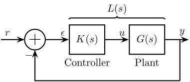

Classical Feedback Architecture

This synthesis method is widely used as many characteristics of the closed-loop system depend on the shape of the open loop gain $L(s)$ such as:

• Performance: $L$ large
• Good disturbance rejection: $L$ large
• Limitation of measurement noise on plant output: $L$ small
• Small magnitude of input signal: $K$ and $L$ small
• Nominal stability: $L$ small (RHP zeros and time delays)
• Robust stability: $L$ small (neglected dynamics)

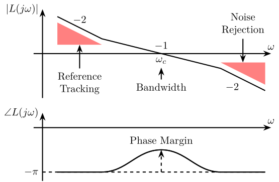
The Open Loop shape is usually done manually has the loop gain $L(s)$ depends linearly on $K(s)$ eqref:eq:loop_gain.

$K(s)$ then consists of a combination of leads, lags, notches, etc. such that $L(s)$ has the wanted shape (an example is shown in Figure fig:open_loop_shaping_shape).

  \begin{tikzpicture}
    % Phase Axis
    \draw[->] (-0.3, -0.5) -- ++(8, 0) node[above]{$\omega$}; \draw[<-] (0, 0)
    node[left]{$\angle L(j\omega)$} -- ++(0, -2.3);

    % Gain Axis
    \draw[->] (-0.3, 2) -- ++(8, 0) node[above]{$\omega$}; \draw[->] (0, 0.5) --
    ++(0, 3) node[left]{$\left|L(j\omega)\right|$};

    % Gain Slopes
    \draw[shift={(0,2)}] (0.5, 1.25) -- node[midway, above]{$-2$} (2, 0.5) --
    node[midway, above]{$-1$} (6, -0.5) -- node[midway, below left]{$-2$} (7.5,
    -1.25);

    % Forbiden region
    \path[shift={(0,1.8)}, fill=red!50!white] (0.5, 1.25) -- (2, 0.5) -| coordinate[near start](lfshaping) cycle;
    \path[shift={(0,2.2)}, fill=red!50!white] (6, -0.5) -- (7.5, -1.25) |- coordinate[near end](hfshaping) cycle;

    \draw[<-] (lfshaping) -- ++(0, -0.8) node[below, align=center]{Reference\\Tracking};
    \draw[<-] (hfshaping) -- ++(0,  0.8)  node[above, align=center]{Noise\\Rejection};

    % Crossover frequency
    \node[below] (wc) at (4,2){$\omega_c$};
    \draw[<-] (wc.south) -- ++(0, -0.4) node[below, align=center]{Bandwidth};

    % Phase
    \draw[] (0.5, -2) -- (2, -2)[out=0, in=-180] to (4, -1.25)[out=0, in=-180] to
    (6, -2) -- (7.5, -2); \draw[] (0.5, -2) -- (2, -2)[out=0, in=-180] to (4,
    -1.25)[out=0, in=-180] to (6, -2) -- (7.5, -2);

    % Phase Margin
    \draw[->, dashed] (4, -2) -- (4, -1.25) node[above]{Phase Margin};
    \draw[dashed] (0, -2) node[left]{$-\pi$} -- (7.5, -2);
  \end{tikzpicture}

Typical Wanted Shape for the Loop Gain $L(s)$

Example of Open Loop Shaping

<<sec:loop_shaping_example>>

Let's take our example system and try to apply the Open-Loop shaping strategy to design a controller that fulfils the following specifications:

• Performance: Bandwidth of approximately 10Hz
• Noise Attenuation: Roll-off of -40dB/decade past 30Hz
• Robustness: Gain margin > 3dB and Phase margin > 30 deg

Using SISOTOOL, design a controller that fulfill the specifications.

  sisotool(G)

In order to have the wanted Roll-off, two integrators are used, a lead is also added to have sufficient phase margin.

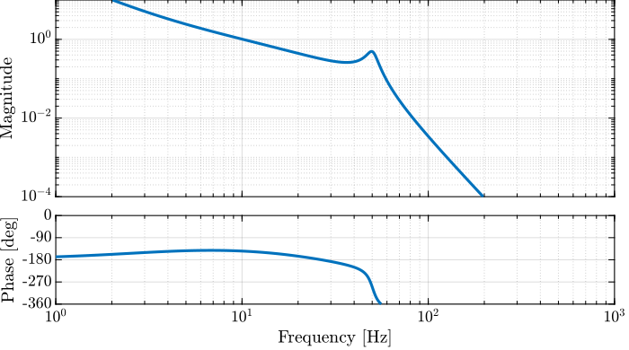
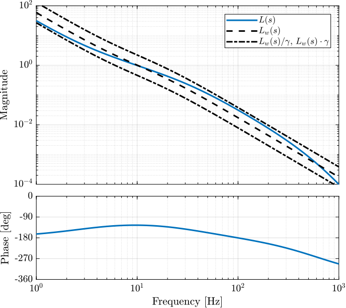
The obtained controller is shown below, and the bode plot of the Loop Gain is shown in Figure fig:loop_gain_manual_afm.

  K = 14e8 * ... % Gain
      1/(s^2) * ... % Double Integrator
      1/(1 + s/2/pi/40) * ... % Low Pass Filter
      (1 + s/(2*pi*10/sqrt(8)))/(1 + s/(2*pi*10*sqrt(8))); % Lead

Bode Plot of the obtained Loop Gain $L(s) = G(s) K(s)$

And we can verify that we have the wanted stability margins:

  [Gm, Pm, ~, Wc] = margin(G*K)

Requirements	Manual Method
Gain Margin $> 3$ [dB]	3.1
Phase Margin $> 30$ [deg]	35.4
Crossover $\approx 10$ [Hz]	10.1

$\mathcal{H}_\infty$ Loop Shaping Synthesis

<<sec:h_infinity_open_loop_shaping>>

The Open Loop Shaping synthesis can be performed using the $\mathcal{H}_\infty$ Synthesis.

Even though we will not go into details, we will provide one example.

Using Matlab, the $\mathcal{H}_\infty$ Loop Shaping Synthesis can be performed using the loopsyn command:

  K = loopsyn(G, Gd);

where:

• G is the (LTI) plant
• Gd is the wanted loop shape
• K is the synthesize controller

Matlab documentation of loopsyn (link).

Example of the $\mathcal{H}_\infty$ Loop Shaping Synthesis

<<sec:h_infinity_open_loop_shaping_example>>

Let's reuse the previous plant.

Translate the specification into the wanted shape of the open loop gain.

• Performance: Bandwidth of approximately 10Hz: $|L_w(j2 \pi 10)| = 1$
• Noise Attenuation: Roll-off of -40dB/decade past 30Hz
• Robustness: Gain margin > 3dB and Phase margin > 30 deg

  Lw = 2.3e3 * ...
       1/(s^2) * ... % Double Integrator
       (1 + s/(2*pi*10/sqrt(3)))/(1 + s/(2*pi*10*sqrt(3))); % Lead

The $\mathcal{H}_\infty$ optimal open loop shaping synthesis is performed using the loopsyn command:

  [K, ~, GAM] = loopsyn(G, Lw);

The Bode plot of the obtained controller is shown in Figure fig:open_loop_shaping_hinf_K.

It is always important to analyze the controller after the synthesis is performed.

In the end, a synthesize controller is just a combination of low pass filters, high pass filters, notches, leads, etc.

Let's briefly analyze this controller:

• two integrators are used at low frequency to have the wanted low frequency high gain
• a lead is added centered with the crossover frequency to increase the phase margin
• a notch is added at the resonance of the plant to increase the gain margin (this is very typical of $\mathcal{H}_\infty$ controllers, and can be an issue, more info on that latter)

Obtained controller $K$ using the open-loop $\mathcal{H}_\infty$ shaping

The obtained Loop Gain is shown in Figure fig:open_loop_shaping_hinf_L.

Obtained Open Loop Gain $L(s) = G(s) K(s)$ and comparison with the wanted Loop gain $L_w$

Let's now compare the obtained stability margins of the $\mathcal{H}_\infty$ controller and of the manually developed controller in Table tab:open_loop_shaping_compare.

Specifications	Manual Method	$\mathcal{H}_\infty$ Method
Gain Margin $> 3$ [dB]	3.1	31.7
Phase Margin $> 30$ [deg]	35.4	54.7
Crossover $\approx 10$ [Hz]	10.1	9.9

Comparison of the characteristics obtained with the two methods

First Steps in the $\mathcal{H}_\infty$ world

<<sec:h_infinity_introduction>>

The $\mathcal{H}_\infty$ Norm

<<sec:h_infinity_norm>>

The $\mathcal{H}_\infty$ norm is defined as the peak of the maximum singular value of the frequency response

\begin{equation} \|G(s)\|_\infty = \max_\omega \bar{\sigma}\big( G(j\omega) \big) \end{equation}

For a SISO system $G(s)$, it is simply the peak value of $|G(j\omega)|$ as a function of frequency:

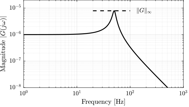
\begin{equation} \|G(s)\|_\infty = \max_{\omega} |G(j\omega)| \label{eq:hinf_norm_siso} \end{equation}

Let's compute the $\mathcal{H}_\infty$ norm of our test plant $G(s)$ using the hinfnorm function:

  hinfnorm(G)

7.9216e-06

We can see that the $\mathcal{H}_\infty$ norm of $G(s)$ does corresponds to the peak value of $|G(j\omega)|$ as a function of frequency as shown in Figure fig:hinfinity_norm_siso_bode.

Example of the $\mathcal{H}_\infty$ norm of a SISO system

$\mathcal{H}_\infty$ Synthesis

<<sec:h_infinity_synthesis>>

$\mathcal{H}_\infty$ synthesis is a method that uses an algorithm (LMI optimization, Riccati equation) to find a controller that stabilize the system and that minimizes the $\mathcal{H}_\infty$ norms of defined transfer functions.

Why optimizing the $\mathcal{H}_\infty$ norm of transfer functions is a pertinent choice will become clear when we will translate the typical control specifications into the $\mathcal{H}_\infty$ norm of transfer functions.

Then applying the $\mathcal{H}_\infty$ synthesis to a plant, the engineer work usually consists of the following steps

1. Write the problem as standard $\mathcal{H}_\infty$ problem
2. Translate the specifications as $\mathcal{H}_\infty$ norms of transfer functions
3. Make the synthesis and analyze the obtain controller
4. Reduce the order of the controller for implementation

Note that there are many ways to use the $\mathcal{H}_\infty$ Synthesis:

• Traditional $\mathcal{H}_\infty$ Synthesis (hinfsyn doc)
• Open Loop Shaping $\mathcal{H}_\infty$ Synthesis (loopsyn doc)
• Mixed Sensitivity Loop Shaping (mixsyn doc)
• Fixed-Structure $\mathcal{H}_\infty$ Synthesis (hinfstruct doc)
• Signal Based $\mathcal{H}_\infty$ Synthesis

The Generalized Plant

<<sec:generalized_plant>>

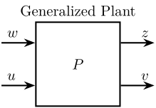
The first step when applying the $\mathcal{H}_\infty$ synthesis is usually to write the problem as a standard $\mathcal{H}_\infty$ problem. This consist of deriving the Generalized Plant for the current problem. It makes things much easier for the following steps.

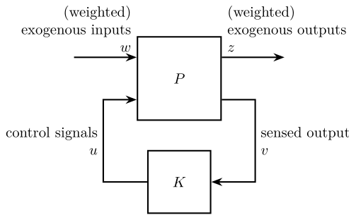
The generalized plant, usually noted $P(s)$, is shown in Figure fig:general_plant. It has two inputs and two outputs (both could contains many signals). The meaning of the inputs and outputs are summarized in Table tab:notation_general.

Note that this generalized plant is as its name implies, quite general. It can indeed represent feedback as well as feedforward control architectures.

\begin{equation} \begin{bmatrix} z \\ v \end{bmatrix} = P \begin{bmatrix} w \\ u \end{bmatrix} = \begin{bmatrix} P_{11} & P_{12} \\ P_{21} & P_{22} \end{bmatrix} \begin{bmatrix} w \\ u \end{bmatrix} \end{equation}

  \begin{tikzpicture}
    \node[block={2.0cm}{2.0cm}] (P) {$P$};
    \node[above] at (P.north) {Generalized Plant};

    % Input and outputs coordinates
    \coordinate[] (inputw)  at ($(P.south west)!0.75!(P.north west)$);
    \coordinate[] (inputu)  at ($(P.south west)!0.25!(P.north west)$);
    \coordinate[] (outputz) at ($(P.south east)!0.75!(P.north east)$);
    \coordinate[] (outputv) at ($(P.south east)!0.25!(P.north east)$);

    % Connections and labels
    \draw[<-] (inputw) -- ++(-0.8, 0) node[above right]{$w$};
    \draw[<-] (inputu) -- ++(-0.8, 0) node[above right]{$u$};

    \draw[->] (outputz) -- ++(0.8, 0) node[above left]{$z$};
    \draw[->] (outputv) -- ++(0.8, 0) node[above left]{$v$};
  \end{tikzpicture}

Inputs and Outputs of the generalized Plant

Notation	Meaning
$P$	Generalized plant model
$w$	Exogenous inputs: commands, disturbances, noise
$z$	Exogenous outputs: signals to be minimized
$v$	Controller inputs: measurements
$u$	Control signals

Notations for the general configuration

The General Synthesis Problem Formulation

<<sec:h_infinity_general_synthesis>>

Once the generalized plant is obtained, the $\mathcal{H}_\infty$ synthesis problem can be stated as follows:

$\mathcal{H}_\infty$ Synthesis applied on the generalized plant

Find a stabilizing controller $K$ that, using the sensed output $v$, generates a control signal $u$ such that the $\mathcal{H}_\infty$ norm of the closed-loop transfer function from $w$ to $z$ is minimized.

After $K$ is found, the system is robustified by adjusting the response around the unity gain frequency to increase stability margins.

  \begin{tikzpicture}

    % Blocs
    \node[block={2.0cm}{2.0cm}] (P) {$P$};
    \node[block={1.5cm}{1.5cm}, below=0.7 of P] (K) {$K$};

    % Input and outputs coordinates
    \coordinate[] (inputw)  at ($(P.south west)!0.75!(P.north west)$);
    \coordinate[] (inputu)  at ($(P.south west)!0.25!(P.north west)$);
    \coordinate[] (outputz) at ($(P.south east)!0.75!(P.north east)$);
    \coordinate[] (outputv) at ($(P.south east)!0.25!(P.north east)$);

    % Connections and labels
    \draw[<-] (inputw) node[above left, align=right]{(weighted)\\exogenous inputs\\$w$} -- ++(-1.5, 0);
    \draw[<-] (inputu) -- ++(-0.8, 0) |- node[left, near start, align=right]{control signals\\$u$} (K.west);

    \draw[->] (outputz) node[above right, align=left]{(weighted)\\exogenous outputs\\$z$} -- ++(1.5, 0);
    \draw[->] (outputv) -- ++(0.8, 0) |- node[right, near start, align=left]{sensed output\\$v$} (K.east);
  \end{tikzpicture}

General Control Configuration

Note that the closed-loop transfer function from $w$ to $z$ is:

\begin{equation} \frac{z}{w} = P_{11} + P_{12} K \big( I - P_{22} K \big)^{-1} P_{21} \triangleq F_l(P, K) \end{equation}

Using Matlab, the $\mathcal{H}_\infty$ Synthesis applied on a Generalized plant can be applied using the hinfsyn command (documentation):

  K = hinfsyn(P, nmeas, ncont);

where:

• P is the generalized plant transfer function matrix
• nmeas is the number of sensed output (size of $v$)
• ncont is the number of control signals (size of $u$)
• K obtained controller that minimized the $\mathcal{H}_\infty$ norm from $w$ to $z$

From a Classical Feedback Architecture to a Generalized Plant

<<sec:generalized_plant_derivation>>

The procedure to convert a typical control architecture as the one shown in Figure fig:classical_feedback_tracking to a generalized Plant is as follows:

1. Define signals ($w$, $z$, $u$ and $v$) of the generalized plant
2. Remove $K$ and rearrange the inputs and outputs to match the generalized configuration

  \begin{tikzpicture}
    \node[addb={+}{}{}{}{-}] (addfb) at (0, 0){};
    \node[block, right=0.8 of addfb] (K){$K(s)$};
    \node[block, right=0.8 of K] (G){$G(s)$};

    \draw[<-] (addfb.west) -- ++(-0.8, 0) node[above right]{$r$};
    \draw[->] (addfb.east) -- (K.west) node[above left]{$\epsilon$};
    \draw[->] (K.east) -- (G.west) node[above left]{$u$};
    \draw[->] (G.east) -- ++(1.2, 0);
    \draw[->] ($(G.east) + (0.6, 0)$) node[branch]{} node[above]{$y$} -- ++(0, -0.8) -| (addfb.south);
  \end{tikzpicture}

  \begin{tikzpicture}
    \node[block] (G) {$G(s)$};
    \node[addb={+}{-}{}{}{}, right=0.6 of G] (addw) {};
    \coordinate[above right=0.6 and 1.4 of addw] (u);
    \coordinate[above=0.6 of u] (epsilon);

    \coordinate[] (w) at ($(epsilon-|G.west)+(-1.4, 0)$);

    \node[block, below left=0.8 and 0 of addw] (K) {$K(s)$};

    % Connections
    \draw[->] (G.east) -- (addw.west);
    \draw[->] ($(addw.east)+(0.4, 0)$)node[branch]{} |- (epsilon) node[above left](z1){$\epsilon$};
    \draw[->] ($(G.west)+(-0.4, 0)$)node[branch](start){} |- (u) node[above left](z2){$u$};

    \draw[->] (addw.east) -- (addw-|z1) |- node[near start, right]{$v$} (K.east);
    \draw[->] (K.west) -| node[near end, left]{$u$} ($(G-|w)+(0.4, 0)$) -- (G.west);

    \draw[->] (w) node[above]{$w = r$} -| (addw.north);

    \draw [decoration={brace, raise=5pt}, decorate] (z1.north east) -- node[right=6pt]{$z$} (z2.south east);

    \begin{scope}[on background layer]
      \node[fit={(G.south-|start.west) ($(z1.north west)+(-0.4, 0)$)}, inner sep=6pt, draw, dashed, fill=black!20!white] (P) {};
      \node[below] at (P.north) {Generalized Plant $P(s)$};
    \end{scope}
  \end{tikzpicture}

Compute the Generalized plant of corresponding to the tracking control architecture shown in Figure fig:classical_feedback_tracking

Classical Feedback Control Architecture (Tracking)

Hint

First, define the signals of the generalized plant:

• Exogenous inputs: $w = r$
• Signals to be minimized: $z_1 = \epsilon$, $z_2 = u$
• Control signals: $v = y$
• Control inputs: $u$

Then, Remove $K$ and rearrange the inputs and outputs.

Answer

The obtained generalized plant shown in Figure fig:mixed_sensitivity_ref_tracking.

Generalized plant of the Classical Feedback Control Architecture (Tracking)

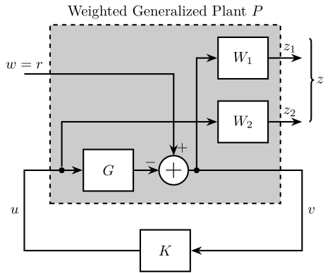
Using Matlab, the generalized plant can be defined as follows:

  P = [1 -G;
       0  1;
       1 -G]
  P.InputName = {'w', 'u'};
  P.OutputName = {'e', 'u', 'v'};

Modern Interpretation of the Control Specifications

<<sec:modern_interpretation_specification>>

Introduction

As shown in Section sec:open_loop_shaping, the loop gain $L(s) = G(s) K(s)$ is a useful and easy tool for the design of controllers by hand.

It is very easy to shape as it depends linearly on $K(s)$. Moreover, it gives information on important quantities such as the stability margins and the control bandwidth.

However, the loop gain $L(s)$ does not directly give the performances of the closed-loop system. The closed loop system behavior is determined by the closed-loop transfer functions.

If we consider the feedback system shown in Figure fig:gang_of_four_feedback, we can link to the following specifications to closed-loop transfer functions

• Reference tracking (Overshoot, Static error, Settling time, …)

  • From $r$ to $\epsilon$

• Disturbances rejection

  • From $d$ to $y$

• Measurement noise filtering

  • From $n$ to $y$

• Small command amplitude

  • From $n, r, d$ to $u$

• Stability

  • All closed-loop transfer functions must be stable

• Robustness (stability margins)

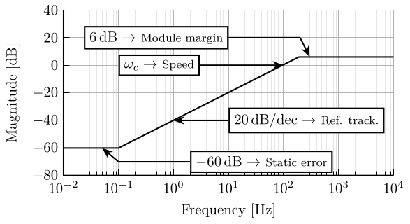
  • Module margin (see Section sec:module_margin)

  \begin{tikzpicture}
    \node[addb={+}{}{}{}{-}] (addfb) at (0, 0){};
    \node[block, right=0.8 of addfb] (K){$K(s)$};
    \node[addb,  right=0.8 of K] (addd){};
    \node[block, right=0.8 of addd] (G){$G(s)$};
    \node[addb,  below right=0.4 and 0.2 of G] (addn){};

    \draw[<-] (addfb.west) -- ++(-0.8, 0) node[above right]{$r$};
    \draw[->] (addfb.east) -- (K.west) node[above left]{$\epsilon$};
    \draw[->] (K.east) -- (addd.west);
    \draw[<-] (addd.north) -- ++(0, 0.6) node[below right]{$d$};
    \draw[->] (addd.east) -- (G.west) node[above left]{$u$};
    \draw[->] (G.east) -- ++(1.6, 0) node[above left]{$y$};
    \draw[->] (G-|addn) node[branch]{} -- (addn.north);
    \draw[<-] (addn.east) -- ++(0.8, 0) node[above left]{$n$};
    \draw[->] (addn.west) -| (addfb.south);
  \end{tikzpicture}

Simple Feedback Architecture

Closed Loop Transfer Functions

<<sec:closed_loop_tf>>

As the performances of a controlled system depend on the closed loop transfer functions, it is very important to derive these closed-loop transfer functions as a function of the plant $G(s)$ and controller $K(s)$.

Write the output signals $[\epsilon, u, y]$ as a function of the systems $K(s), G(s)$ and of the input signals $[r, d, n]$ as shown in Figure fig:gang_of_four_feedback.

Hint

Take one of the output (e.g. $y$), and write it as a function of the inputs $[d, r, n]$ going step by step around the loop:

\begin{aligned} y &= G u \\ &= G (d + K \epsilon) \\ &= G \big(d + K (r - n - y) \big) \\ &= G d + GK r - GK n - GK y \end{aligned}

Isolate $y$ at the right hand side, and finally obtain: \[ y = \frac{GK}{1+ GK} r + \frac{G}{1 + GK} d - \frac{GK}{1 + GK} n \]

Do the same procedure for $u$ and $\epsilon$

Anwser

The following equations should be obtained:

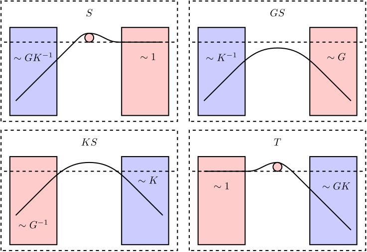
\begin{align} y &= \frac{GK}{1 + GK} r + \frac{G}{1 + GK} d - \frac{GK}{1 + GK} n \\ \epsilon &= \frac{1 }{1 + GK} r - \frac{G}{1 + GK} d - \frac{G }{1 + GK} n \\ u &= \frac{K }{1 + GK} r - \frac{1}{1 + GK} d - \frac{K }{1 + GK} n \end{align}

We can see that they are 4 different transfer functions describing the behavior of the system in Figure fig:gang_of_four_feedback. These called the Gang of Four:

\begin{align} S &= \frac{1 }{1 + GK}, \quad \text{the sensitivity function} \\ T &= \frac{GK}{1 + GK}, \quad \text{the complementary sensitivity function} \\ GS &= \frac{G }{1 + GK}, \quad \text{the load disturbance sensitivity function} \\ KS &= \frac{K }{1 + GK}, \quad \text{the noise sensitivity function} \end{align}

If a feedforward controller is included, a Gang of Six transfer functions can be defined. More on that in this short video.

And we have:

\begin{align} \epsilon &= S r - GS d - GS n \\ y &= T r + GS d - T n \\ u &= KS r - S d - KS n \end{align}

Thus, for reference tracking, we want to shape the closed-loop transfer function from $r$ to $\epsilon$, that is the sensitivity function $S(s)$. Similarly, to reduce the effect of measurement noise $n$ on the output $y$, we want to act on the complementary sensitivity function $T(s)$.

Sensitivity Function

<<sec:sensitivity_transfer_functions>>

  K1 = 14e8 * ... % Gain
       1/(s^2) * ... % Double Integrator
       (1 + s/(2*pi*10/sqrt(8)))/(1 + s/(2*pi*10*sqrt(8))); % Lead

  K2 = 1e8 * ... % Gain
       1/(s^2) * ... % Double Integrator
       (1 + s/(2*pi*1/sqrt(8)))/(1 + s/(2*pi*1*sqrt(8))); % Lead

  K3 = 1e8 * ... % Gain
       1/(s^2) * ... % Double Integrator
       (1 + s/(2*pi*1/sqrt(2)))/(1 + s/(2*pi*1*sqrt(2))); % Lead

  S1 = 1/(1 + K1*G);
  S2 = 1/(1 + K2*G);
  S3 = 1/(1 + K3*G);

  T1 = K1*G/(1 + K1*G);
  T2 = K2*G/(1 + K2*G);
  T3 = K3*G/(1 + K3*G);

  bodeFig({S1, S2, S3})

  freqs = logspace(-1, 2, 1000);

  figure;
  tiledlayout(1, 2, 'TileSpacing', 'None', 'Padding', 'None');

  ax1 = nexttile;
  hold on;
  plot(freqs, abs(squeeze(freqresp(S1, freqs, 'Hz'))), 'DisplayName', '$L(s)$');
  plot(freqs, abs(squeeze(freqresp(S2, freqs, 'Hz'))), 'DisplayName', '$L_w(s)$');
  plot(freqs, abs(squeeze(freqresp(S3, freqs, 'Hz'))), 'DisplayName', '$L_w(s) / \gamma$, $L_w(s) \cdot \gamma$');
  hold off;
  set(gca, 'XScale', 'log'); set(gca, 'YScale', 'log');
  xlabel('Frquency [Hz]'); ylabel('Sensitivity Magnitude');
  hold off;

  ax2 = nexttile;
  t = linspace(0, 1, 1000);
  y1 = step(T1, t);
  y2 = step(T2, t);
  y3 = step(T3, t);
  hold on;
  plot(t, y1)
  plot(t, y2)
  plot(t, y3)
  hold off
  xlabel('Time [s]'); ylabel('Step Response');

  \begin{tikzpicture}
    \begin{axis}[%
      width=8cm,
      height=4cm,
      at={(0,0)},
      xmode=log,
      xmin=0.01,
      xmax=10000,
      ymin=-80,
      ymax=40,
      ylabel={Magnitude [dB]},
      xlabel={Frequency [Hz]},
      ytick={40, 20, 0, -20, -40, -60, -80},
      xminorgrids,
      yminorgrids
      ]
      \addplot [thick, color=black, forget plot]
      table[row sep=crcr]{%
        0.01 -60\\
        0.1  -60\\
        190   6\\
        10000 6\\
      };
      \draw[<-] (0.05, -60) -- (0.1, -70);
      \draw (0.1, -70) -- (2, -70) node[right, fill=white, draw]{$\SI{-60}{\decibel} \rightarrow$ \footnotesize{Static error}};
      \draw[<-] (1, -40) -- (10, -40) node[right, fill=white, draw]{$\SI{20}{\decibel/dec} \rightarrow$ \footnotesize{Ref. track.}};
      \draw[<-] (100, 0) -- (3, 0) node[left, fill=white, draw]{$\omega_c \rightarrow$ \footnotesize{Speed}};

      \draw[<-] (300, 6) -- (200, 20);
      \draw (200, 20) -- (10, 20) node[left, fill=white, draw]{$\SI{6}{\decibel} \rightarrow$ \footnotesize{Module margin}};
    \end{axis}
  \end{tikzpicture}

Typical wanted shape of the Sensitivity transfer function

Robustness: Module Margin

<<sec:module_margin>>

• Definition of Module margin
• Why it represents robustness
• Example

\[ M_S < 2 \Rightarrow \text{GM} > 2 \text{ and } \text{PM} > 29^o \]

How to Shape transfer function? Using of Weighting Functions!

<<sec:weighting_functions>>

• Maybe put this section in Previous chapter

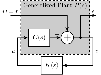
Let's say we want to shape the sensitivity transfer function corresponding to the transfer function from $r$ to $\epsilon$ of the control architecture shown in Figure fig:loop_shaping_S_without_W.

  \begin{tikzpicture}
    \node[block] (G) {$G(s)$};
    \node[addb={+}{-}{}{}{}, right=0.6 of G] (addw) {};
    \coordinate[above right=1.0 and 1.4 of addw] (epsilon);

    \coordinate[] (w) at ($(epsilon-|G.west)+(-1.0, 0)$);

    \node[block, below left=0.8 and 0 of addw] (K) {$K(s)$};

    % Connections
    \draw[->] (G.east) -- (addw.west);
    \draw[->] ($(addw.east)+(0.4, 0)$)node[branch]{} |- (epsilon) node[above left](z1){$\epsilon$};

    \draw[->] (addw.east) -- (addw-|z1) |- node[near start, right]{$v$} (K.east);
    \draw[->] (K.west) -| node[near end, left]{$u$} ($(G-|w)+(0.4, 0)$) -- (G.west);

    \draw[->] (w) node[above]{$w = r$} -| (addw.north);

    \begin{scope}[on background layer]
      \node[fit={(G.south west) ($(z1.north west)+(-0.4, 0)$)}, inner sep=12pt, draw, dashed, fill=black!20!white] (P) {};
      \node[below] at (P.north) {Generalized Plant $P(s)$};
    \end{scope}
  \end{tikzpicture}

Generalized Plant

If the $\mathcal{H}_\infty$ synthesis is directly applied on the generalized plant $P(s)$ shown in Figure fig:loop_shaping_S_without_W, if will minimize the $\mathcal{H}_\infty$ norm of transfer function from $r$ to $\epsilon$ (the sensitivity transfer function).

However, as the $\mathcal{H}_\infty$ norm is the maximum peak value of the transfer function's magnitude, it does not allow to shape the norm over all frequencies.

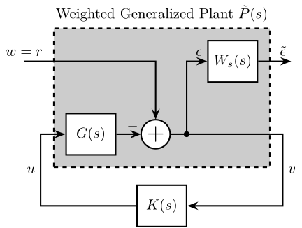
A trick is to include a weighting function in the generalized plant as shown in Figure fig:loop_shaping_S_with_W. Applying the $\mathcal{H}_\infty$ synthesis to the weighted generalized plant $\tilde{P}(s)$ (Figure fig:loop_shaping_S_with_W) will generate a controller $K(s)$ that minimizes the $\mathcal{H}_\infty$ norm between $r$ and $\tilde{\epsilon}$:

\begin{align} & \left\| \frac{\tilde{\epsilon}}{r} \right\|_\infty < \gamma (=1)\nonumber \\ \Leftrightarrow & \left\| W_s(s) S(s) \right\|_\infty < 1\nonumber \\ \Leftrightarrow & \left| W_s(j\omega) S(j\omega) \right| < 1 \quad \forall \omega\nonumber \\ \Leftrightarrow & \left| S(j\omega) \right| < \frac{1}{\left| W_s(j\omega) \right|} \quad \forall \omega \label{eq:sensitivity_shaping} \end{align}

As shown in Equation eqref:eq:sensitivity_shaping, the $\mathcal{H}_\infty$ synthesis allows to shape the magnitude of the sensitivity transfer function. Therefore, the choice of the weighting function $W_s(s)$ is very important. Its inverse magnitude will define the frequency dependent upper bound of the sensitivity transfer function magnitude.

  \begin{tikzpicture}
    \node[block] (G) {$G(s)$};
    \node[addb={+}{-}{}{}{}, right=0.6 of G] (addw) {};
    \node[block, above right=1.0 and 1.0 of addw] (Ws) {$W_s(s)$};
    \coordinate[right=0.8 of Ws] (epsilon);

    \coordinate[] (w) at ($(epsilon-|G.west)+(-1.0, 0)$);

    \begin{scope}[on background layer]
      \node[fit={(G.south west) (Ws.north east)}, inner sep=8pt, draw, dashed, fill=black!20!white] (P) {};
      \node[above] at (P.north) {Weighted Generalized Plant $\tilde{P}(s)$};
    \end{scope}

    \node[block, below=0.4 of P] (K) {$K(s)$};

    % Connections
    \draw[->] (G.east) -- (addw.west);
    \draw[->] ($(addw.east)+(0.4, 0)$)node[branch]{} |- (Ws.west)node[above left]{$\epsilon$};
    \draw[->] (Ws.east) -- (epsilon) node[above left](z1){$\tilde{\epsilon}$};

    \draw[->] (addw.east) -- (addw-|z1) |- node[near start, right]{$v$} (K.east);
    \draw[->] (K.west) -| node[near end, left]{$u$} ($(G-|w)+(0.4, 0)$) -- (G.west);

    \draw[->] (w) node[above]{$w = r$} -| (addw.north);
  \end{tikzpicture}

Weighted Generalized Plant

Once the weighting function is designed, it should be added to the generalized plant as shown in Figure fig:loop_shaping_S_with_W.

The weighted generalized plant can be defined in Matlab by either re-defining all the inputs or by pre-multiplying the (non-weighted) generalized plant by a block-diagonal MIMO transfer function containing the weights for the outputs $z$ and 1 for the outputs $v$.

  Pw = [Ws -Ws*G;
        1  -G]

  % Alternative
  Pw = blkdiag(Ws, 1)*P;

Design of Weighting Functions

<<sec:weighting_functions_design>>

Weighting function used must be proper, stable and minimum phase transfer functions.

proper

more poles than zeros, this implies $\lim_{\omega \to \infty} |W(j\omega)| < \infty$

stable

no poles in the right half plane

minimum phase

no zeros in the right half plane

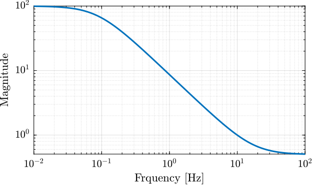
Matlab is providing the makeweight function that creates a first-order weights by specifying the low frequency gain, high frequency gain, and a gain at a specific frequency:

  W = makeweight(dcgain,[freq,mag],hfgain)

with:

• dcgain
• freq
• mag
• hfgain

The Matlab code below produces a weighting function with a magnitude shape shown in Figure fig:first_order_weight.

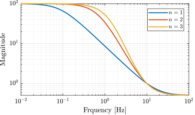
  Ws = makeweight(1e2, [2*pi*10, 1], 1/2);

Obtained Magnitude of the Weighting Function

Quite often, higher orders weights are required.

In such case, the following formula can be used the design of these weights:

\begin{equation} W(s) = \left( \frac{ \frac{1}{\omega_0} \sqrt{\frac{1 - \left(\frac{G_0}{G_c}\right)^{\frac{2}{n}}}{1 - \left(\frac{G_c}{G_\infty}\right)^{\frac{2}{n}}}} s + \left(\frac{G_0}{G_c}\right)^{\frac{1}{n}} }{ \left(\frac{1}{G_\infty}\right)^{\frac{1}{n}} \frac{1}{\omega_0} \sqrt{\frac{1 - \left(\frac{G_0}{G_c}\right)^{\frac{2}{n}}}{1 - \left(\frac{G_c}{G_\infty}\right)^{\frac{2}{n}}}} s + \left(\frac{1}{G_c}\right)^{\frac{1}{n}} }\right)^n \label{eq:weight_formula_advanced} \end{equation}

The parameters permit to specify:

• the low frequency gain: $G_0 = lim_{\omega \to 0} |W(j\omega)|$
• the high frequency gain: $G_\infty = lim_{\omega \to \infty} |W(j\omega)|$
• the absolute gain at $\omega_0$: $G_c = |W(j\omega_0)|$
• the absolute slope between high and low frequency: $n$

A Matlab function implementing Equation eqref:eq:weight_formula_advanced is shown below:

  function [W] = generateWeight(args)
      arguments
          args.G0 (1,1) double {mustBeNumeric, mustBePositive} = 0.1
          args.G1 (1,1) double {mustBeNumeric, mustBePositive} = 10
          args.Gc (1,1) double {mustBeNumeric, mustBePositive} = 1
          args.wc (1,1) double {mustBeNumeric, mustBePositive} = 2*pi
          args.n  (1,1) double {mustBeInteger, mustBePositive} = 1
      end

      if (args.Gc <= args.G0 && args.Gc <= args.G1) || (args.Gc >= args.G0 && args.Gc >= args.G1)
          eid = 'value:range';
          msg = 'Gc must be between G0 and G1';
          throwAsCaller(MException(eid,msg))
      end

      s = zpk('s');

      W = (((1/args.wc)*sqrt((1-(args.G0/args.Gc)^(2/args.n))/(1-(args.Gc/args.G1)^(2/args.n)))*s + (args.G0/args.Gc)^(1/args.n))/((1/args.G1)^(1/args.n)*(1/args.wc)*sqrt((1-(args.G0/args.Gc)^(2/args.n))/(1-(args.Gc/args.G1)^(2/args.n)))*s + (1/args.Gc)^(1/args.n)))^args.n;

  end

Matlab Function that can be used to generate Weighting functions

Let's use this function to generate three weights with the same high and low frequency gains, but but different slopes.

  W1 = generateWeight('G0', 1e2, 'G1', 1/2, 'Gc', 1, 'wc', 2*pi*10, 'n', 1);
  W2 = generateWeight('G0', 1e2, 'G1', 1/2, 'Gc', 1, 'wc', 2*pi*10, 'n', 2);
  W3 = generateWeight('G0', 1e2, 'G1', 1/2, 'Gc', 1, 'wc', 2*pi*10, 'n', 3);

The obtained shapes are shown in Figure fig:high_order_weight.

Higher order weights using Equation eqref:eq:weight_formula_advanced

Sensitivity Function Shaping - Example

<<sec:sensitivity_shaping_example>>

• Robustness: Module margin > 2 ($\Rightarrow \text{GM} > 2 \text{ and } \text{PM} > 29^o$)
• Bandwidth:
• Slope of -2

First, the weighting functions is generated.

  Ws = generateWeight('G0', 1e3, 'G1', 1/2, 'Gc', 1, 'wc', 2*pi*10, 'n', 2);

It is then added to the generalized plant.

  Pw = blkdiag(Ws, 1)*P;

And the $\mathcal{H}_\infty$ synthesis is performed.

  K = hinfsyn(Pw, 1, 1, 'Display', 'on');

K = hinfsyn(Pw, 1, 1, 'Display', 'on');

  Test bounds:  0.5 <=  gamma  <=  0.51

   gamma        X>=0        Y>=0       rho(XY)<1    p/f
  5.05e-01     0.0e+00     0.0e+00     4.497e-28     p
  Limiting gains...
  5.05e-01     0.0e+00     0.0e+00     0.000e+00     p
  5.05e-01    -1.8e+01 #  -2.9e-15     1.514e-15     f

  Best performance (actual): 0.504

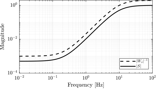
The obtained $\gamma \approx 0.5$ means that it found a controller $K(s)$ that stabilize the closed-loop system, and such that:

\begin{aligned} & \| W_s(s) S(s) \|_\infty < 0.5 \\ & \Leftrightarrow |S(j\omega)| < \frac{0.5}{|W_s(j\omega)|} \quad \forall \omega \end{aligned}

This is indeed what we can see by comparing $|S|$ and $|W_S|$ in Figure fig:results_sensitivity_hinf.

Weighting function and obtained closed-loop sensitivity

Complementary Sensitivity Function

Summary

	Open-Loop Shaping	Closed-Loop Shaping
Reference Tracking	$L$ large	$S$ small
Disturbance Rejection	$L$ large	$GS$ small
Measurement Noise Filtering	$L$ small	$T$ small
Small Command Amplitude	$K$ and $L$ small	$KS$ small
Robustness	Phase/Gain margins	Module margin: $\Vert S\Vert_\infty$ small

Table caption

  \begin{tikzpicture}
    \begin{scope}[shift={(0, 0)}]
      \draw[] (2.5, 1.0) node[]{$S$};
      \draw[fill=blue!20] (-0.2, -2.5) rectangle (1.4, 0.5);
      \draw[] (0.6, -0.5) node[]{$\sim GK^{-1}$};
      \draw[fill=red!20] (3.6, -2.5) rectangle (5.2, 0.5);
      \draw[] (4.5, -0.5) node[]{$\sim 1$};
      \draw[fill=red!20] (2.5, 0.15) circle (0.15);
      \draw[dashed] (-0.4, 0) -- (5.4, 0);
      \draw [] (0,-2) to[out=45,in=180+45] (2,0) to[out=45,in=180] (2.5,0.3) to[out=0,in=180] (3.5,0) to[out=0,in=180] (5, 0);
      \draw[dashed] (-0.5, -2.7) rectangle (5.5, 1.4);
    \end{scope}

    \begin{scope}[shift={(6.4, 0)}]
      \draw[] (2.5, 1.0) node[]{$GS$};
      \draw[fill=blue!20] (-0.2, -2.5) rectangle (1.4, 0.5);
      \draw[] (0.6, -0.5) node[]{$\sim K^{-1}$};
      \draw[fill=red!20] (3.6, -2.5) rectangle (5.2, 0.5);
      \draw[] (4.5, -0.5) node[]{$\sim G$};
      \draw[dashed] (-0.4, 0) -- (5.4, 0);
      \draw [] (0,-2) to[out=45,in=180+45] (1, -1) to[out=45, in=180] (2.5,-0.2) to[out=0,in=180-45] (4,-1) to[out=-45,in=180-45] (5, -2);
      \draw[dashed] (-0.5, -2.7) rectangle (5.5, 1.4);
    \end{scope}

    \begin{scope}[shift={(0, -4.4)}]
      \draw[] (2.5, 1.0) node[]{$KS$};
      \draw[fill=red!20] (-0.2, -2.5) rectangle (1.4, 0.5);
      \draw[] (0.6, -1.8) node[]{$\sim G^{-1}$};
      \draw[fill=blue!20] (3.6, -2.5) rectangle (5.2, 0.5);
      \draw[] (4.5, -0.3) node[]{$\sim K$};
      \draw[dashed] (-0.4, 0) -- (5.4, 0);
      \draw [] (0,-1.5) to[out=45,in=180+45] (1, -0.5) to[out=45, in=180] (2.5,0.3) to[out=0,in=180-45] (4,-0.5) to[out=-45,in=180-45] (5, -1.5);
      \draw[dashed] (-0.5, -2.7) rectangle (5.5, 1.4);
    \end{scope}

    \begin{scope}[shift={(6.4, -4.4)}]
      \draw[] (2.5, 1.0) node[]{$T$};
      \draw[fill=red!20] (-0.2, -2.5) rectangle (1.4, 0.5);
      \draw[] (0.6, -0.5) node[]{$\sim 1$};
      \draw[fill=blue!20] (3.6, -2.5) rectangle (5.2, 0.5);
      \draw[] (4.5, -0.5) node[]{$\sim GK$};
      \draw[fill=red!20] (2.5, 0.15) circle (0.15);
      \draw[dashed] (-0.4, 0) -- (5.4, 0);
      \draw [] (0,0) to[out=0,in=180] (1.5,0) to[out=0,in=180] (2.5,0.3) to[out=0,in=-45] (3,0) to[out=-45,in=180-45] (5, -2);
      \draw[dashed] (-0.5, -2.7) rectangle (5.5, 1.4);
    \end{scope}
  \end{tikzpicture}

Shaping the Gang of Four: Limitations

$\mathcal{H}_\infty$ Mixed-Sensitivity Synthesis

<<sec:h_infinity_mixed_sensitivity>>

Problem

Typical Procedure

Step 1 - Shaping of the Sensitivity Function

Step 2 - Shaping of

General Configuration for various shaping

S KS   ignore

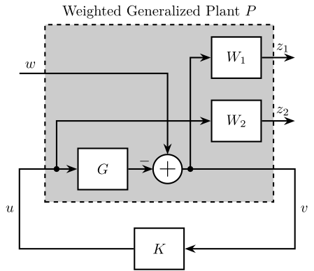
Shaping of S and KS

  \begin{tikzpicture}
    % Blocs
    \node[block] (G) {$G$};

    \node[addb={+}{-}{}{}{}, right=0.6 of G] (addw) {};
    \node[block, above right=0.4 and 0.8 of addw] (W2) {$W_2$};
    \node[block, above=0.5 of W2] (W1) {$W_1$};

    \coordinate (Gin) at ($(G.west)+(-0.5, 0)$);

    \begin{scope}[on background layer]
      \node[fit={(Gin|-G.south) (W1.north east)}, inner sep=8pt, draw, dashed, fill=black!20!white] (P) {};
      \node[above] at (P.north) {Weighted Generalized Plant $P$};
    \end{scope}

    \node[block, below=0.6 of P] (K) {$K$};

    \coordinate[right=0.8 of W1] (z);
    \coordinate[above left=1.8 and 1.4 of G] (w);

    % Connections
    \draw[->] (G.east) -- (addw.west);
    \draw[->] ($(addw.east)+(0.2, 0)$)node[branch]{} |- (W1.west);
    \draw[->] (Gin)node[branch]{} |- (W2.west);

    \draw[->] (W1.east) -- (W1-|z) node[above left](z1){$z_1$};
    \draw[->] (W2.east) -- (W2-|z) node[above left](z2){$z_2$};

    \draw[->] (addw.east) -- (addw-|z) |- node[near start, right]{$v$} (K.east);
    \draw[->] (K.west) -| node[near end, left]{$u$} (G-|w) -- (G.west);

    \draw[->] (w) node[above right]{$w$} -| (addw.north);
  \end{tikzpicture}

Generalized Plant to shape $S$ and $KS$

  P = [W1 -G*W1
       0   W2
       1  -G];

General Plant definition corresponding to Figure fig:general_conf_shaping_S_KS

• $W_1(s)$ is used to shape $S$
• $W_2(s)$ is used to shape $KS$

S T   ignore

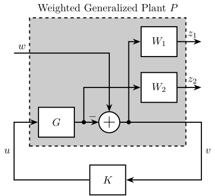
Shaping of S and T

  \begin{tikzpicture}
    % Blocs
    \node[block] (G) {$G$};

    \node[addb={+}{-}{}{}{}, right=0.8 of G] (addw) {};
    \node[block, above right=0.4 and 0.8 of addw] (W2) {$W_2$};
    \node[block, above=0.5 of W2] (W1) {$W_1$};

    \begin{scope}[on background layer]
      \node[fit={(G.south west) (W1.north east)}, inner sep=8pt, draw, dashed, fill=black!20!white] (P) {};
      \node[above] at (P.north) {Weighted Generalized Plant $P$};
    \end{scope}

    \node[block, below=0.6 of P] (K) {$K$};

    \coordinate[right=0.8 of W1] (z);
    \coordinate[above left=1.8 and 0.8 of G] (w);

    % Connections
    \draw[->] (G.east) -- (addw.west);
    \draw[->] ($(addw.east)+(0.3, 0)$)node[branch]{} |- (W1.west);
    \draw[->] ($(G.east)+(0.3, 0)$)node[branch]{} |- (W2.west);

    \draw[->] (W1.east) -- (W1-|z) node[above left](z1){$z_1$};
    \draw[->] (W2.east) -- (W2-|z) node[above left](z2){$z_2$};

    \draw[->] (addw.east) -- (addw-|z) |- node[near start, right]{$v$} (K.east);
    \draw[->] (K.west) -| node[near end, left]{$u$} (G-|w) -- (G.west);

    \draw[->] (w) node[above right]{$w$} -| (addw.north);
  \end{tikzpicture}

Generalized Plant to shape $S$ and $T$

  P = [W1 -G*W1
       0   G*W2
       1   -G];

General Plant definition corresponding to Figure fig:general_conf_shaping_S_T

• $W_1$ is used to shape $S$
• $W_2$ is used to shape $T$

S T KS   ignore

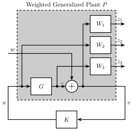
Shaping of S, T and KS

  \begin{tikzpicture}
    % Blocs
    \node[block] (G) {$G$};

    \node[addb={+}{-}{}{}{}, right=0.8 of G] (addw) {};
    \node[block, above right=0.4 and 0.8 of addw] (W3) {$W_3$};
    \node[block, above=0.2 of W3] (W2) {$W_2$};
    \node[block, above=0.2 of W2] (W1) {$W_1$};

    \coordinate (Gin) at ($(G.west)+(-0.5, 0)$);

    \begin{scope}[on background layer]
      \node[fit={(Gin|-G.south) (W1.north east)}, inner sep=8pt, draw, dashed, fill=black!20!white] (P) {};
      \node[above] at (P.north) {Weighted Generalized Plant $P$};
    \end{scope}

    \node[block, below=0.6 of P] (K) {$K$};

    \coordinate[right=0.8 of W1] (z);
    \coordinate[above left=1.4 and 1.3 of G] (w);

    % Connections
    \draw[->] (G.east) -- (addw.west);
    \draw[->] ($(addw.east)+(0.3, 0)$)node[branch]{} |- (W1.west);
    \draw[->] (Gin)node[branch]{} |- (W2.west);
    \draw[->] ($(G.east)+(0.3, 0)$)node[branch]{} |- (W3.west);

    \draw[->] (W1.east) -- (W1-|z) node[above left](z1){$z_1$};
    \draw[->] (W2.east) -- (W2-|z) node[above left](z2){$z_2$};
    \draw[->] (W3.east) -- (W3-|z) node[above left](z3){$z_3$};

    \draw[->] (addw.east) -- (addw-|z) |- node[near start, right]{$v$} (K.east);
    \draw[->] (K.west) -| node[near end, left]{$u$} (G-|w) -- (G.west);

    \draw[->] (w) node[above right]{$w$} -| (addw.north);
  \end{tikzpicture}

Generalized Plant to shape $S$, $T$ and $KS$

  P = [W1 -G*W1
       0   W2
       0   G*W3
       1   -G];

General Plant definition corresponding to Figure fig:general_conf_shaping_S_T_KS

• $W_1$ is used to shape $S$
• $W_2$ is used to shape $KS$
• $W_3$ is used to shape $T$

S T KS GS   ignore

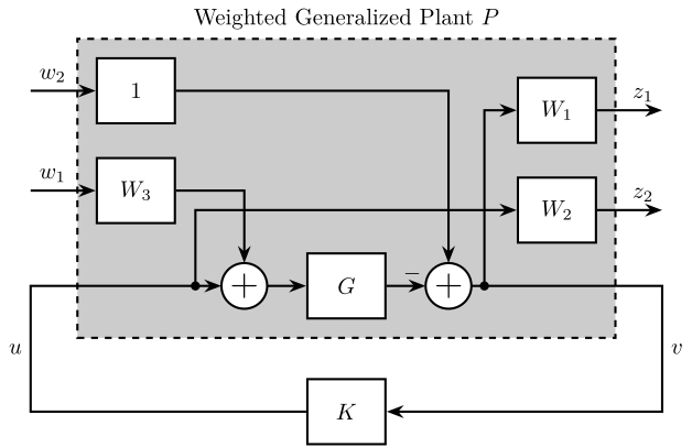
Shaping of S, T, KS and GS

  \begin{tikzpicture}
    % Blocs
    \node[block] (G) {$G$};

    \node[addb={+}{-}{}{}{}, right=0.6 of G] (addr) {};
    \node[addb, left=0.6 of G] (addd) {};
    \node[block, above right=0.4 and 0.8 of addr] (W2) {$W_2$};
    \node[block, above=0.5 of W2] (W1) {$W_1$};

    \node[block, above left=0.7 and 0.8 of addd] (W3) {$W_3$};
    \node[block, above=0.5 of W3] (W4) {$1$};

    \begin{scope}[on background layer]
      \node[fit={(W3.west|-G.south) (W4.north -| W2.east)}, inner sep=8pt, draw, dashed, fill=black!20!white] (P) {};
      \node[above] at (P.north) {Weighted Generalized Plant $P$};
    \end{scope}

    \node[block, below=0.6 of P] (K) {$K$};

    \coordinate[right=1.0 of W1] (z);
    \coordinate[left=1.0 of W3] (w);

    % Connections
    \draw[->] (G.east) -- (addr.west);
    \draw[->] ($(addr.east)+( 0.2, 0)$)node[branch]{} |- (W1.west);
    \draw[->] ($(addd.west)+(-0.4, 0)$)node[branch]{} |- (W2.west);

    \draw[->] (W1.east) -- (W1-|z) node[above left](z1){$z_1$};
    \draw[->] (W2.east) -- (W2-|z) node[above left](z2){$z_2$};

    \draw[->] (addr.east) -- (addw-|z) |- node[near start, right]{$v$} (K.east);
    \draw[->] (K.west) -| node[near end, left]{$u$} (addd-|w) -- (addd.west);
    \draw[->] (addd.east) -- (G.west);

    \draw[->] (W3.east) -| (addd.north);
    \draw[->] (W4.east) -| (addr.north);

    \draw[->] (w) node[above right]{$w_1$} -- (W3.west);
    \draw[->] (w|-W4) node[above right]{$w_2$} -- (W4.west);
  \end{tikzpicture}

Generalized Plant to shape $S$, $T$, $KS$ and $GS$

  P = [ W1  -W1*G*W3 -G*W1
        0    0        W2
        1   -G*W3    -G];

General Plant definition corresponding to Figure fig:general_conf_shaping_S_T_KS_GS

• $W_1$ is used to shape $S$
• $W_2$ is used to shape $KS$
• $W_1W_3$ is used to shape $GS$
• $W_2W_3$ is used to shape $T$

Conclusion

<<sec:conclusion>>

Resources

yt:?listType=playlist&list=PLn8PRpmsu08qFLMfgTEzR8DxOPE7fBiin

yt:?listType=playlist&list=PLsjPUqcL7ZIFHCObUU_9xPUImZ203gB4o